Chapter 5

Sarbanes-Oxley's Effect on Investor Risk^a

Summary

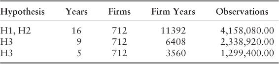
This study seeks to evaluate, in a global context, the impact of the Sarbanes-Oxley Act on a particular risk measure of importance to investors (risk-adjusted returns), and two measures of risk due to asymmetry (upside and downside risk). A unique dataset permits a dual evaluation of the law's impact upon such measures in leading non-U.S. economies as well (i.e., “ripple effects”). Hypotheses are empirically evaluated on a sample (n = 712) of the largest U.S. and European firms (control) using daily return data from 1993 through 2009—one of the most extensive data sets employed in the literature on this topic to date. The reliability of our risk measures is carefully evaluated using multiple approaches, including Fama-MacBeth regressions. We then employ a series of difference-in-differences analyses to empirically assess Sarbanes-Oxley's impact upon equity risk.

The findings suggest Sarbanes-Oxley decreased both risk-adjusted returns and upside risk, whereas downside risk fails to explain the cross section of returns for the largest U.S. firms. From a global perspective, we suggest that the enactment of Sarbanes-Oxley's in the United States motivated leading non-U.S. economies to adopt similar regulatory measures, which caused “ripple effects”—for example, effects similar to those documented in this paper—in leading non-U.S. economies.

The findings suggest that comprehensive financial regulations, such as the Sarbanes-Oxley Act, are properly envisaged at the global level, as their impact is not confined to the home country. In an increasingly globalized economy, investor welfare is likely to be influenced—directly as well as indirectly—by economic and financial regulation(s) enacted in foreign economies. Arguably, this suggests the pivotal importance of effective mechanisms of global governance, such that a purely domestic approach to regulation may be shortsighted. In either case, the findings of this study are entirely relevant if regulators are to consider the broader, global impact of regulation upon investor welfare.

This is the first study to empirically analyze, within a global framework, Sarbanes-Oxley's risk implications without relying upon a series of simple mean variance analyses. Substantive research documents that the methodological approach we employ is more precise, reliable, as well as “investor relevant.” Furthermore, we seek to assess the law's impact upon leading non-U.S. equity markets, a first for the literature. Consequently, this study provides a robust evaluation of the law's (international) impact upon firm (equity) risk, making an important contribution to the literature.

Introduction

After the collapse of Enron and reports of accounting fraud at WorldCom, HealthSouth, and other leading firms, the U.S. Congress enacted the Sarbanes-Oxley Act of 2002. It is widely considered the most comprehensive economic regulation since the New Deal. However, the precise impact of the law upon firms has been shrouded in controversy. More recently, a growing body of research suggests that, on average, firms and investors are likely to experience negative consequences.¹

A particular area of concern is the law's impact upon corporate risk. Bargeron and colleagues (2010) report a decrease in corporate risk-taking;² Akhigbe and colleagues (2009),³ and Akhigbe and Martin (2006)⁴ suggest an increase immediately following the law's enactment. Related research reports a discriminatory impact upon high-risk and well-governed firms,⁵ an increase in managerial risk aversion,⁶ and a variety of unintended consequences.⁷ These and other studies analyzing Sarbanes-Oxley's impact upon risk rely exclusively upon simple mean variance analyses, and therefore fail to take into account investor preference for loss aversion.⁸

The impact of Sarbanes-Oxley on asymmetric measures of risk has yet to be evaluated within the literature: namely, upside and downside risk.⁹ Furthermore, while research demonstrates a reduction in mean-variances due to Sarbanes-Oxley,¹⁰ of more relevance to investors is its impact upon equity returns per unit of risk. This is the first empirical attempt to analyze, within a global context, Sarbanes-Oxley's impact upon specific measures of risk that are likely to be of greatest concern to investors: upside and downside risk, and firms' ability to generate returns efficiently.

First, however, we rigorously evaluate the ability of our risk measures to explain cross-sectional equity returns independent from the unconditional beta. The result is a robust evaluation of Sarbanes-Oxley's impact upon “investor relevant” risk. We examine three basic research questions: (1) Is upside and downside risk empirically distinct from the unconditional beta?; (2) What is Sarbanes-Oxley's impact upon these risk types for the largest U.S. firms?; and (3) What impact did Sarbanes-Oxley have on leading, non-U.S. equity markets?

Three main findings are suggested: (1) upside risk and risk-adjusted returns represent significant factors that help to explain the cross-section of equity returns, even after controlling for important firm covariates that influence risk; (2) that Sarbanes-Oxley negatively impacted firms' risk-adjusted returns—for example, by reducing their ability to generate returns efficiently—and decreased upside risk; and (3) that the enactment of the law in the United States encouraged the adoption of similar, albeit less stringent laws in leading, non-U.S. economies, as needed to restore some sort of “global regulatory equilibrium.” This produced what we refer to as “ripple effects”—risk effects similar to those documented in this paper, but in leading non-U.S. economies. In analyzing Sarbanes-Oxley's global impact, our study represents an important contribution to the literature.

Extending CAPM

Under the capital asset pricing model (CAPM), (equity) risk is defined in terms of the variability of a firm's stock returns.¹¹ According to CAPM, the appropriate measure of risk of any asset or portfolio p is given by its “beta”:

5.1

where r_p and r_mkt are the random returns on portfolio p and on the market, respectively, and r_f equals the risk free rate of interest. In equilibrium, all assets and portfolios will have the same return after adjustment for risk, implying the following:

5.2

Research to date has sought to evaluate Sarbanes-Oxley's risk impact exclusively through the lens of CAPM—for example, via a series of simple mean-variance analyses. However, as economists have long noted, such reliance produces several crucial limitations.¹² Equity return distributions tend not to be symmetric but exhibit fat tails with more values on the extreme positive versus negative, given they are left censored.¹³ This causes the standard deviation to underestimate the risk of large movements, decreasing its utility as a precise measure of risk.¹⁴

Furthermore, evaluating the law's impact upon standard deviation—to the exclusion of all other risk measures—is to (falsely) assume that investors agree as to the degree of risk contained in every investment. In practice, investors exhibit a diversity of perceptions regarding risk. For instance, institutional investors consider “investment risk” relative to the possibility of underperforming a specific benchmark.¹⁵

Another serious limitation of the CAPM framework is that upside and downside risks are held to be equally distasteful. This is contradicted by a consistent empirical finding that investors prefer positively skewed returns, such that upside risk is less important to investors than downside risk.¹⁶ As a cumulative result of these factors, the empirical research as to Sarbanes-Oxley's mean-variance impact suffers from severe limitations. It represents a natural extension of CAPM to take into account the asymmetric treatment of risk by evaluating asymmetric downside and upside betas.¹⁷ Consequently, this study extends the literature on Sarbanes-Oxley to include a robust empirical analysis of its impact upon alternative risk types within a global context.

Hypotheses

We evaluate three hypotheses—one invoking parametric and two nonparametric measures—as drawn from a review of multiple literatures.

Hypothesis 1: Sarbanes-Oxley Will Reduce Firms' Risk-Adjusted Returns

Vakkur and colleagues (2010)¹⁸ suggest that Sarbanes-Oxley impacts firm risk by influencing managerial decision making. Managers seek not only to maximize expected return—defined as the anticipated level, timing, and duration of cash flows—but also to optimize the firm risk, per unit of return.¹⁹ This implies that investors prefer firms that generate returns efficiently relative to risk.

We expect Sarbanes-Oxley to reduce risk-adjusted returns essentially by preventing managers from optimizing the delicate relationship between risk and return. Current research, for instance, suggests that the law discriminately impacts risky as well as efficiently run firms,²⁰ and that it strongly incentivizes firm behaviors not supported by the profit objective.²¹

This suggests a general reduction in firms' abilities to generate returns efficiently, as compliance with the comprehensive and punitive law forces managers to make decisions forcing suboptimal solutions to strategic problems. The likely result is a deterioration in firms' (equity) risk-return relationship as strategically optimal projects are surrendered to compliance concerns. As a result, risk-adjusted returns can be expected to decline, as firms lose their ability to manage risk efficiently due to the costly law.

Hypothesis 2: Sarbanes-Oxley Will Decrease Firms' Upside Risk

Upside risk refers to the extent to which the value of a security may increase beyond forecasted levels. Prior regulation has been demonstrated to influence upside risk: Simon (1989)²² documents a significant decrease in upside risk due to the 1933 Securities Act, which enhanced disclosure requirements. We hypothesize Sarbanes-Oxley to have a similar impact for several reasons. Small cap firms tend to have especially pronounced upside risk,²³ and the law is widely known to exercise a negative impact upon such firms.

As a result, upside risk for small firms can be expected to decrease, as they are forced to divert scarce resources away from high growth projects. As small firms contribute disproportionately to the upside risk of the overall equity market,²⁴ it follows that the upside risk of the overall U.S. equity market will likely decrease as well.

A second factor suggesting a reduction in upside risk is Sarbanes-Oxley's documented, negative impact upon innovative and efficiently governed firms,²⁵ which also contribute significantly—if not disproportionately—to the upside risk of the U.S. equity market. As a result, Sarbanes-Oxley is again likely to reduce market upside risk.

Since investors are disproportionately concerned with downside risk, a reduction in upside—and not downside—risk may seem less relevant. Nevertheless, upside “risk” represents an important source of investor benefits given the natural desire to earn excess (positive) returns. Consequently, a potential reduction in upside risk attributable to Sarbanes-Oxley is likely to harm investors, reducing any ability to earn excess returns.

Hypothesis 3: Sarbanes-Oxley Will Decrease a Firm's Downside Risk

Downside risk is a relative term—it may be defined as the annualized standard deviation of returns below a specific target.²⁶ Generally speaking it is the risk that an investment will underperform, producing investor losses relative to some predetermined benchmark. That Sarbanes-Oxley exercises an influence upon (mean variance) risk is widely documented within the literature. Furthermore, as argued in Hypothesis 2, it can be reasonably expected to reduce upside (equity) risk. Following the same logic, this hypothesis suggests that Sarbanes-Oxley may exert a relatively marginal effect in reducing downside risk, which investors generally loathe.

As previously suggested, the comprehensive and stringent law can be expected to inspire tepidity in managers, resulting in risk reduction and potentially even firm rigidity.²⁷ However, this same effect may also reduce the frequency of managerial decisions resulting in unanticipated firm losses, given the tremendous duress under which the law forces firms to operate. This suggests that Sarbanes-Oxley may enable firms to be ever more vigilant during periods of market decline, and therefore exercise a deterrent effect, discouraging managers from taking unacceptable risks. To the degree that this is true, Sarbanes-Oxley can be expected to reduce downside volatility—and therefore the likelihood of larger than expected losses—during periods of market decline.

However, this effect is likely to be marginal, especially due to the large firm sample used to test the hypothesis. Such firms—due in part to their overall size and market position—faced tremendous scrutiny prior to Sarbanes-Oxley. Consequently, any effect produced by the law is likely to be incrementally small. Nevertheless, even a relatively small impact may be perceived as significant to investors, given the general aversion to downside risk.²⁸

Evaluation of Risk

To evaluate Hypothesis 1—Sarbanes-Oxley's impact upon firms' risk-adjusted returns—we evaluate the Sharpe ratio, a standard deviation based measure of risk-adjusted returns.²⁹ A strong Sharpe ratio suggests high returns per unit of risk—for example, firms are generating returns efficiently. The Sharpe ratio is calculated by subtracting the return of the 90-day Treasury bill from the periodic return generated by the portfolio of sample firms (e.g., United States, EU), and then dividing by the portfolio standard deviation.

Our evaluation strategy for Hypotheses 2 and 3—the risk implications of Sarbanes-Oxley due to asymmetry—benefits greatly from Ang, Chen, and Xing (2006),³⁰ who demonstrate a practical means of evaluating asymmetric risk measures for a given investor whose aversion to losses far exceeds attraction to gains.

Risk Measures

The CAPM Beta—i.e., β = cov (r_i; r_m)/var(r_m)—does not sufficiently encompass the risk-return relationship of an individual equity.³¹ While expected returns increase with β, this measure fails to capture all relevant risk, given the overriding concern for downside risk (i.e., A < 1). Consequently, our risk evaluation of Sarbanes-Oxley extends the CAPM framework to include empirically validated measures of asymmetric risk.

Following Ang, Chen, and Xing (2006),³² our proxy for upside risk (i.e., β⁺) is equivalent to our downside risk measure, except it is conditioned on market movements with excess return above the market average. Therefore, equation 5.3 is calculated as follows:

5.3

Conversely, a satisfactory measure of downside risk should be able to describe the cross-section of expected returns. Following Bawa and Lindenberg (1977)³³ we adopt the following measure for equation 5.4:

5.4

where r_i (r_m) is security i's (the market's) “excess” return, and u_m is the average market (excess) return. Ang, Chen, and Xing (2006)³⁴ note that the three beta measures (e.g., upside, downside, and CAPM) covary slightly. In order to disentangle their effects we also evaluate the following measures: a “relative upside” beta (i.e., β⁺ − β) as well as the “spread” between upside and downside risk, (β⁺ − β⁻). We also calculate downside beta relative to the regular CAPM beta, or: β⁻ − β. These additional measures test whether our beta for upside and downside risk capture firm-specific information that is distinct both from the CAPM beta as well as from one another.

Data and Empirical Model

The initial sample comprises the 500 largest U.S. firms, as represented by the 2009 S&P 500, and the 500 largest European firms, as listed on the 2009 Bloomberg European 500 Index (BE500). The BE500 includes equities listed on 16 different European exchanges: The London Stock Exchange, Euronext (Paris), and the Xetra (Frankfurt) are the three most frequently represented. This represents arguably the most comprehensive dataset used to analyze the impact of Sarbanes-Oxley.

Large firms are particularly relevant in any study seeking to analyze the impact of comprehensive regulation, given their vast importance to the overall economy. The S&P 500, for instance, comprises nearly 75 percent of all U.S. economic activity—or $3.5 trillion—and the BE500 is similarly representative of the EU. In employing a sample of large firms we also avoid the illiquidity effects attributed to small firms,³⁵ though we increase the difficulty of achieving statistically significant results: Risk due to asymmetries is most prevalent among small firms³⁶ (see Table 5.1).

Table 5.1 Market Capitalization

Market Cap (Adjusted $ Billion)	S&P 500	BE 500
Average	18.64	17.90
Largest	291.75	171.56
Smallest	1.01	0.81

Since Sarbanes-Oxley became law at the end of July 2002, the return data is further divided into firm years, which begin on August 1 and end on July 30. Furthermore, following a difference-in-differences analysis strategy, it is then divided into four observation groups: (1) U.S. risk measures pre-Sarbanes-Oxley, (2) U.S. risk measures post-Sarbanes-Oxley, (3) EU risk measures pre-Sarbanes-Oxley, and (4) EU risk measures post Sarbanes-Oxley.

Unless otherwise noted, we analyze the daily stock market returns from January 1, 1993 through December 31, 2009. We follow a two-pronged empirical approach. First we calculate all risk measures using daily data over shorter samples—versus lower frequency data over extended samples—as this offers greater statistical power. Following Fama and French (2005),³⁷ evaluations focus on a series of short one-year samples using daily data, rather than a single long sample using monthly data.

As an added reliability measure we also calculate each risk measure on a monthly basis, and compare these to our annual estimates. Calculated risk measures are then used to conduct a series of difference-in-differences analyses, in order to evaluate the impact of Sarbanes-Oxley upon “investor-relevant” risk types.

Firms that lack data for more than five periods are dropped from the sample, as are all foreign cross listed firms—producing a final sample of 712 firms. Rather than follow precedent within the empirical finance literature by dropping financial firms—which comprise roughly 25 percent of each index—we retain them. Foerster and Sapp (2005)³⁸ demonstrate that eliminating financial services firms can influence both findings of statistical significance as well as coefficient magnitudes. Consequently, our strategy is mixed: Initial models do not control for financial firms, while follow-up models do (e.g., as a robustness test).

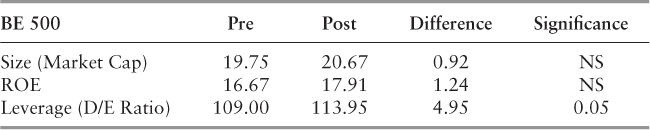
As this is a study of risk, we control for size (market capitalization), leverage (debt:equity ratio) and profitability (ROE)—three factors intricately linked to equity risk,³⁹ as shown in Tables 5.2 and 5.3.

Table 5.2 S&P 500 Data

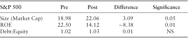
Table 5.3 BE 500 Data

Estimation and Results

To increase the accuracy of our estimates, each risk measure (e.g., Sharpe ratio; CAPM, upside and downside beta) is rigorously evaluated to ensure measure reliability. At the beginning of each one-year period at time t₀, we calculate the following betas for the subsequent 12-month period: CAPM, upside, downside, relative upside, relative downside, and “range” (i.e., upside – downside).

Following Fama and French (1992),⁴⁰ we form equal weighted portfolios based upon various factor loadings, except that portfolios are sorted according to intra-period risk measure(s), which are then used to predict average returns for the same—versus a subsequent—period.⁴¹ Furthermore, portfolios are segmented according to period: pre and post Sarbanes-Oxley. Each portfolio is listed in Table 5.4 according to the average actual return for the same period.⁴²

Table 5.4 Portfolios by Average Actual Return

One advantage of this approach is that it does not require an assumption of constant or time invariant measures of risk, given the wealth of research strongly suggesting risk exposure is time varying (e.g., Fama and French 1997; Lewellen and Nagel 2006).⁴³ A second advantage is that we control for additional firm covariates to increase the precision of our estimates: log-size, leverage, prior 12-month excess return beginning at t₀, and the

standard deviation of firms' excess returns. Additionally, to ensure that outliers are not driving the results, the data is Winsorized.⁴⁴

Our calculated risk measures appear to make sense and to be relatively stable. For instance, as we would expect, a monotonically increasing pattern exists between average returns and CAPM beta. As shown in Panel A, Portfolio_pre-SOX 1(5) has an average excess return of 3.48 percent (14.17 percent) per annum, while Portfolio_post-SOX 1(5) has an annual average excess return of 3.34 percent (13.94 percent). This is consistent with the previous literature that high (CAPM) beta equities, on average, tend to reward investors with superior returns (Black et al. 1972). Furthermore, the results suggest a significant correlation between high average returns and high measures of the three betas: CAPM, upside, and downside.

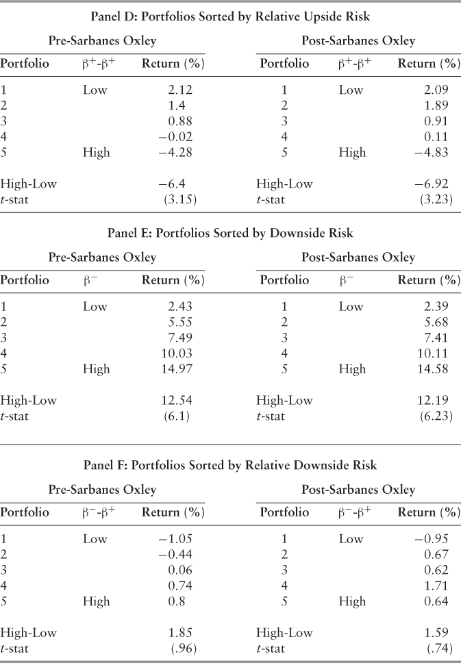
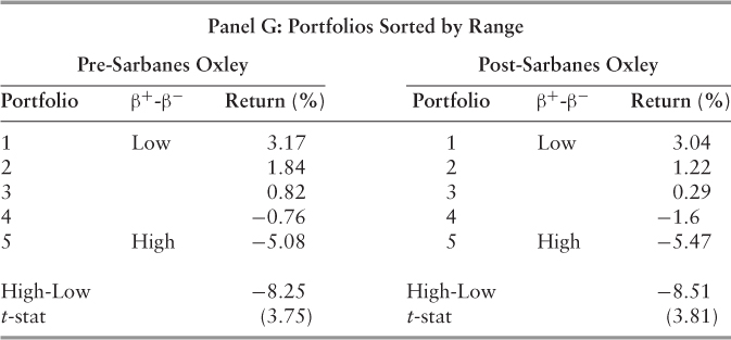
Controlling for the effects of the unconditional beta, the calculated measures for relative upside risk suggest that upside risk is a distinct construct that captures unique firm information. However, the same does not hold true for our measure of relative downside risk, which fails to achieve statistical significance. Contrary to Ang, Chen, and Xing (2006),⁴⁵ we fail to conclude that the downside risk beta captures a distinct measure of firm risk relative to the unconditional beta. Potentially, this may be a statistical artifact of our sample, which contains the largest U.S. (and EU) firms, since small and extremely volatile firms tend to exhibit high measures of downside risk.⁴⁶ Apart from this, our results comport well with prior research, and suggest stable risk measures that capture unique, firm-specific information not contained in the CAPM beta.

Difference-in-Differences Analysis

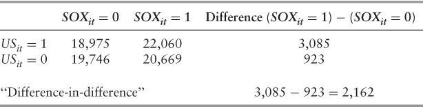
The second step in our methodological approach is to conduct a series of difference-in-differences analyses to estimate Sarbanes-Oxley's impact upon equity risk. Difference-in-differences models measure the difference in outcome over time for the “treatment group” compared to the difference in outcome over time for the control group. As depicted in the following equation 5.5, the difference-in-differences estimator may be expressed as:

5.5

The associated standard error is then measured with the following regression (equation 5.6):

5.6

The term may then be decomposed as follows, to produce equation 5.7:

5.7

Therefore, captures the pre/post change in standard deviation for the sample of foreign-listed firms. For observations falling within the pre-Sarbanes-Oxley time period, SOX_i = 0 and US_i = 1, such that SOX_i * US_i = 0. Consequently, the previous equation may then be decomposed into the following term (eq. 5.8):

5.8

Consequently, measures the mean standard deviation differential between U.S. and EU firms not attributable to Sarbanes-Oxley. refers to the average equity standard deviation for non-U.S. listed sample firms.

For post Sarbanes-Oxley observations of foreign (non-U.S.) listed firms, SOX_i = 1 and US_i = 1, such that SOX_i * US_i = 1. Consequently, equation 5.8 may be decomposed into the following equation 5.9:

5.9

Therefore, measures the change in standard deviation for U.S. firms, which may be attributed to Sarbanes-Oxley (i.e., the difference-in-differences effect). All results are provided in Table 5.5.

Table 5.5 Change in Standard Deviation for U.S. Firms

Fixed Effects Estimation

We now combine all years and run the model across all t (i.e., 1993 to 2009). The fixed effect, α_i accounts for all unobserved firm-specific effects, permitting a more precise estimate of Sarbanes-Oxley's influence upon firm risk. This specification is preferred in that it explains some of the variance that was previously captured in the error term, u_it. Furthermore, failing to model for the fixed effect, α_i, will bias the estimation of the difference-in-differences effect to the degree that the fixed effect is correlated with either US_it or SOX_it.

We use Stata to perform the OLS regression on panel data with fixed effects beginning with Model 3. The difference-in-differences effect is statistically significant for all three risk measures: Sharpe ratio and upside and downside beta, while the coefficient signs are in the hypothesized directions. To further improve the predictive ability of the model, in Model 4 we now add dummy variables for time, one per year.

The model now controls for all of the variables that have a common effect across all firms in a given year. For instance, macro level variables in the U.S. and the EU are typically correlated, such that they exert a common effect upon all firms. The new introduced variable η_t represents a constant common to every firm at time t. The resultant difference-in-differences effect is now statistically significant at the 99 percent level of confidence for the Sharpe ratio and upside beta, while the downside beta achieves statistical significance at the 95 percent confidence level—all three hypotheses receive empirical support as the effect is again in the hypothesized direction.

The relevant coefficients are now slightly larger, in absolute value terms, with the time dummies included in the regression. However, the findings suggest that Sarbanes-Oxley's impact upon downside risk is very small, and therefore likely to be economically insignificant. Furthermore, given that our prior results (see Table 5.4) failed to confirm the independence of our downside risk measure from the unconditional beta, little significance is given to these results.

In the next model, Model 5, we control for observed firm characteristics known to influence risk: size (i.e., stock market capitalization) and leverage (i.e., the debt: equity ratio).⁴⁷ The addition of the control variables to the regression has a noticeable impact: The difference-in-differences effect is now much stronger, regardless of the measure analyzed. In terms of the Sharpe ratio, for instance, the difference-in-differences effect more than doubles when capitalization and leverage are added as control variables, again suggesting that Sarbanes-Oxley reduced firms' risk-adjusted returns.

In order to determine the individual impact of each control variable upon the dependent, we now run the same equation twice, including capitalization (Model 6) and leverage (Model 7) separately. The results suggest that firm size negatively impacts risk-adjusted returns and upside risk, whereas increased leverage appears to have a small but positive effect upon downside risk. According to economic theory, larger firms should have less volatile profits since they are better diversified, have better access to financial markets, and tend not to grow as quickly as small firms. Improved access to financial markets allows firms to hedge risks and smooth profits better than small firms. Relatively slower growth is associated with less variation in growth rates: Since future growth prospects change less rapidly for large firms, their stock prices tend to fluctuate less than for small firms. Since stock price is equivalent to the expected discounted flow of future profits, returns are therefore less volatile.

Table 5.6 shows market capitalization for U.S. and EU firms before and after Sarbanes-Oxley. Market capitalization increases more for U.S. than for EU firms over the period sampled. Failing to include capitalization in the regression would bias the difference-in-differences coefficient downward, since increases in firm capitalization are correlated with reductions in risk-adjusted returns and upside risk.

Table 5.6 Market Capitalization for U.S. and EU Firms

Vakkur and Herrera (2011)⁴⁸ suggest that Sarbanes-Oxley's mean-variance reducing impact may be positively correlated to firm size for those firms in the upper tail of the size distribution. Consequently, in Model's 8 and 9 we extend an evaluation of their working hypothesis to our sample and measures of risk. Results suggest that Sarbanes-Oxley's negative impact upon risk-adjusted returns and upside risk is indeed greatest for the largest firms in our sample.

Model's 10 and 11 seek to provide an additional test that Sarbanes-Oxley—and not something else—is actually driving the results. In Model 10, for instance, the base year is 1996: The “pre” period is all data prior to 1996, while the “post” period is composed of all data including the base year and beyond. In Model 11, we adopt the same technique, except that the base year is now 1999. A statistically significant finding in years other than the policy intervention would require further analysis. Both models fail to achieve statistical significance (α = .05) for either risk measure.

Perhaps more relevantly, the sign on the difference-in-differences coefficient is, in each case, positive—opposite of what we find in evaluating Sarbanes-Oxley. Consequently, our main findings are that Sarbanes-Oxley reduced firms' risk-adjusted returns and upside risk do not appear to be a statistical artifact, the result of pure chance.

Robustness Tests

We now seek to demonstrate that study results are not statistical artifacts, nor are they dependent upon the way we have measured asymmetries in betas or the design of our empirical tests. For instance, we test whether our risk estimates are unduly influenced by the choice of cutoff date. Our upside and downside risk measures use returns relative to average market excess return. However, average market returns vary across time and may contain peaks and troughs in the data. Therefore, instead of relying upon the average market excess return as the point of distinction between up and down-markets, the risk-free rate may also be employed.⁴⁹ Consequently, we recalculate downside and upside beta relative to this alternative cutoff points as follows:

Table 5.6 reports the time series averages of the cross-sectional correlations of CAPM beta and the various downside and upside risk measures. For instance, the CAPM beta is significantly correlated with our downside (.94) and upside beta (.77) measures. However, the correlation between downside and upside beta—.56—is not statistically significant, suggesting they capture distinct firm-specific information. Both the upside (downside) beta and the risk-free upside (downside) beta are strongly correlated (.98 for each) with one another.⁵⁰

This provides further evidence that our calculated measures for risk due to asymmetry are relatively stable and consistent. The correlation between CAPM and upside beta (.76) also suggests that the two measures capture distinct firm-specific information. However, the strong correlation between CAPM and downside beta (.94) suggests that the latter fails to provide a distinct measure of risk for our sample.

Our second robustness test is to include a control for financial services firms. It is common practice for empirical researchers to exclude financial services firms from their sample data altogether, as relatively high leverage ratios produce an increased sensitivity to financial risks.⁵¹ In both Models 12 and 13 (see Table 5.6), the indicator variable modeling financial services firms is highly significant. For instance, the results from Model 12 suggest that financial services firms, between 1993 and 2009, measured slightly higher than other firm types in terms of risk-adjusted returns and upside risk. Modeling for this effect reduces the bias in our (difference-in-differences) estimates of the true coefficients.

As a final test, we employ cross-sectional Fama-MacBeth regressions to demonstrate that our risk measures capture distinct firm-specific information relative to various firm characteristics noted in the literature. We regress firm returns over a continuous 12-month time period on the unconditional, downside, and upside beta, as well as upon the Sharpe ratio, all from the same period. Excess returns are analyzed as based upon the equivalent 12-month period that is used to calculate each measure of risk.

Due to the annual timeframe with overlapping monthly frequencies, we estimate coefficient standard errors using 12 Newey-West (1987a) lags. Regression results are contained in Table 5.6. We control for the following firm covariates all measured in the same 12-month time period: size-logged, leverage, the prior 12-month excess returns of the firm beginning at t₀, and standard deviation of excess returns. All independent variables are Winsorized at the 1 percent and 99 percent levels to ensure that outliers are not unduly influencing the results.

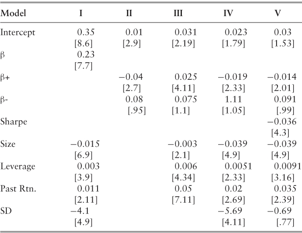
Regression I of Table 5.6 depicts a familiar pattern of cross-sectional returns: Smaller firms tend to have high average returns, while leveraged firms and those with strong positive returns in prior periods tend to exhibit high returns in the current period as well. Results also suggest low average returns for firms with very volatile returns.⁵² In Regressions II–V, we evaluate the upside and downside beta, as well as the Sharpe ratio, a proxy for risk-adjusted returns. Regression II, which contains no control variables, suggests a discount for equities with high upside risk, while the downside risk beta is statistically insignificant, confirming our earlier analyses (see Table 5.4). Regression III shows that any reward for upside risk is robust to controls for size, leverage, and momentum effects, while downside risk is again insignificant. Furthermore, inclusion of the asymmetric beta risk measures fails to remove the size, leverage, or momentum effects, although the associated coefficients do change.

Regression IV includes a control for standard deviation, which reduces the absolute value of the upside risk coefficient without affecting its statistical significance. Our risk evaluation framework—drawn largely from Gul (1991)⁵³—assumes that investors are preoccupied with downside risk, and implies a discount for upside risk. Since the downside risk beta is statistically insignificant in all five models, we fail to observe this specific pattern, though results do suggest a discount for upside risk. Contrary to Ang, Chen, and Xing (2006),⁵⁴ our results suggest that it is upside rather than downside risk that dominates in the cross-section, at least for the largest U.S. firms.

In Regression V, our measure for risk-adjusted returns is added to the regression model and proves highly significant. The coefficient suggests a premium for equities offering relatively high risk-adjusted returns, consistent with economic theory. Furthermore, the addition of the Sharpe ratio drives out any effect for standard deviation, which is no longer statistically significant as might be expected. Most relevant is that upside risk retains its significance, although both the coefficient and the associated t-stat are now smaller.

The results of our Fama-MacBeth regressions support the results of our prior analyses: Upside risk (discount) and risk-adjusted returns (premium) appear to be stable and dominant characteristics of the largest U.S. firms in the cross section. As a result, a rigorous statistical analysis of Sarbanes-Oxley's impact upon these large firm risk factors—as we present in this paper—provides a meaningful evaluation of the law. Overall, our robustness analyses suggest that our main study findings are consistent and reliable.

Discussion

Panel regressions employing fixed effects and time dummies produced a difference-in-differences effect significant at the 99 percent confidence level for both the Sharpe ratio and our upside risk beta. Both Hypothesis 1—Sarbanes-Oxley reduces firms' risk-adjusted returns and Hypothesis 2—upside risk—appear to receive strong support. In terms of Hypothesis 3—upside risk—separate analyses failed to confirm that our downside risk beta captures distinct firm-specific information relative to the unconditional beta for the largest U.S. firms.

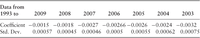
Arguably, Sarbanes-Oxley's impact was most pronounced immediately after it was implemented in 2002, and then decreased gradually over time. We provide a generic test for this hypothesis by evaluating the law's effect upon equity volatility over different estimation periods. For instance, running the model over the entire period (i.e., 1993 to 2009) captures the average effect over the period 2002 to 2009. If Sarbanes-Oxley's impact upon various measures of risk is reduced over time, then the difference-in-differences effect can be expected to grow larger as the time period employed is shortened (e.g., 1993–2008 versus 1993–2009). The results of this test, as demonstrated in Table 5.7, seem to suggest that Sarbanes-Oxley's effect on firm risk gradually decreases over time, from the date of implementation.

Table 5.7 Difference-in-Differences Effect Results

One disadvantage of our methodology is the assumption that there were no confounding events—beyond Sarbanes-Oxley—that may have caused the European and U.S. equity markets to differ during the period analyzed. Through 2005, the major European markets became increasingly integrated with the international (U.S.) equity markets. Since that time, European equities—like those in the United States—have been extremely volatile: After reaching all-time highs in 2007, they slumped to their lowest level since the 1930s in 2008. A tepid rally ensued in 2009. During this period, the historically strong and positive correlation between EU and U.S. equity market returns began to unravel somewhat gradually due to several factors.

Whereas the U.S. equity markets responded relatively well to U.S. economic troubles, the EU has struggled to overcome the first major economic crisis since its inception in 1999. A looming financial crisis hit Spain especially hard from 2008 to 2009, as the nation's economy contracted 4 percent, and unemployment levels reached nearly 14 percent. More recently, mounting fiscal crises among Eurozone nations Greece, Ireland, and Portugal as well as nonmember nations Iceland, Hungary, and Romania have created substantive alarm across European financial markets, including even Germany (Hester, 2010).

It may be argued that our study results, as based upon empirical data from 1993 to 2009, may be influenced by these (potentially confounding) effects. Empirical analyses, however, fail to support this interpretation. Results obtained using data over a relatively constrained time period—for example, just two years pre/post Sarbanes-Oxley—indicate that it is the advent of Sarbanes-Oxley—and not European fiscal woes that came several years later—that is driving results.

Further supporting our hypotheses, the effects attributed to Sarbanes-Oxley over this more limited time period are much more pronounced than they are in later years. This seems to suggest an independent effect for Sarbanes-Oxley, and to support the view that study results are not the result of specious correlations.

Global Regulatory Development (i.e., Ripple Effects)

As EU nations gradually responded to Sarbanes-Oxley by adopting regulations mimicking the law, the “differential” impact of Sarbanes-Oxley decreases, as the results suggest. In another words, Sarbanes-Oxley's relative impact decreases over time as leading foreign economies adopt regulations similar to Sarbanes-Oxley, producing what we term “ripple effects.” For instance, the 8th European Union Company Law Directive on Statutory Audit became law in June of 2006 (FERMA/ECIIA, 2010).

As with Sarbanes-Oxley, EU public firms are required to adopt a comprehensive system of internal controls and risk management practices. Consequently, the introduction of comprehensive accounting reform in the U.S. appears—irrespective of its merits, whether pro or con—to have produced ripple effects, as other nations have been led to adopt similar changes, producing effects in their own economies similar to those documented in this paper. The net result is that Sarbanes-Oxley's impact appears less noticeable over time—in relative terms—while in absolute terms it may have changed very little.

Several factors have helped to produce such changes in the global regulatory landscape. Due to a tightly linked, global economy, the introduction of comprehensive regulatory changes by the U.S. can be said to produce “regulatory disequilibrium”—an awkward period in which leading international firms grope for a newfound state of certainty. Europeans, for instance, sarcastically referred to the sweeping changes introduced by “two U.S. Congressman” as having “forced half a million accountants in Europe” to start dancing.⁵⁵

Whereas regulatory compliance among U.S. publicly owned firms was compelled by the stringent law, producing relatively rapid adoption, foreign firms likely faced enormous social and institutional pressures to “keep up” with regulatory “innovations,” especially those promising enhanced protection for investors. Furthermore, Sarbanes-Oxley introduced an awkward and painful state of uncertainty, both for U.S.-listed firms—who were unsure precisely how to comply with the law—and for foreign firms—who were even less clear as to how the law might affect them.

As a result, both U.S. as well as foreign (i.e., non-U.S. listed) firms invested weighty resources in order to grasp, over a period of several years, the full legal, strategic, as well as practical implications of the sweeping new law. Over time, leading economies effected laws that—at least in appearance—mimicked Sarbanes-Oxley. This dramatically reduced uncertainty as well as the social and financial costs of transacting business globally, restoring global “equilibrium” as it relates to regulation.

This lagged effect is consistent with the empirical results: The magnitude of Sarbanes-Oxley's impact upon U.S. equity markets—in relative terms—decreases over time as other nations enact similar changes over a period of years. While the absolute impact of the law may also lessen over time—for example, as firms develop successful adaptations and so forth—the results of this study neither confirm nor refute such an interpretation. It is important to note, however, that the effects we document persist through 2009—the final year of data for this study. This is likely because the EU enacted laws in response to Sarbanes-Oxley that were considerably less stringent, suggesting that quite possibly the Europeans gained critical insights from U.S. experience. EU laws in this regard, for instance, tend to rely more upon principles than rules.

In either case, the study suggests three main findings: (1) upside risk and risk-adjusted returns represent significant factors that help to explain the cross-section of equity returns for the largest U.S. firms, even after controlling for important firm covariates that influence risk, (2) Sarbanes-Oxley negatively impacted firms' risk-adjusted returns—for example, by reducing their ability to generate returns efficiently—and decreased upside risk, and (3) that Sarbanes-Oxley introduced a state of global uncertainty, which—in this example—motivated foreign economies to adopt similar laws. While this helped to restore “global regulatory equilibrium,” it produced “ripple effects”—meaning that effects similar to those documented in this paper were reproduced in foreign economies, a potentially important concern for global investors. This is the first study to make these implications, and therefore it provides an important contribution to the literature.

Table 5.8 closely follows Ang, Chen, and Xing (2006), who list the equal-weighted average returns and risk characteristics of equities sorted according to factor loadings. For each month, we calculate CAPM beta, downside risk, and upside risk using daily continuously compounded returns over the following 12-month period for our sample of S&P 500 firms. For each risk measure, equities are sorted into portfolios (1–5) that form equal-weighted portfolios at the start of each 12-month term. The number of equities per portfolio varies over time. The “Return” column provides the average return in excess of the one-month T-bill rate over the following 12-month period—the equivalent period used to compute the three beta measures. “High-Low” reports the return differential between portfolios 5 and 1; t-stats are calculated using Newey-West (1987) heteroskedastic-robust standard errors with 12 lags. Columns labeled according to CAPM, upside and downside beta report the time-series and cross-sectional average of equal-weighted individual equity betas over the annual holding period. The sample period is from January 1, 1993, through December 31, 2009. Since Sarbanes-Oxley became law at the end of July 2002, the return data is further divided into firm years, which begin on August 1 and end on July 30.

Table 5.8 U.S. Equity Returns Sorted by Calculated Risk Measure

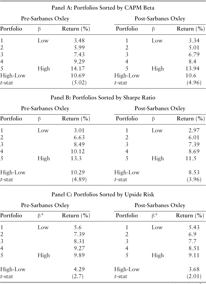
(The pre-Sarbanes-Oxley period ends July 30, 2002, and the post period begins August 1, 2002, and all observations occur at a monthly frequency).

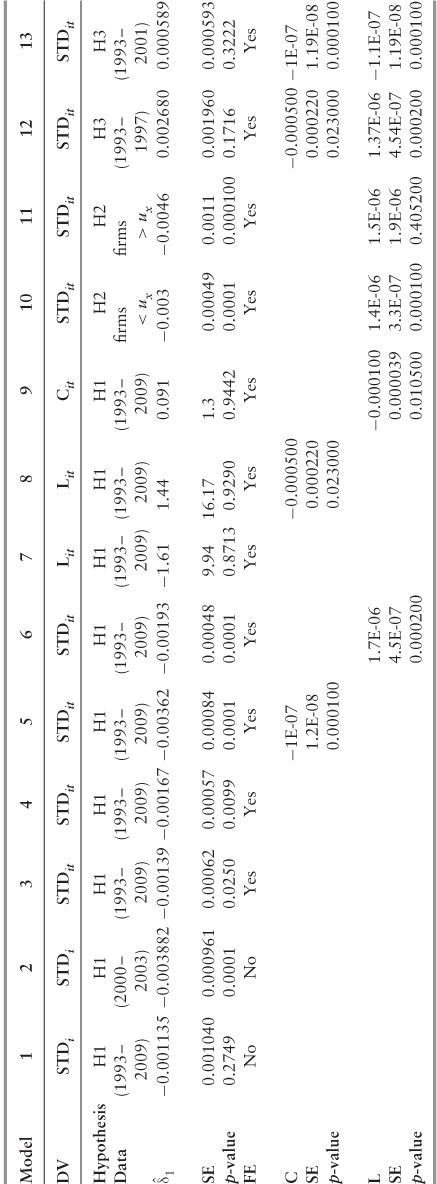
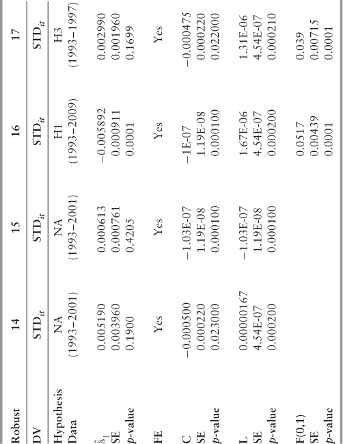
Table 5.9 demonstrates the results of our difference-in-differences analysis with alternate specifications to control for firm size (C), leverage (L), fixed effects (FE) and financial services firms (F). The daily return data covers January 1, 1993 through December 31, 2009, and includes a total of 712 firms from the S&P 500 and the BE 500. Since Sarbanes-Oxley became law at the end of July 2002, the daily return data is further divided into

Table 5.9 Difference-in-Differences Analysis

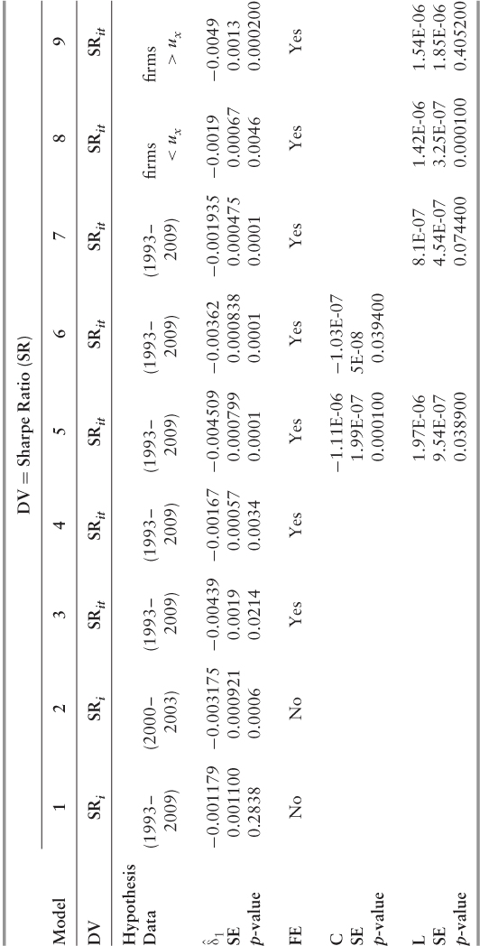
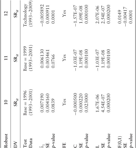
firm years, which begin on August 1 and end on July 30. (The pre-Sarbanes-Oxley period ends July 30, 2002, and the post period begins August 1, 2002, and all observations occur at a monthly frequency—136,704 firm months in the full sample. We report p-values as a test for statistical significance. Results are provided according to the dependent variable—(a) Sharpe ratio (risk-adjusted returns) and (b) upside risk beta.

Table 5.10 lists the time-series averages of cross-sectional correlations for our primary beta measures: CAPM, upside, upside risk-free, downside, and downside risk-free. Both CAPM and upside beta are computed relative to the sample mean market return. All betas are computed based upon daily return from the previous 12-month period. The daily return data covers January 1, 1993 through December 31, 2009 and includes a total of 712 firms from the S&P 500 and the BE500. All observations occur at a monthly frequency—136,704 firm months in the full sample.

Table 5.10 Correlations between Beta Measures

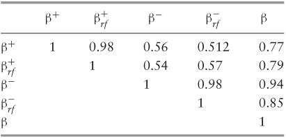
Table 5.11 contains the results of Fama-MacBeth (1973) regressions of 12-month excess returns on firm covariates and calculated risk measures. Daily return data covers January 1, 1993 through December 31, 2009 and includes a total of 712 firms from the S&P 500 and the BE 500. All observations occur at a monthly frequency—136,704 firm months in the full sample. All t-statistics—as listed in brackets—are calculated using Newey-West (1987) heteroskedastic-robust standard errors with 12 lags.

Table 5.11 Fama-MacBeth Regressions

 

 

 

Notes

¹ N. Vakkur, R. P. McAfee, and F. Kipperman, “The Unanticipated Costs of the Sarbanes-Oxley Act of 2002,” Research on Accounting Regulation, 2010; E. Engel, R. M. Hayes, and X. Wang, “The Sarbanes-Oxley Act and Firms' Going Private Decisions,” Journal of Accounting and Economics 44 (2008), 116–145; I. X. Zhang,“Economic Consequences of the Sarbanes-Oxley Act of 2002,” Journal of Accounting and Economics, 44 (2007), 74–115; V. Chhaochharia and Y. Grinstein, “Corporate Governance and Firm Value: The Impact of the 2002 Governance Rules.” Journal of Finance 62 (2007), 1781825.

² L. L. Bargeron, K. M. Lehn, and C. J. Zutter, “Sarbanes-Oxley and Corporate Risk-Taking,” Journal of Accounting and Economics 49 (2010), 34–52.

³ A. Akhigbe, A. D. Martin, and T. Nishikawa, “Changes in Risk of Foreign Firms Listed in the U.S. Following Sarbanes-Oxley.” Journal of Multinational Financial Management 19 (2009): 193–205.

⁴ A. Akhigbe and A. D. Martin, “Valuation Impact of Sarbanes-Oxley: Evidence from Disclosure and Governance within the Financial Services Industry,” Journal of Banking and Finance 30 (2006): 989–1006.

⁵ K. Litvak, “Defensive Management: Does the Sarbanes-Oxley Act Discourage Corporate Risk-Taking?” 3rd Annual Conference on Empirical Legal Studies Papers, SSRN, 2008. http://ssrn.com/abstract=1120971.

⁶ D. A. Cohen, A. Dey, and T. Z. Lys, “The Sarbanes-Oxley Act of 2002: Implications for Compensation Contracts and Managerial Risk-Taking.” SSRN Working Paper, 2007.

⁷ N. Vakkur, R. P. McAfee, and F. Kipperman, “The Unanticipated Costs of the Sarbanes-Oxley Act of 2002.” Research on Accounting Regulation, 2010.

⁸ D. Kahneman and A. Tversky, “Prospect Theory: An Analysis of Decision under Risk,” Econometrica 47, no. 2 (1979): 263–91.

⁹ By definition, upside (downside) risk is that portion of a firm's (observed) equity variance that can be explained by equity market movements during periods of stock market increases (trades lower).

¹⁰ N. Vakkur and Z. J. Herrera, “The PSLRA, Sarbanes-Oxley and Large Firm Risk.” Working Paper, Trident University, Cypress, CA, 2011.

¹¹ H. M. Markowitz, “The Early History of Portfolio Theory: 1600–1960,” Financial Analysts Journal, 55, no. 4 (2011): 5–16; W. F. Sharpe, “Capital Asset Prices: A Theory of Market Equilibrium under Conditions of Risk,” Journal of Finance 19, no. 3 (1964): 425–442.

¹² F. Sortino and R. Vandermeter, “Downside Risk.” Journal of Portfolio Management 17 (1991): 27–32.

¹³ Sharpe, “Capital Asset Prices”; S. A. Ross, “The Arbitrage Theory of Capital Asset Pricing,” Journal of Economic Theory, 13, no. 3 (1976): 341–360; R. Bookstaber and R. Clarke, “Problems in Evaluating the Performance of Portfolios with Options,” Financial Analysts Journal 41 (1985): 48–62.

¹⁴ B. Mandelbrot and R. L. Hudson, The (Mis)behavior of Markets: A Fractal View of Risk, Ruin, and Reward (New York: Basic Books, 2004).

¹⁵ N. Riddles, “A Portfolio Manager's View of Downside Risk.” In Managing Downside Risk in Financial Markets: Theory, Practice, and Implementation, F. A. Sortino and S. E. Satchell, eds. (New York: Elsevier, 2001).

¹⁶ A. Kraus and R. Litzenberger, “Skewness Preference and the Valuation of Risk Assets.” Journal of Finance, 1976, 31, 1085–1100; M. Grinblatt and S. Titman, “Portfolio Performance Evaluation: Old Issues and New Insights.” Review of Financial Studies 1989, 2, 393–421; P. Dybvig and J. Ingersoll, “Mean Variance Theory in Complete Markets.” Journal of Business, 1982, 55, 233–252.

¹⁷ V. S. Bawa and E. B. Lindenberg, “Capital Market Equilibrium in a Mean-Lower Partial Moment Framework,” Journal of Financial Economics 5 (1977): 189–200.

¹⁸ Vakkur, McAfee, and Kipperman (2010).

¹⁹ E. F. Fama and K. R. French, “Common Risk Factors in the Returns on Stocks and Bonds,” Journal of Financial Economics 33, no. 1 (1993): 3–56.

²⁰ Litvak, “Defensive Management.”

²¹ Vakkur, McAfee, and Kipperman (2010).

²² C. J. Simon, “The Effect of the 1933 Securities Act on Investor Information and the Performance of New Issues,” American Economic Review 79 (1989): 295–318.

²³ E. F. Fama and K. R. French, “The Cross-Section of Expected Returns,” Journal of Finance 47 (1992): 427–466.

²⁴ Ibid.

²⁵ Litvak, “Defensive Management.”

²⁶ A. J. Ang, J. Chen, and Y. Xing, “Downside Risk,” Review of Financial Studies 19, no. 4 (2006): 1191–1239.

²⁷ Litvak, “Defensive Management”; D. A. Cohen, A. Dey, and T. Z. Lys, “The Sarbanes-Oxley Act of 2002: Implications for Compensation Contracts and Managerial Risk-Taking,” SSRN Working Paper; N. Vakkur, R. P. McAfee, and F. Kipperman, “The Unanticipated Costs of the Sarbanes-Oxley Act of 2002.” Research on Accounting Regulation, 2010.

²⁸ A. Kraus and R. Litzenberger, “Skewness Preference and the Valuation of Risk Assets,” Journal of Finance 31 (1976): 1085–1100; Kahneman and Tversky, “Prospect Theory: An Analysis of Decision under Risk.”

²⁹ An alternative would be to use alpha. However, alpha retains meaning only when the R2 is particularly high (> .75). Additionally, the Sharpe ratio measures return volatility in absolute terms, versus relative to an index.

³⁰ Ang et al., “Downside Risk.”

³¹ Ibid.

³² Ibid.

³³ V. S. Bawa, and E. B. Lindenberg, “Capital Market Equilibrium in a Mean-Lower Partial Moment Framework,” Journal of Financial Economics, 5 (1977): 189– 200.

³⁴ Ang et al., “Downside Risk.”

³⁵ Ibid.

³⁶ C. R. Harvey and A. Siddique, “Autoregressive Conditional Skewness,” Journal of Financial and Quantitative Analysis 34, no. 4 (1999): 465–477.

³⁷ E. F. Fama and K. R. French, “The Value Premium and the CAPM.” Working Paper, Dartmouth University, 2005.

³⁸ S. R. Foerster and S. Sapp, “The Dividend Discount Model in the Long-Run: A Clinical Study,” Journal of Applied Finance, 15, no. 2 (Fall/Winter, 2005).

³⁹ J. L. Coles, U. Loewenstein, and J. Suay, “On Equilibrium Pricing under Parameter Uncertainty,” Journal of Financial and Quantitative Analysis 30 (1995): 347–364; M. A. Ferreira and P. A. Laux, “Corporate Governance, Idiosyncratic Risk, and Information Flow,” Journal of Finance 62, no. 2 (2007): 951–990; D. J. Kisgen, “Credit Ratings and Capital Structure,” The Journal of Finance, 2006, 61; ROE was dropped from the model due to collinearity issues.

⁴⁰ E. F. Fama, and K. R. French, “The Cross-Section of Expected Returns,” Journal of Finance 47 (1992): 427–466.

⁴¹ Analyses using value-weighted portfolios produced nearly identical results.

⁴² An analysis of the beta-return relationship for all three risk measures over a 60-month period using monthly returns suggests the same general pattern.

⁴³ E. F. Fama and K. R. French, “Industry Costs of Equity,” Journal of Financial Economics 43 (1997): 153–193; J. Lewellen and S. Nagel, “The Conditional CAPM Does Not Explain Asset-Pricing Anomalies,” Journal of Financial Economics 82, no. 2 (2006): 289–314.

⁴⁴ P. J. Knez and M. J. Ready, “On the Robustness of Size and Book-to-Market in Cross-Sectional Regressions,” Journal of Finance 52, no. 4 (1997): 1355–1382; Any observation above (below) the 99th (1st) percentile is replaced with the corresponding data point at the 99th (1st) percentile.

⁴⁵ Ang et al., “Downside Risk.”

⁴⁶ Ibid.

⁴⁷ ROE was dropped due to an endogeneity problem: As firms' returns increase, so too does volatility.

⁴⁸ N. Vakkur and Z. J. Herrera, “The PSLRA, Sarbanes-Oxley and Large Firm Risk,” Working Paper, Trident University, Cypress, CA, 2011.

⁴⁹ Ang et al., “Downside Risk.”

⁵⁰ Reproducing both Tables 5.1 and 5.2 using the alternative, risk-free cutoff point produces virtually identical results.

⁵¹ S. R. Foerster and S. Sapp, “The Dividend Discount Model in the Long-Run: A Clinical Study,” Journal of Applied Finance, 15, no. 2 (Fall/Winter, 2005).

⁵² Ang et al., “Downside Risk.”

⁵³ F. Gul, “A Theory of Disappointment Aversion,” Econometrica, 1991, 59, no. 3 (1991): 667–686.

⁵⁴ Ang et al., “Downside Risk.”

⁵⁵ K. C. Engelen, “How European Regulators Are Handling the Spillover Effects of Sarbanes-Oxley,” The International Economy, 2004, www.international-economy.com/TIE_SU04_Engln.pdf.

 

^a This study appeared in Research in Accounting and Finance under the title: “Ripple Effects: Sarbanes-Oxley's Impact upon Investor Risk in a Global Economy,” by Nicholas V. Vakkur and Zulma Herrera-Vakkur.