
Chapter 12
Multiples: An Overview
12.1 PRELIMINARY REMARKS
12.1.1 Multiples and Discounted Cash Flow
The multiples method enables us to define the equity and/or enterprise value of a company using negotiated prices of stocks of similar firms.
The multiples method seeks to develop a relationship between the actual price of shares of comparable listed companies and an accounting metric (such as net income, cash flows, revenues, etc.). This relationship, that is, the multiple, is then applied to the firm's internal metric in order to determine the value of the company through a simple multiplication.
A valuation performed with multiples is based on two assumptions:
- The company's value changes proportionally to the internal variables chosen as a measure of performance;
- The growth rates of both cash flows and the risk level are constant.
If both these hypotheses are verified, the multiples method gives a more “neutral” measure than the one based on the firm's cash flow (DCF), as it takes into account the market expectations on both the growth rate and the discount rate.
In reality, companies rarely satisfy these two hypotheses: cash flows might have different growth rates and the risk level could vary. Moreover, the best measure of performance to be used to compare different companies is not easily identifiable.
On the other hand, financial methods are usually based on expected cash flows, which relate directly to the company being evaluated, and on the discount rate derived from the risk of the business and of the sector it belongs to. This method, in order to be successful, depends on an accurate estimation of cash flows and of the risk measure as well as on reliable hypotheses assumed to calculate the cost of capital.1
To summarize:
- The financial method requires assumptions on future results and the translation of these hypotheses into cash flow projections. It requires the analysis of the company's risk profile and the consequent estimation of the opportunity cost of capital.
- The multiples method avoids these estimations and takes the expected growth rate and risk appreciation directly from market data through the use of multiples.
Nevertheless, the issue concerning the presence of subjectivity in the estimation process is not completely solved. The valuator selects the group of companies which are most similar to the one under consideration. The extent of comparability across companies is always limited for several reasons: the type of activity performed by the company, its size, its risk profile, and its different leverage ratios.
An Obvious Problem
The previous considerations involve an obvious problem: the core of the multiples method lies in entrusting the market with the correct estimation of growth prospects and risk profiles. Nevertheless, limited comparability across businesses requires some verification of their similarity with the business being evaluated. Such verification assumes that the person calculating these estimates has formed their own judgment about the business prospects. It is easy to fall into a paradox: if the one carrying out the estimation adjusts multiples according to their own expectations, the market approach will inevitably tend to replicate the results obtained with a subjective valuation, leading to a useless duplication.
This obstacle can be easily overcome by analyzing the differences among multiples of the chosen comparable companies based on objective elements. This step is always recommended except in cases when the market approach displays an ideal situation of comparability across businesses, such as industries characterized by uniform technologies, non-substitutable products/services, and similar growth prospects.
12.1.2 Stock Market and Deal Multiples
Multiples can refer to values taken from two different market contexts:
- The stock market
- The market for corporate control
In the former case, they are called stock market multiples. In the latter one, they refer to transactions carried out by comparable businesses and they are called deal multiples.
These two types of multiples usually lead to the estimation of different values. In normal situations, that is, when we face neither speculative phenomena nor a transfer of control, stock multiples express stand-alone values, whereas deal multiples refer to expected market prices.
Therefore, stock multiples cannot provide sufficient information to estimate the market price attached to the entire firm, whereas deal multiples cannot provide reliable stand-alone values.
Analysts usually try to overcome the problem of expected market prices through the adjustment of the valuation estimate obtained through stock market multiples with the so-called acquisition premium in the following way.
As already observed, the procedure associated to this adjustment is quite easy (see Exhibit 12.1). The negotiated price in the case of an acquisition is usually higher than the stock market price because acquisition prices incorporate benefits that buyers expect. On the other hand, in a normal situation, stock prices should mirror stand-alone values.
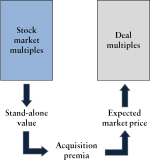
Exhibit 12.1 Stock market and deal multiples
The previous concerns and issues linked to the estimation of the acquisition price will be further discussed in Chapters 14 and 15.
12.1.3 Financial and Business Multiples
Another important distinction is between financial multiples and business multiples. In the former case, multiples seek to identify the connection between a company's equity market price and some important measures such as cash flows, net income, or EBITDA. In the latter case, the company's equity market price is linked to specific elements which are relevant for the business model typical of the sector the company is in. Exhibit 12.2 reports examples of business multiples according to some sectorial grouping of businesses.
Exhibit 12.2 Examples of business multiples
| Utilities Gas distribution
Electricity generation
|
Publishing (newspapers)
|
Internet (web portals)
|
Rental companies
|
Oil companies
|
Financial multiples can be easily interpreted using simple economic rules that enable us to identify their dimension in terms of returns, growth, and risk expectations.
Business multiples, on the other hand, give us a picture of the performance or the position of the company within a specific group with respect to specific drivers.
Therefore, the rationality of business multiples is conditioned on the fact that the identified value drivers for a specific business model effectively capture the sources of value generation for a certain company or industry.
12.2 THEORY OF MULTIPLES: BASIC ELEMENTS
To better understand the topic that will be discussed in this paragraph and to underline the limitations of its assumptions, it is necessary to specify that:
- The discussions reported here will only refer to financial multiples.
- The analysis of multiples is based on the equations discussed in Chapter 7 while addressing analytical methods. As we will see, the choice of a particular type of multiple (P/E, EV/EBIT, and so on) changes the perspective taken by the valuator and the analysis that has to be performed while the factors responsible for the generation of value remain the same.
- Growth, which is the most important element for a good understanding of multiples, is assumed to happen at a rate consistent with a steady growth model.
Several assumptions will therefore be made. Among these, two are the most relevant:
- The return on a new investment opportunity does not change over time.
- The growth rate is constant and is equal to the yield achieved through the systematic reinvestment of a part of the cash flow generated by the company.
12.2.1 Different Types of Multiples
Exhibit 12.3 shows the multiples that are normally used in the valuation of nonfinancial companies. Only some of those multiples—namely the equity-side ones—can be applied to banks and other financial companies as well.2
Two types of multiples can be identified in Exhibit 12.3: multiples calculated only with respect to the market value of equity (P) and multiples calculated with respect to the total value of the company (EV—enterprise value). In this latter case, the numerator of the formula consists of the sum of the value of equity and of net financial debt (to be precise, the market value of debt should be used).
Multiples of the former type allow us to reach an estimate of the value of equity in a direct way. On the other hand, the use of multiples linked to the whole enterprise value leads to an indirect estimation of the value of equity by subtracting the market value of financial debt from the company value.
Exhibit 12.3 The most frequently used multiples and their formulas
| Enterprise value | Equity value |
|
|
|
|
|
|

Exhibit 12.4 shows the relationship between the different balance sheet sections and the multiples which refer to them.

Exhibit 12.4 Balance sheet expressed in market values and its corresponding multiples
In Exhibit 12.5, multiples are divided into two sections: “direct” multiples and “indirect” multiples.
While direct multiples form the relationship between either P or EV and quantities representing economic results, indirect multiples express the relationship between P or EV and quantities which do not directly express how much value the company is able to generate. The book value of equity (BV) or sales actually generate value only if the firm reaches adequate levels of return. If there are differences between the returns of comparable firms and the returns of the firm under consideration, indirect multiples can only be used after making adjustments to take into account the observed differences in terms of returns.
Exhibit 12.5 Direct and indirect multiples
| Direct Multiples | Indirect Multiples |
| P/E (Price/Earnings ratio) | P/BV (Price/Book value) |
| EV/EBIT (Enterprise value/Earnings before interest and taxes) | EV/Sales (Enterprise value/Sales) |
| EV/EBITDA (Enterprise value/ Earnings before interest, taxes, depreciation and amortization) | |
| P/CE (Price/Cash earnings) |
In a scenario with growth, not even direct multiples can provide reliable estimations if the growth rates of the peer companies and of the company under consideration are remarkably different. The following paragraphs will analyze the relationship between multiples and the growth rate in detail.
12.2.2 Current, Trailing, and Leading Multiples
The first concern regards the choice of the period to be used for the estimation of multiples. Analysts usually make this distinction:
- Current multiples are obtained by comparing stock prices and the values of the last available balance sheet.
- Trailing multiples are calculated by comparing stock prices and the results obtained 12 months before the date chosen to calculate the index. The results of the previous 12 months refer to the last four quarterly reports or the last two semiannual reports provided by the companies.
- Leading multiples are obtained by comparing stock prices and the results expected in the following year(s). Expectations are usually based on the consensus forecasts published by financial analysts associations.
The following scheme shows how multiples are structured:3
| Current multiple | Trailing multiple | Leading multiple |
|
|
|
|
where:
- ELTM = earnings per share referring to the last 12 months
- ET1 = earnings per share expected in the next year
- E T0 = earnings per share generated in the last year
If budget results are taken as reference to compute multiples for companies in the sample, leading multiples will be chosen as the best representative estimation. In other words, there is a need for consistency between the variables (profit, EBIT, sales) used to calculate the multiples of the group of comparable firms and the corresponding variables of the firm to which the multiples will be applied.
This problem can be better understood through the following example of a firm involved in the gas distribution industry, in which results are highly influenced by climate changes. Business A, which must to be evaluated with multiples, performs according to the industry trend. Earnings per share for A are:
| T0 | T1 | |
| Earning per share | 190 | 240 |
The current and leading P/E ratios of the industry are:
|
|
|
In T0, both the results of the industry and of A are negatively influenced by an unfavorable climate trend. Analysts were not fooled by the decrease of earnings per share, understanding that it was only temporary. Therefore, the current P/E is increased since quotations have minimally suffered from the current profit decrease. There are two alternatives to calculate the value of A, which are both correct:
| (a) |
|
| (b) |
Methods (c) and (d) would not be accepted because they lead to estimations of value, which are too far from the previous calculations.
| (c) |
|
| (d) |
The choice of leading multiples over current or trailing ones is usually caused by anomalies in current results. Current or trailing multiples usually lose their reliability in the presence of a temporary crisis, restructuring, and so on in the company.
12.3 PRICE/EARNINGS RATIO (P/E)
12.3.1 P/E with No Growth
The P/E multiples can be obtained using the formulas of the financial method. In particular, it is useful to refer to the capitalization formula of standardized free cash flows outlined in Chapter 7.
The model starts with the assumption that buying a share implies receiving an unlimited flow of dividends:
where:
| = | market price of the stock at the time 0 | |
| = | dividends distributed in time t | |
| = | discount rate for the dividend flow (In case of a levered firm, this is equal to |
If there is no growth, DIV will be constant and it will be equal to earnings per share. At the same time, in a steady-state context, earnings per share will be equal to the cash flow to shareholders. This is why we can consider as valid the assumptions that amortization exactly covers reinvestment requirements and that net working capital is constant. The formula can then be expressed as follows:
from which we obtain:
In the absence of growth, the P/E multiple will be equal to the reciprocal of the levered cost of capital of the firm. Consequently, variation across different P/E values of firms can be traced back to:
- Differences in the risk profiles of the selected firms, which should be reflected in the discount rate
 .
. - Differences in the financial leverage of firms:
 tends to increase (and the multiples to decrease) whenever debt rises.
12.3.2 P/E in a Growth Context
If there are growth opportunities, the formulas cannot be based on total profits, since part of these profits will be used to sustain the investment needed to support the firm's growth. This requires the leverage ratio to remain constant over time. The part of profits that is not used to sustain the company's growth can be distributed to shareholders as dividends.
Transferring part of the earned profit from one year to the next makes the new profit higher. As a matter of fact, as seen in section 7.3, this is due to the fact that the growth rate is obtained by multiplying the part of the profit reinvested by the rate of return.
where:
| g | = | growth rate |
| Payout | = | earnings distribution ratio |
| ROE | = | return on equity for the new investment |
If the growth trend is constant over time, the following formula can be used:

and:
Some analysts still believe that valuation can be based on profits rather than payable dividends even in a growth scenario. To be convinced of the contrary, it is useful to recall that financial formulas always require the value to be determined with respect to the cash flow available to shareholders. Therefore, if profits were to be partially distributed, the new investment should be proportionally financed by raising new capital in order to keep the leverage ratio constant. In this case, the cash flow to shareholders, that is to say, payable dividends, would equal the value of net income decreased by the amount of capital raised, keeping the target capital structure fixed.
Since dividends are equal to net income multiplied by the payout ratio, we can also write:
From that formula, we can easily obtain the P/E ratio:
Finally, dividing by ![]() , we get
, we get
which is equal to the leading multiple instead of the current one. As a matter of fact, we can assume that ![]() in a steady growth context.
in a steady growth context.
Previous formulas show that differences in the P/E values among companies can be related not only to the factors seen in the steady state context, but also to the expected growth in profits and dividends.
We notice that the last formula is based on the idea of steady growth rate; with temporary growth, the P/E ratio is also linked to the duration of growth.
12.3.3 Deepening the Analysis
We must make an important observation at this point. Since the payout factor is in the numerator of the previous formulae, saying that the P/E ratio depends on the growth factor g is not entirely accurate. The P/E ratio actually depends on the value generated by growth—that is, on the return on investment realized by reinvested profit with respect to the opportunity cost of capital.
This concept was discussed in Chapter 7 while addressing the Gordon model and can be shown by slightly modifying the previous formula expressing the P/E ratio in a steady growth context:
We can rewrite this as:

where:
| = | the “basic” P/E; i.e., the P/E ratio of the firm in the absence of growth | |
 |
= | the “excess return” with respect to the opportunity cost of capital, that is, a standardized index of value generation |
| = | the index of the present value of reinvestments as a whole. To be precise, the numerator expresses the annual rate of reinvestments, while the denominator is a discount factor. Since the relationship has been developed from the Gordon model, the addend |
The P/E ratio can now be interpreted as the sum of two addends:
- The P/E ratio with no growth
- The present value of growth compared to E (obtained multiplying the two items of the second addend together)
The relationships can be summarized as follows:
12.4 THE EV/EBIT AND EV/EBITDA MULTIPLES
12.4.1 EV/EBIT with No Growth
As in the previous case, the EV/EBIT multiple can be obtained by further developing the formulas seen in Chapter 7. The enterprise value (EV) can be calculated by discounting the free cash flow from operations using the WACC*. In the particular case of no growth, the EBIT measures the free cash flow from operations, assuming that amortization is equal to the level of investments and that there are no variations in net working capital. Therefore:
Dividing both terms by the EBIT, we obtain:
This relationship shows that, holding the tax rate equal and constant across companies, the values assumed by the EV/EBIT multiple in a peer group only depend on the weighted average cost of capital.
Multiples calculated in comparable companies have to be interpreted assessing two factors very carefully:
- Mismatches in their risk profiles, despite the fact that, as we already know, comparability between companies is always imperfect
- Mismatches in their financial structures
With respect to the second factor, if the rate expressing the tax advantage of debt is sufficiently low (because of alternative tax shields or because of the effect of personal taxes as discussed), the EV/EBIT ratio is not influenced by the company's financial structure (while the P/E ratio is always influenced by it).5
Otherwise, the EV/EBIT ratio is a growing function of the leverage ratio, as long as the degree of leverage does not cause substantial financial distress.
12.4.2 The EV/EBIT Ratio in a Growth Scenario
Assuming a scenario of steady growth, part of the EBIT will be used for new investments while working capital will increase. For this reason, the preceding valuation equation will change as follows:6
where:
- I = expenditures for new investment (assuming renewal investments are equal to amortization)
- ΔWC: variation in the net working capital
The EV/EBIT multiple, as with the P/E multiple, can be rearranged in a different way as well. The previous formula can be rewritten as follows.
In particular, we can notice that:
where:
- b = reinvestment rate of the free cash flow from operations net of taxes7
Replacing what we obtained above and including the term ![]() in the numerator, we obtain:8
in the numerator, we obtain:8
Since the algebraic complement to the reinvestment rate ![]() is equal to the flow effectively available to remunerate financial capital, we can say that (
is equal to the flow effectively available to remunerate financial capital, we can say that (![]() ) corresponds to the payout from the asset-side perspective:
) corresponds to the payout from the asset-side perspective:
The comparison between equations [12.2] and [12.1] clearly shows how the EV/EBIT multiple is equivalent to the P/E ratio from an asset-side perspective. All the considerations discussed for the P/E ratio are then equivalent to the EV/EBIT case.
In particular, the EV/EBIT ratio can be broken down as follows:9

In the same way we discussed the P/E ratio, the factors explaining the EV/EBIT values are:
- The basic multiple (i.e., the value assumed by the multiple in a no-growth context)
- An index of the generation of value, represented by the excess return with respect to the cost of capital
- An index of the present value of reinvestment
EV/EBITDA
In the discussion of the EV/EBIT multiple, we always assumed that renewal investments are equal to the level of amortization in a no-growth scenario. On the other hand, the level of amortization reported in the balance sheet is usually significantly different from the economic-technical amortization. This is why analysts prefer the EV/EBITDA multiple. In this way, the analysis is based on the free cash flow from operations (EBITDA) and on its reinvested part. The multiple can be broken down as follows:10
where:
| = | tax on earnings before interest and taxes; so |
|
| = | overall investment needed to sustain the company's competitive position and its production capacity |
The first term, as in the EV/EBIT ratio, indicates that the multiple is a function of the risk profile and the leverage ratio. The second term identifies the impact of taxation on EBITDA. Finally, the third term looks at the real impact of the investments required to maintain the company's operating capacity and its market position.
Analysts have a strong preference for the EV/EBITDA multiple because it represents the value of the gross cash flow of the company.
Therefore, since there is generally a certain margin of flexibility in the company's level of investment, the EV/EBITDA multiple constitutes a sort of payback index of the price paid for an acquisition.
This multiple is particularly interesting and useful in capital intensive industries where there are significant differences between the EBIT and the EBITDA and when the peer companies have different levels of vertical integration.
The EV/EBITDA ratio is frequently used in cases of depreciation of particular relevant intangible assets (copyrights, licenses, patents, goodwill), since they are not usually linked with a substantial financial meaning.
All the considerations discussed for the EV/EBITDA ratio still hold in a growth scenario.
12.5 OTHER MULTIPLES
12.5.1 EV/Sales
The EV/Sales multiple can also be obtained from the implicit financial valuation formulas.
Since the value of a firm in steady-state context is:
Rewriting the EBIT as the product between the revenues from sales and the return on sales (![]() ), we obtain:
), we obtain:
Dividing both terms by the return of sales, we arrive at the multiple we are interested in:
Keeping the weighted average cost of capital constant, this relationship shows that the EV/Sales multiple depends on the ROS, which is one of the most effective indicators of a company's performance.
To be concise, we will skip the breakdown of the factors responsible for the values assumed by the EV/Sales ratio in a growth scenario.
Intuitively, we can conclude that, holding the rate of growth equal for all firms, companies that are characterized by higher rates of investments should be characterized by lower EV/Sales values. In the data, we can see that the EV/Sales multiple is actually lower in capital-intensive industries.
Price/Book Value (P/BV)
The book value is the difference between the net book value of a company's assets and the net book value of its liabilities. The book value of some assets is usually influenced by the principles used to create the balance sheet, such as the principles used in the calculation of the level of amortization and the accounting methods applied to other items (such as inventory, intangibles assets, goodwill, etc.).
Assuming that the accounting principles adopted by the selected companies are similar, the values of the P/BV multiple can be interpreted using synthetic financial formulas.
Starting from the equation for the valuation of a company in a steady-state condition:
We can then express the net profit (E) as the product between equity and the return on equity (ROE):
We then divide both terms by BV0:
The formula shows that the P/BV multiple is explained by the relationship between the return on equity and the opportunity cost of equity. This relationship is the basic principle of the theory of generation of value. When ![]() , the value of the company's equity must equal its book value, since the investment in the equity of the company yields a return equal to the rate accepted by the market. Under these circumstances, neither value creation nor value destruction occurs.
, the value of the company's equity must equal its book value, since the investment in the equity of the company yields a return equal to the rate accepted by the market. Under these circumstances, neither value creation nor value destruction occurs.
When we see that ![]() , the management is instead creating wealth and the company's equity market value is consequently higher than its corresponding book value. If
, the management is instead creating wealth and the company's equity market value is consequently higher than its corresponding book value. If ![]() , the return on equity is lower than the minimum rate accepted by shareholders: in this case, the equity market value is lower than the company's book value.
, the return on equity is lower than the minimum rate accepted by shareholders: in this case, the equity market value is lower than the company's book value.
Many analyses carried out in different sectors confirm that the market capitalization of companies characterized by significant return ratios is higher than their equity book value while the opposite happens for firms that are not particularly profitable.
There is a direct relationship between the value of the P/BV multiple and the company's growth rate. As in the aforementioned cases, P/BV is mainly determined by the firm's growth pattern. In particular, holding the growth rate equal across firms, companies with a higher expected return will be characterized by higher multiples values (as growth will be sustained by a lower level of investment).
12.6 MULTIPLES AND LEVERAGE
12.6.1 P/E and the Financial Leverage
We have outlined that the financial leverage ratio influences the value of the company's multiples in the previous paragraph. We will now further discuss this topic.
For the sake of simplicity, we will run our analyses in a steady-state scenario characterized by no growth. In this case, as we have already shown, multiples are a function of ![]() and the WACC*: in particular, the P/E multiple is a function of
and the WACC*: in particular, the P/E multiple is a function of ![]() while the EV/EBIT and the EV/EBITDA ratios are a function of the WACC*.
while the EV/EBIT and the EV/EBITDA ratios are a function of the WACC*.
We will also assume that the implicit cost of debt represented by the effects of potential financial crises is negligible for levels of leverage that will be considered in our discussion.
From a practical point of view, the analysis presented in this paragraph, based on a rather restrictive hypothesis, can provide only a general description of the relationship between multiples and financial leverage. In other words, this relationship can explain differences in values of multiples calculated for similar firms characterized by different financial structures. Exhibit 12.7 shows the theoretical relationship between the P/E ratio and leverage.

Exhibit 12.7 The relationship between P/E and leverage
This relationship becomes clear in a steady-state scenario. Holding the level of operating capital constant, variations in the financial structure are obtained by replacing debt with equity and vice versa. Therefore an increase of debt implies shares buyback and, consequently, an increasing level of earnings per share (assuming that the ROI is higher than the cost of debt).
Therefore, by the law of conservation of value, discussed in Chapter 3, the increase in earnings per share must be balanced by a decrease in the P/E ratio. This relationship mirrors the balance between an increase in the return rate caused by higher leverage and the rate of return required by the market.
12.6.2 The EV/EBIT Ratio and Financial Leverage
Exhibit 12.8 shows the existing relationship between leverage and the EV/EBIT multiple. This particular multiple is a growing function of leverage. When leverage increases, the enterprise value (EV) progressively increases as a function of increasing tax shields (WTS).

Exhibit 12.8 Theoretical relationship between the EV/EBIT ratio and leverage
The same conclusions are valid for the EV/EBITDA ratio.
It is important to observe that the theoretical relationship between the EV/EBIT ratio and financial leverage shown in Exhibit 12.4 is based on the approach chosen for the valuation of tax shields (in particular, WTS represents here the present value of a constant perpetuity of tax savings, discounted at the Kd rate).
12.6.3 The P/BV Ratio and Financial Leverage
In Exhibit 12.9, the P/BV ratio's growth depends on two factors:
- As a consequence of the steady-state assumption, an increase in leverage implies a corresponding reduction in equity.
- The positive leverage effect (
 ) justifies the increase in the value of tax benefits due to leverage.

Exhibit 12.9 Figure theoretical relationship between the P/BV ratio and leverage
The previous assumptions can be verified with an example. Assume that company A is characterized by the following parameters:
| 100 | |
| 10% | |
| 5% | |
| 50% | |
| Invested capital (book value) | 500 |
| ROI (after tax): | 20% |
Exhibit 12.10 shows how the P/BV values for company A change with changes in the financial leverage (D/E). As seen in the previous examples, it is assumed that the increase in financial leverage is not accompanied by a financial crisis that would in turn justify an increase in the value of bankruptcy costs.
Exhibit 12.10 Trend of the P/BV multiple with different leverage levels
| D | 0 | 100 | 200 | 300 | 400 |
| EV12 | 1000 | 1050 | 1100 | 1150 | 1200 |
| E = EV – D | 1000 | 950 | 900 | 850 | 800 |
| D/E | 0 | 0.1052 | 0.222 | 0.353 | 0.5 |
| PN = CI – D | 500 | 400 | 300 | 200 | 100 |
| P/BV | 2 | 2.375 | 3 | 4.25 | 8 |
The P/BV multiple, assuming no leverage, is equal to the ratio between the after-tax ROI and the cost of capital (![]() ), as shown in section 12.5.
), as shown in section 12.5.
12.7 UNLEVERED MULTIPLES
Since multiples are used to make a valuation “by analogy,” it is important to look for the best conditions of comparability. If the financial structures of the selected companies are different and are not easily comparable to the financial structure of the firm being evaluated, it could be useful to adjust multiples accordingly to artificially obtain the same financial structure. To accomplish this, it is necessary to calculate unlevered multiples characterized by being free of any leverage effect.
Financial textbooks suggest many methods to adjust the P/E ratio based on the relationship between ![]() and
and ![]() introduced in equation [3.6].
introduced in equation [3.6].
Starting from the relationship discussed before:
we obtain ![]() :
:
Recalling equation [3.6], which expresses the relationship between ![]() and Keu:
and Keu:
We can then replace ![]() and
and ![]() with their corresponding expressions in terms of price–earnings ratios:
with their corresponding expressions in terms of price–earnings ratios:
and we can then solve for the unknown quantity: ![]() :
:
Exhibit 12.11 shows an application of the adjustment of levered P/E.
Exhibit 12.11 Adjustment of P/E
| Levered Firm | |
| Income | 100 |
| Financial charges | (6) |
| Earnings before taxes | 94 |
| Taxes (tax rate = 50%) | (47) |
| Net profit (E) | 47 |
| Enterprise value(EV) | 550 |
| Net borrowing (D) | 100 |
| Market capitalization (S) | 450 |
| Price/Earnings ratio(P/E) | 9.57 |
We can then apply equation [12.4] on the basis of the data in Exhibit 12.11.
Assuming that ![]() is equal to the company's cost of debt (
is equal to the company's cost of debt (![]() ) and inserting the values of Exhibit 12.11 in the previous formula, we obtain:
) and inserting the values of Exhibit 12.11 in the previous formula, we obtain:

from which:
We do not comment on other methods for the calculation of the unlevered P/E ratio. All alternatives are based on the law of conservation of value and are not very different from the classical procedure we just discussed.11
The previous equation enables us to calculate the P/E ratio without considering the effect of the financial structure of comparable firms—that is, the corresponding theoretical P/E ratio in case of no leverage.
The unlevered P/E ratio must be modified according to the leverage of the evaluated firm. This can be easily proven using the equation in 12.3.
12.7.1 Limitations of This Method
Not all experts agree on multiples adjustment. Four factors force us to consider the obtained results with caution:
- Beyond a certain leverage ratio, the tax advantages of debt are balanced by the costs of financial crises in unfavorable scenarios (bankruptcy costs).
- We do not have empirical evidence to verify what level of the leverage ratio is linked to high enough bankruptcy costs to the point that they become relevant for the market.
- We do not have sufficient empirical evidence to believe whether the market evaluates WTS on the basis of Kd or Keu discount rates or of other intermediate parameters. We also do not know for how long the market will take tax shields into consideration.
- In a growth scenario, we do not know how the market will determine WTS (the level of assumed discount rates, the horizon considered, etc.). We refer you back to Chapter 4 for a discussion on this topic.
Therefore, we can conclude that although the suggested adjustments are irreproachable from a theoretical perspective, they are not always reliable from a practical point of view.
12.7.2 A More Transparent Procedure
We will now proceed with a discussion on a practical procedure to understand if and in what measure the degree of leverage influences the multiples of a selected group of companies. After calculating the parameters for the multiples, we calculate the estimates of ![]() for all the companies of the selected group based on the principles discussed in Chapter 4. Their unlevered EV/EBIT ratio can then be calculated by subtracting
for all the companies of the selected group based on the principles discussed in Chapter 4. Their unlevered EV/EBIT ratio can then be calculated by subtracting ![]() from the EV.
from the EV.
As a matter of fact, the unlevered multiple can be obtained based on the following relationship:
We can divide by the EBIT we obtain:
We can then move the WTS / EBIT ratio to the left-hand side:
This procedure can highlight the importance of the parameters of the model and of WTS in particular. It is otherwise meaningless when the aforementioned adjusted formulas are used.
If the considered companies are from countries characterized by different tax regimes (and, consequently, by different tax rates), this procedure allows us to neutralize their different tax effects. As a matter of fact, starting from [12.5], we can write:
Therefore, by considering the value of the EBIT after taxes in the denominator, we can obtain the value of the EV/EBIT ratio net of the effect of leverage and tax factors.
12.8 MULTIPLES AND GROWTH
We have highlighted in the previous paragraphs that the growth rate is the most important factor for the explanation of the market value of the multiples of a group of selected companies belonging to the same business area.
We will now further the discussion on the relationship between multiples and the growth rate. The objective is to provide instruments to explain differences between multiples of the companies within the selected group. In particular, several elements will be introduced:
- An important limitation of the Gordon model consists of its simplification of reality. This is particularly true in the case of start-up companies and in the case of firms that have not reached an economic equilibrium yet. As a matter of fact, the growth process can be sustained in these cases only through new capital coming either from the shareholders or from debt holders, which would in turn lead to an increase in the leverage ratio. The Gordon model, however, requires a constant level of leverage instead. It is then obvious how the Gordon model would be inconsistent in these cases.
- In general, the model that we will examine is inadequate not only for the valuation of start-up firms but also for those phenomena of growth driven by mergers and acquisitions.
- Moreover, we will assume that the company under consideration has no debt. The objective is to better describe the relationship between growth and multiples. We have already shown in Chapter 4 how different methods used to evaluate tax benefits with an increase in leverage can significantly modify the final value. Furthermore, we also lack any empirical evidence suggesting how the market would behave in this case.
An effective method to show how growth can influence multiples consists of the analysis of the theoretical trend of some multipliers with respect to two different industries' risk, return, and cash flow profiles. These sectors are:
- The “pure” public utilities sector (e.g., natural gas and electricity generation and transportation companies)
- Hi-tech companies
These two industries have been selected because their respective risk profiles, market performance, and duration of growth are very different. As a matter of fact, while the public utilities sector is characterized by unlimited moderate growth, high-tech companies are driven by high limited growth. The following adjustments could be applied to many other sectors according to their risk profile, market return, and growth.
12.8.1 Public Utilities Multiples
We can generally assume that “pure” public utilities have the following characteristics:
- A limited risk level and, consequently, a low opportunity cost of capital (Keu is estimated at 7 percent in the following example).
- A moderate rate of return, usually established by the governmental body in charge of the supervision of these industries.
- A long-term growth period which follows the GDP trend.
- A low-profit reinvestment rate. This is due to the lack of growth opportunities in the sector and to the fact that shares characterized by a low risk-performance profile should usually guarantee a reasonable dividend repayment.
- Exhibit 12.12 illustrates the theoretical trend of the P/E multiple for “pure” public utilities.
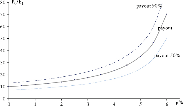
Exhibit 12.12 P/E trend with respect to the growth rate
Exhibit 12.12 is built on the basis of parameter values commonly accepted by financial analysts:
 (in nominal terms)
- Duration of growth: unlimited
In Exhibit 12.12, the graph showing the ![]() trend (the
trend (the ![]() ratio and the
ratio and the ![]() ratio have the same profile in a no-leverage scenario) is obtained on the basis of the relationship reported in section 12.3:
ratio have the same profile in a no-leverage scenario) is obtained on the basis of the relationship reported in section 12.3:
To be precise, the bolded line refers to the dividend payout ratio, which is considered normal in the industry (70 percent). Its profile mirrors the reinvestment rate of return: holding the payout ratio constant (equal to 1 – Share of reinvested earnings), the trend of the growth rate only depends on the rate of return. Using the Gordon model, we know that the growth rate is equal to the product of the ROE times the rate of reinvestment of profit:
where:
| g | = | growth rate |
| b | = | reinvestment rate (1 − Payout ratio) |
| ROE | = | return on equity |
These simple considerations allow us to project point B on the curve in Exhibit 12.12. B has an interesting meaning, as it is identified by the growth rate g*, for which the rate of return is equal to the opportunity cost of capital. Assuming a payout ratio equal to 70 percent (and a corresponding reinvestment rate equal to 30 percent) and a ROE of 7 percent (equal to the value of ![]() in the example), we get to:
in the example), we get to:
Holding the assumption that ![]() at point B, growth neither creates nor destroys value. The multiple obtained by projecting B onto the vertical axis, valued at 14.28, is equal to the price–earnings ratio in a steady-state scenario with no reinvestment. If profits were fully distributed, the multiple would become:12
at point B, growth neither creates nor destroys value. The multiple obtained by projecting B onto the vertical axis, valued at 14.28, is equal to the price–earnings ratio in a steady-state scenario with no reinvestment. If profits were fully distributed, the multiple would become:12
By increasing or decreasing the payout ratio, the graph shifts upward and downward, respectively.
In particular, considering the previous comments, we can choose different values for the payout ratio and identify the corresponding points g1, g2, …, gn that equal the value of growth when the return on new investments is equal to the cost of capital.

Also, projecting g1, g2, …, gn on the lines corresponding to the different payout ratios leads to the points B1, B2, …, Bn, which lie on the same straight line corresponding to a multiple equal to 14.28. This is a consequence of what has already been discussed: when the return on new investment is equal to the cost of capital, the P/E multiple is a function of a unique variable, Keu.
Finally, the 14.28 multiple identifies, regardless of the payout ratio, a line of separation between companies that create value and those that destroy value through the reinvestment of part of their profits. These considerations are valid only for firms that belong to the same risk class (i.e., ![]() is held constant) and that are characterized by the same perpetual growth model.
is held constant) and that are characterized by the same perpetual growth model.
12.8.2 Multiples in the Technology Sector
Exhibit 12.13 has been created using parameters that usually describe industries with a higher-than-average risk profile. In particular, the graph refers to the trend between the P/E ratio and growth in technology companies.
Commonly assumed parameters are:
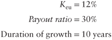

Exhibit 12.13 Trend of the P/E ratio with respect to the growth rate
In comparison to Exhibit 12.12, the scale of growth is much greater. The companies under consideration can exploit development opportunities. The growth period, in this case, must be limited according to the size of the market and the level of competition. In Exhibit 12.13, the multiples have been calculated using the temporary growth model. In particular, the growth (g) period is assumed to end after 10 years and to be followed by a 10-year-long steady-state world (![]() ).
).
Comparing Exhibits 12.12 and 12.13, we can easily notice that the effect of growth on the value of the multiple is much more limited in the high-tech sector. This is due to two factors:
- Growth is assumed to be perpetual in the utilities sector, while it is limited to a 10-year period in the technological sector.
- Using the same hypothesis in the utilities sector, every percentage point of growth generates value. Since the risk in utilities is lower,
 is lower, too.
This example allows us to draw some conclusions on the analysis of multiples in industries impacted by relevant innovations.
Since in this industry business plans usually present a high growth rate (and historical results, which are the basis for the calculation of growth, are often modest), the most important element in the valuation becomes the appreciation of the expected cash flow profile.
In these cases, the two-stage growth models discussed in Chapter 7 are not sufficient to deal with the phenomenon. It is instead better to use three-stage growth models:
- The first stage, limited to the first 5 years, represents the extension of the business plan.
- The second stage, limited to 10 years, refers to the depletion of the development cycle of the business area.
- The third stage is characterized by a growth rate not higher than the long-term GDP growth rate.
We have to say that the growth of cash flow, which is the correct parameter to calculate the company's value and to analyze its multiples, is sometimes confused with the market growth rate. This must be avoided, as it assumes that there is no competition and that all the companies in the industry are faced with the same opportunities. Some analysis on the value taken by multiples in developing industries in the speculative market phases show that common mistakes in valuations are due to analysts' superficial behavior, who often consider market forecasts as the basis to calculate the company's growth rate.
12.9 RELATIONSHIP BETWEEN MULTIPLES AND GROWTH
The relationship between growth and multiples helps to interpret differences in the values of multiples for the selected firms. The relationships explored in Exhibits 12.12 and 12.13 between multiples and growth forecasts are reliable if and only if these conditions take place:
- The duration of growth is uniform. This means that the same growth model is adopted for all the selected companies.
- The risk level is uniform. In other words, even if the selected companies operate in the same business area, there are no relevant differences in the business model, quality of management, competitive position, and so on.
- Companies use their undistributed profits in projects characterized by equivalent expected returns.
Since not all of these conditions always hold, analysts cannot simply accept the relationship between multiples and growth expectations shown in the previous two examples.
A procedure that can help enhance the analysis between multiples and analysts' growth forecasts of a selected sample of companies is to map the relationship in a graph. Exhibit 12.14 is an example of this.

Exhibit 12.14 Map of multiples with respect to growth
This map represents the characteristics of the selected companies; it can be done with respect to:
- Elements that can differentiate the companies with respect to their risk profile
- Duration of growth
- Strategies and objectives disclosed by management in terms of returns in the short and long term
- Consistency between the firms' growth forecasts and their resources
If the comparable companies can be positioned on the map on the basis of the aforementioned factors, the map becomes a useful instrument to also position the company under valuation.
Mapping multiples represents a qualitative approach, which could eventually help analysts with the identification of the most appropriate criteria to be used in the company's valuation. In particular, mapping is useful to:
- Assess whether the calculation of multiples is a rational and sensible decision for the firm's valuation.
- Segment the selected group of companies to improve the comparability with respect to the company under valuation.
- Use procedures to calculate multiples based on the use of a regression or extrapolation.
12.10 PEG RATIO
Portfolio managers often compare the PE multiple to the analysts' growth forecast in order to find under- or overvalued stocks. The PE/g (PEG) ratio is generally used as a useful measure that is standardized with respect to growth.
In fact, the PEG index is rarely used in business valuations. The procedure is based on multiples adjusted with respect to growth according to the following relationship:
- mc = current multiple (with respect to 200x results) of comparable firms
- g′ = growth rate expected for the comparable firms for the period between 200x and 200y
- g″ = growth rate for the company being valued for the period between 200x and 200y
This procedure has been used to evaluate Internet companies and it has usually been applied to sales multiples (EV/Sales). Analysts used this method because the growth prospects of Internet companies were significantly different from country to country. Since the most comparable companies were listed in the United States, multiples calculated with respect to US companies could be modified to be applied to other Internet companies located in different countries.
With this approach, adjusted multiples would represent an estimation of the values we would have obtained if the selected companies' expected growth rate had been equal to the one of the valuated firm. Even if the adjusted method is useful, it is unfortunately characterized by some theoretical approximations and pitfalls. The adjustment of the multiple is simply based on the assumption that the risk profiles of both the comparable companies and the company under consideration are not influenced by the expected growth rate.13
12.11 VALUE MAPS
Building on the analysis of multiples' fundamentals, an alternative approach to relative valuation (especially popular for financial companies) consists in regressing a multiple such as the P/BV against a measure of profitability like the ROE for a panel of comparable companies. Usually, a simple linear regression is performed; if the regression line fits reasonably well to the set of data—the coefficient of determination (R-squared) is assumed as an indicative measure of the fitting14—the regression line itself can become a valuation or investment selection tool. The basic intuition of this approach is that the profitability is the major driver of market value of companies; therefore, a certain level of profitability should affect (in a linear and/or nonliner manner) the multiple. The regression is usually presented through graphs called value maps. Exhibit 12.15 shows, for example, a least squares regression for 44 comparable companies in the financial sector. The first regression is linear and the second is quadratic. They both seem to have a good fit for the data: the R2 is 0.48 for the linear model and 0.54 for the quadratic one. The coefficients indicate that the quadratic curve fits the data better than the linear one, so it's the regression to prefer (we do not discuss here the theory and procedures for curve fitting, but most spreadsheet packages currently in circulation include functions and algorithms to perform regressions and best-fitting analyses).
From an investor's point of view, the value map can be a useful tool to make investment decisions. Companies below (and significantly distant from) the regression line (or curve) can be considered, all the rest being equal, as undervalued and therefore as investment opportunities. Symmetrically, firms above the regression line appear to be overvalued and are therefore potential divestment or shorting candidates. Finally, the companies positioned on the line or close to that, emerge as fairly valued by the market and they appear to deserve a “neutral” investment recommendation. Of course, value maps just offer a partial view of the value determinants and they overlook other potential factors impacting the multiple. In the previous example, the evidence is that ROE is an important element for multiples but definitely not the only one. Statistically, half of the variance of the data remains unexplained or, to be more precise, could be explained by factors different from ROE.
Other than a tool for portfolio decisions, value maps can be used as an equity valuation technique. For example, assume that the 44 companies examined before are all adequately comparable for a target we would like to evaluate. The regression equation expressing the quadratic curve for the comparables is:
Knowing that the companies we aim to value have an ![]() , by using such input in the equation we get a P/BV of 1.93. Considering then that the current book value of the equity for the company is €3,924 million, we conclude that a fair valuation for the equity would be €7,587 million.
, by using such input in the equation we get a P/BV of 1.93. Considering then that the current book value of the equity for the company is €3,924 million, we conclude that a fair valuation for the equity would be €7,587 million.
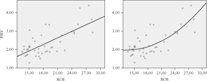
Exhibit 12.15 Value maps for a sample of financial companies
When valuing a company the regression of the P/BV multiple against ROE is a very popular pick, but other combinations of variables may perform equally or even better. In terms of multiples, the P/E ratio is usually an alternative good candidate while in terms of profitability measures possible choices are: the return on average equity (ROAE) that is the return over the mean of the current and expected equity book value, and the return on assets (ROA) that is the ratio between the operating income and the total assets.
Some warnings have to be cast about the preparation of value maps. The actual comparability of the companies included in the regression is key as usual. A trade-off between the number of comparables and the strictness of the comparability criteria does apply and has to be managed by the valuator. As shown in the previous example, a linear regression is not always the best approach: the goodness of fit of nonlinear solutions should be explored in order to catch more precisely the nature of the relation between multiple and fundamentals. Finally, as for ROE and other profitability measures, the use of expected values rather than current ones is recommended. In fact, expected values do incorporate the growth element as well and so they add to the explanatory power of the regression. Actually, in case the industry analysis shows that the companies are expected to experience different growth patterns, the regression of the multiples may be run against the growth rate itself (g).
If the panel of comparables is rather large, an alternative valuation strategy is to perform a regression of the multiples against more than one fundamental, thus overcoming the major limitation of value maps. For example, the regression may include the multiple as a dependent variable and several fundamentals—such as ROE, expected growth, beta (a proxy of risk), or the level of capitalization—as independent variables. Other additional firm-level variables may be added to understand more granularly what elements do have an impact on the multiple. For example, we performed a regression using the data from the 136 largest listed US banks in 2012. The multiple (dependent variable) considered is the current P/BV while the assumed multiple determinants (independent variables) are the long-term growth rate (gs) forecasted by analysts, the level of capitalization (TR), the stock beta, and the return on the average book value of equity (ROAE). By running the regression, we obtain:
The R2 of the regression is 49.60 percent, and the t-test statistics are shown under the independent variables. The signs of the determinants are coherent with predictions: growth, level of capitalization, and profitability contribute positively to the P/BV ratio while the level of risk (reflected in the beta) has a negative impact. From a statistically point of view, the variables Growth and TR do not appear to be significant.15 Actually, if we rerun the regression using only the last two variables, we obtain a result with R2 of 48.71 percent, not far from the previous result, but in this case we have a more parsimonious estimation model.
This sort of augmented regression can be used in two ways, depending on the valuation purpose. On the one hand, it allows the identification of apparently undervalued or overvalued companies, thus suggesting possible investment (long or short) opportunities. On the other hand, the coefficient of the regression may be applied to firm fundamentals to compute the multiple and thus estimate the equity value.
APPENDIX 12.1: P/E WITH GROWTH
multiplying and dividing by ![]() ;
;

adding and subtracting ![]() ,
,


since ![]() , the following expression can be rewritten as:
, the following expression can be rewritten as:

simplifying the first term ![]() and collecting
and collecting ![]() in the second term:
in the second term:

collecting ![]() in the second term:
in the second term:

____________________