
Chapter 13
Multiples in Practice
13.1 A FRAMEWORK FOR THE USE OF STOCK MARKET MULTIPLES
The practical considerations about of market multiples presented in this chapter are based on the principles discussed in Chapter 12. We aim at providing the key tools to apply the relative valuation via multiples, and to critically assess relative valuations carried out by third parties. Our discussion is organized in the following way:
- How to build the sample of comparable companies in the industry under consideration.
- How to define a short list of companies comparable to the one being studied.
- How to “clean” the sample.
- How to assess the validity and actual comparability of multiples.
- How to cross-check the consistency of different multiples, business models, and value drivers.
- How to choose the proper multiples for the valuation.
13.1.1 Building the Panel of Comparables
The sample of comparable companies can be selected using the main international databases (i.e., Bloomberg and Datastream are the most popular), which include information about the industry they belong to, the kind of activity they perform, their degree of diversification, as well as all the economic and financial information required to calculate their multiples.
The first step of the analysis consists of the identification of the industry the company works in. The direct competitors of the company—when available—are usually good candidates in terms of comparability. Bear in mind that geographical markets of reference and countries where shares are listed are not necessarily the same, as in the case of a European company listed in a non-European stock market.
Once the comparable companies are identified, their data are downloaded for every selected company to calculate their respective multiples and test their significance. Such data should include stock-market capitalization, the number of shares outstanding, balance sheet items, and information about the companies' degree of diversification (revenue by business area).
13.1.2 Making a Short List of Comparable Companies
Usually, not all the companies selected in the first round of analysis are valid comparables or can express meaningful multiples. The reasons why this happen are two:
- The industry classifications adopted by the data providers are not always correct or consistent. For instance, companies that manage only trade activities are not distinguished from those that carry out manufacturing activities. This problem often emerges when the industry comprises a limited number of companies.
- Companies are classified according to their main activity. However, the company may run other businesses even completely unrelated to the main one. This situation may significantly bias the multiple expressed by the potential comparable.
Presence of Other Businesses
When the comparable company run also unrelated business, the decision to be made is whether that company is an appropriate comparable or not.
The main principle that drive the selection of the valid comparable companies is the relevance of the activities unrelated to the core business. Such relevance should be evaluated at both sales level and operating margin level.
As a rule of thumb, a company is a potentially sound comparable if the main business has a weight of at least about 70% on the total revenues or operating margin. If the core business has a lower weight, it is generally appropriate to exclude this company from the sample.
However, when the other businesses instead represent complementary activities to the core one, the company's exclusion from the sample is not always recommended. An example can prove useful.
Many European public utilities companies made in recent years relevant investments in the telecommunication and financial services businesses in order to exploit existing commercial relationships with clients and existing distribution networks. These choices implied a change in their strategy, which initially was been rewarded by the market in terms of share prices.
In such a case, it was generally correct not to exclude from the sample the public utilities that underwent a diversification strategy. By keeping the diversified utilities in the sample even if the company to be valued was a “pure” player, the computed multiples were able to embed the value associated with a potential expansion of the business model.
13.1.3 Cleaning the Sample
Cleaning the sample aims at eliminating meaningless multiples, which would be likely to bias the average multiple value.
These multiples lack economic meaning when the company is not in a balanced and sustainable situation. When the current or expected results are too low or even negative the multiples based on net income, the EBIT, or the EBITDA are not meaningful.
A simple rule for discovering anomalies in the multiples is to compute both the values of “direct” multiples (P/E, EV/EBIT, EV/EBITDA) and of “indirect” multiples (EV/Sales, P/BV). If the two categories of multiples are inconsistent, the analyst should explore in depth the reasons for such situation and possibly discard the companies that show inconsistent values.
13.1.4 Checking the Validity of the Multiples
Once the sample has passed the first cleaning phase, further checks have to be run and adjustments have to be made in order to get meaningful and reliable valuations.
The main circumstances that require further analysis and adjustments are summarized in list below.
- A. In depth analyses regarding the validity of multiples in cases where:
- Results are influenced by significant positive or negative extraordinary items.
- Current taxes are balanced by tax credits.
- The net financial position is negative (i.e., there is net liquidity);
- Within groups, minorities hold important stakes in the consolidated companies.
- The company has issued convertible bonds and warrants.
- Changes in capital have occurred recently.
- B. Further analyses regarding multiples' comparability:
- Companies adopt different and inconsistent accounting principles.
- Companies are subject to different tax systems.
- Companies have significantly different financial structures.
Each of the points above will be discussed briefly in the following paragraphs.
13.2 THE SIGNIFICANCE OF MULTIPLES
13.2.1 Extraordinary Items
The need to calculate P/E multiples excluding results from extraordinary items is rather straightforward and does not need additional comments.
It is worth mentioning that measures such as the EBIT and the EBITDA can also contain extraordinary components that are not always highlighted in the notes reported in financial statements. For instance, in industrial and commercial companies, income derived from an extraordinary disposal of goods (i.e., the fire sale of inventory) can influence operating results in a significant way. The same can occur with exchange rate gains or losses due to extraordinary commercial transactions, and so on.
13.2.2 Tax Credits
Another frequent cause of distortion that needs to be corrected is the existence of tax credits (previous tax-deductible losses, reductions in tax rates or of the taxable income derived from temporary facilitating laws, etc.).
The results from which multiples are calculated should usually be expressed net of the normalized tax liability calculated using the marginal tax rate. This is due to the fact that tax benefits are usually just temporary. It has to be mentioned that in normal market efficiency conditions, market capitalization should include the present value of the expected tax benefits.
For these reasons, analysts generally perform a double adjustment: the first is a normalization of the tax burden while the second concerns market capitalization. The example shown in Exhibit 13.1 can clarify this procedure.
We assume that companies A and B are completely similar in the following table; B can, however, exploit tax credits with a present value equal to 2,000. Therefore, its market capitalization turns out to be higher than A's. The adjustments reported in the table allow us to obtain identical P/E values for the two companies.
Exhibit 13.1 The relevance of tax credits
| Company A | Company B | |
| Earnings Before Taxes | 1,000 | 1,000 |
| Corporate Taxes (37%) | 370 | 0 |
| Other Taxes | 100 | 100 |
| Net Income | 530 | 900 |
| Equity Value | 7,950 | 9,950 |
| Unadjusted P/E | 15 | 11 |
| Adjusted Result (Tax rate = 37%) | 530 | 530 |
| P/E with Adjusted Net Income | 15 | 18.7 |
| Present Value of Tax Credits | – | 2,000 |
| P/E with Adjusted Equity Value and Adjusted Net Income | 15 | 15* |
* (9950 − 2000)/530
13.2.3 Positive Net Financial Position
With a significant positive net financial position, multiples can turn out to be distorted. As a matter of fact, we can assume that market capitalization is equal to the sum of the company's base-value, represented by its core activity, and its liquidity surplus.
Consequently, analysts generally subtract the value of net liquidity from the company's capitalization and the financial revenues to which it refers net of the respective tax effects from net income.
However, the such procedure is not always appropriate. If liquidity is created through an increase in capital, particularly through an initial public offering, and is planned to finance an investment program, it is possible that the valuation of the project reflected in market capitalization assumes that the liquidity will be used for the program development.
Consequently, in this case, the capitalization adjustment according to liquidity can yield biased results.
The market capitalization adjustment according to liquidity should therefore be based on the assumption that liquidity forms a surplus asset in every sense.
13.2.4 Group Structures
The majority of difficulties that are going to be discussed hereafter do not apply if a holding company owns 100 percent of the capital of its subsidiaries. As a matter of fact, group results are entirely referable to the shareholders of the holding company.
However, if there are minority shareholders in the subsidiaries, part of the group results belongs to them.
The consolidated financial statement allows us to find what belongs to third parties by referring only to the last line of the income statement: the net income respectively of the parent company's shareholders and of the minority shareholders in the subsidiaries. Nevertheless, this is not possible for intermediate results (such as the EBITDA, the EBIT, cash flows).
As a consequence, there is no consistency between the market value of the listed parent company and intermediate results which reflect the performance of the entire group (thus including third parties interests).
The only multiples for which the homogeneity prerequisite is respected are the Price/Earnings ratio calculated without net income adjustments and the Price/Book value ratio.
This distortion is unavoidable as it is not clear whether and how the market value of a holding company also “captures” a part of the value referable to third parties. Among the different methods that aim at limiting this distortion, the procedure based on adjusting the holding company's market capitalization is widely appreciated.1 Two different options are possible:
- The addition of the book value of the minority shareholders' equity to the capitalization of the holding company;
- The addition of the estimated value of the minority shareholders' equity to the capitalization of the holding company.
Analysts generally prefer the former option for the sake of simplicity.
By doing so, third parties' equity is perceived as financial debt.
13.2.5 Capital Increases
When an increase in equity occurs close to the period in which the multiples are calculated, it is necessary to verify that the consistency between market prices and the company values used in the multiples still exists.
This issue arises because a capital increase leads to an immediate effect on the market capitalization of the company due to the capital increase and on the unit price of the stock. Nevertheless, the effect on the results is deferred.
In the case of right issues, the intensity of the effects produced by the capital increase depends also on the methods used in its implementation and, particularly, on the gap between the price of the new shares issued and the market price in the period prior to the transaction.
This statement can be better explained by precisely showing the effects of a capital increase on market capitalization and on a listed company's share prices.
Market Capitalization
It can be assumed that a company's market capitalization after a capital increase changes in the following way:
Share Prices
The price after the transaction (![]() ) should correspond to the weighted average of the price of the old shares and the subscription price of the new ones. The following equation expresses this concept:
) should correspond to the weighted average of the price of the old shares and the subscription price of the new ones. The following equation expresses this concept:
where:
| TERP | = | Theoretical Ex-Rights Price; that is, the market price after the exercise of the right to subscribe new shares |
| = | market price before the exercise of the right | |
| = | price of the new shares issued | |
| = | number of old shares | |
| = | number of new shares issued |
The effect on the unit share price is called the dilution effect in financial jargon. It depends on the gap between ![]() and
and ![]() : the transaction would not impact
: the transaction would not impact ![]() if and only if the issue happened at a price equal to the market price (
if and only if the issue happened at a price equal to the market price (![]() ). If the issue price is instead significantly lower than the market price, the dilution effect can be very relevant. In the case of a free shares distributed to shareholders (
). If the issue price is instead significantly lower than the market price, the dilution effect can be very relevant. In the case of a free shares distributed to shareholders (![]() ), we can observe the maximum dilution effect.2
), we can observe the maximum dilution effect.2
13.2.6 Convertible Bonds, Warrants, and Stock Options
If convertible bonds have been issued, the company has acquired financial resources that have been invested and have contributed to the generation of results. When the conversion right is exercised, the same results will have to be divided among a greater number of shares.
Accepting the assumption of efficient markets, investors should take this possibility into account and make informed long-term choices based on “diluted” earnings per share, cash flows, EBIT.
Consequently, multiples should also be calculated with respect to the updated value of earnings per share after the conversion of any shares and not the current EPS. Diluted earnings per share are usually calculated and reported by the main databases.
We should highlight that the calculation of diluted earnings per share is not always easy: as a matter of fact, it is often impossible to predict whether subscribers will exercise their conversion rights. For example, if the conversion price is higher than the current market price of the stock, it will be more advantageous to not exercise the conversion rights and wait instead for the repayment of the bonds.
If warrants exist, the problem becomes more complex. Contrarily to the case of convertible bonds, financial resources will flow into the company only in the future, at the moment of subscription of the new shares to which the rights refer. The issuance of warrants leads to the same adjustment issues we discussed with regard to an increase in capital even though the capital increases are only “potential” in this case.
Stock option plans can create dilution effects that are completely equivalent to those discussed in the previous cases. This depends on the subscription conditions foreseen in the plans.
13.3 THE COMPARABILITY OF MULTIPLES
13.3.1 Accounting Principles
The comparability problem is more serious when the sample is composed of companies from countries that have different accounting principles. For example, the European accounting principles are still substantially different from those used in Anglo-Saxon countries, as well as from those adopted in the Far East.
Even if all the selected companies are in the same country, the results of some business areas are often significantly influenced by the choices carried out in the financial statement. For example, it is usually necessary to adjust the income statements of the companies in the sample using uniform criteria to calculate the provisions for risks, and to value their financial investments.
13.3.2 Different Tax Systems
The tax rate—which expresses the impact of taxes on the company's income—measures that part of the income taken from the company and transferred to the public administration. Therefore, holding EBT constant, different tax rates lead to different equity values and therefore different market capitalizations.
This problem has particular relevance when multiples like the EV/EBIT, the EV/EBITDA, and the P/BV are compared. As a matter of fact, the denominators in these ratios are all gross of the tax burden. In the P/E ratio, however, the denominator is an item net of taxes and the tax system bias is therefore generally neutralized.
13.3.3 Different Degree of Leverage
The problems of comparability with respect to companies in the sample that are more levered than others or are characterized by a significantly different average financial position from the one of the company under consideration, have been widely discussed in previous chapters.
The use of adjustment formulas that are technically correct is not always appropriate because of the uncertainty surrounding the real possibility of exploitation of tax shields linked to the deductibility of interest.
Nevertheless, leverage adjustments can help explain differences in the values of multiples in some specific instances. As already explained, these adjustments are particularly useful in the following cases:
- In industries where future results are highly predictable and stable over time, therefore leading to a high level of credibility surrounding the effective use of tax benefits
- When the tax benefits are particularly high
13.3.4 Searching for Significant Relationships between Multiples, Business Models, and Value Drivers
Once the sample has been selected correctly and the adjustments discussed in the last two paragraphs have been carried out, the observable differences in the multiples can be finally analyzed from a pure business perspective.
The reasons why some companies belonging to the same sample are valued more by the market have to be understood. As a matter of fact, the differences in valuation that are observed must mirror beliefs on the companies' ability to enhance their earnings per share. The key point is then to understand what value drivers are used by the market to evaluate this capability and how the selected companies are positioned with respect to the most relevant value drivers.
The final goal is to rank the sample companies and the company being valued according to the validity of the business model itself and the deployment of differential resources/advantages with respect to competitors.
This kind of analysis requires a deep knowledge of the industry. This is also a reason why the big investment firms tend to build teams of specialized analysts that cover only one or few industries.
13.4 MULTIPLES CHOICE IN VALUATION PROCESSES
The process that has been explained so far concludes with the definition of a handful of multiples that will have to be applied to the firm that is being valued.
This choice represents the summary of the analysis that has been accomplished in the previous stages and requires the solution to the following problems:
- The definition of a reference period for the calculation of the market price of comparable companies: Analysts often prepare spreadsheets where the multiples are calculated both based on the last available price and on the average price of the previous periods. The choice of the reference period generally occurs in the last stages of the analysis. As a matter of fact, the information collected can give useful hints for the interpretation of the behavior of the market for the stocks of the companies in the sample.
- The selection of the multiples for the company's valuation: Analysts generally use programs that calculate all the multiples that have been discussed in the previous chapter. However, for the purpose of the valuation, the least meaningful multiples are rejected.
- The calculation of the value synthesizing the information derived from the selected multiples.
13.4.1 Time Horizon
The logic of the market approach would require the market prices used in the multiples calculations to be taken from time periods close to the reference date of the valuation. It is, however, often preferable to calculate multiples based on the two months, half year, or even annual average of prices prior to the valuation date.
Such a choice is motivated by the concern that market prices are affected by anomalies or manipulations. By extending the observation period, the anomalous values will instead tend to balance themselves out.
It does not make sense to create a single rule on this topic. This choice has to be made on a case-by-case basis depending on the level of trading volumes, which are considered an indicator of the representativeness of the prices present in the market.
13.4.2 Selection of Multiples
Financial analysts usually perform valuation processes using a grid formed by two to four multiples.
For the valuation of industrial companies, the most widely used multiples are:
- EV/EBIT
- EV/EBITDA
- EV/Sales
The reasons for this choice are most likely due to the fact that the P/BV multiple is less meaningful in manufacturing sectors, while the P/E ratio is generally more sensitive to the criteria used in the preparation of the company's financial statements.
Nonetheless, it is crucial to mention that there are relevant exceptions to this rule.
In the valuation of banks and insurance companies, multiples of the book value and multiples of specific economic value drivers representing the performance of the companies that belong to that particular industry (i.e., the net interest income, net fees and commissions, net trading revenues, etc.) are used more frequently.
In the search for the most suitable multiples, it can be useful to carry out an empirical comparison that shows the ability of different multiples to explain the value of the target company. As a matter of fact, it is possible to assess if the market implicitly attributes the ability to estimate the price of a company to a particular variable. The best way to do this is to run an analysis on the correlation between the multiples and the particular variable under consideration for the companies in the sample. The greater the correlation, the more the multiple is able to capture the company's market price.3
13.4.3 Synthetic Value of the Selected Multiples
The problem consists in summarizing the various values of the multiples of the sample companies into a unique value.
There are different ways to do so. We list a few methods, based on their frequency of use:
- Computation of the multiple average and median. The median can generally be considered as a satisfactory choice for those industries where companies have substantially uniform business models. In this case, the differences observed between multiples can be traced back to the sample companies' growth perspectives and their capability to generate superior performances. A further condition is that the company that is being valued is an average player in the market with respect to the aforementioned factors.
- Segmentation of the sample in homogeneous subcategories. A technique that is frequently used by financial analysts is the regrouping of the sample companies into two or three subcategories to enhance the firms' comparability with the company that is being valued. The segmentation should occur based on objective criteria, such as size, international presence, ownership of particularly important brands and technologies, etc. Analysts should then understand to what subcategory the company under consideration belongs. The value of the benchmark multiple is finally obtained calculating the arithmetic average of the multiples of the companies that belong to this subcategory.
- Procedures based on extrapolation. In some cases, the analysis of sample multiples allows us to find relevant relationships between the values of the indices and the specific value drivers. The procedures described in the previous points might not be entirely convincing in cases when, for example, the positioning of the valued company is very different from the one of the other sample companies. In these situations, analysts sometimes use techniques that are based on the interpolation or the extrapolation of the multiples observable in the sample.
Finally, the estimated value of the company is obtained by calculating the simple average of the values derived from the use of each multiple as applied to the company to be valued. If the analysts thinks that some multiples are more relevant than others, weighted averages might be used instead.
13.5 ESTIMATION OF “EXIT” MULTIPLES
The problem of estimating exit multiples is relevant in two instances:
- For the terminal value estimate, which is the value of the company at the end of the analytical projection period of the cash flows (
 ) in the valuation methods based on analytic DCF models.
 - For the estimate of the divestiture value in acquisitions with short time horizons (
 ), typically realized by private equity funds.
In both cases, analysts have to form forecasts on the evolution over the time of the multiples calculated on the basis of the actual stock prices.
In order to face this problem rationally, it is convenient to split it up into two parts:
- The estimate of the average industry multiples at

- The estimates of the multiples of the different companies belonging to the industry at

13.5.1 Industry Multiples at tn
The predictable level of the average multiples in the industry depends on two different factors:
- The attractiveness of the market in which the companies belonging to the specific industry operate with respect to the future period

- The long-term evolution of the average multiples with respect to the entire stock market, which depends on the trend of interest rates and on the attractiveness of risky investments compared to risk-free ones
Some analysts maintain that the value of multiples must necessarily converge to the average value of the multiples calculated over a sufficiently long period (the last 10–15 years). Alternatively, one can calculate the theoretical multiple in the absence of growth that can be obtained as a function of the estimate of the opportunity cost of capital of the sector.
13.5.2 Differentiation Level
After the average multiple of the industry has been calculated, one can move on to the second stage of the analysis that aims at verifying whether the average multiple needs to be adjusted according to elements that differentiate the company that is being valued from the other companies in the same industry.
Such an adjustment is justified if the analyst is able to make credible projections on the cash flow profile for the period following ![]() and therefore for divestiture periods that last no more than three to five years.
and therefore for divestiture periods that last no more than three to five years.
The basic idea is the following: given that the average multiple is an appropriate valuation index for companies that are characterized by results profiles that are similar to the industry average, the companies that are able to sustain higher growth rates than the competitors' should be valued with higher multiples, and vice versa.
The level of correlation of exit multiples can be evaluated through the analysis of the same factors that explain the dispersion of current multiples.
Alternatively, analysts can use the practical insights derived from the theoretical relationship between multiples and expected growth rates.
13.6 AN ANALYSIS OF DEAL MULTIPLES
The analysis of multiples linked to comparable transactions allows us to obtain significant information regarding a company's likely market price. This concept has already been introduced where we discussed the different informational content of stock market and deal multiples.
A main difference between deal multiples and stock market multiples consists of the reasons that can explain the volatility of the values in the group of selected transactions.
For stock market multiples, the volatility is, at least theoretically, the consequence of investors' consideration of the strengths and weaknesses of the companies that belong to the sample from a stand-alone perspective.
On the other hand, the value of deal multiples also depends on the context and specificities of the transaction.
As we will explain better later, the divestiture price is influenced by two types of factors:
- Market factors, such as the competition level between willing buyers and the acquisition values estimated by each of them
- Transaction factors, such as the percentage of acquired capital, payment methods (cash or acquirer's stock), the contractual terms regarding the guarantees given by the seller, mechanisms that tie part of the price to future results (earnouts), the existence of surplus assets that can allow the acquirer to make levered transactions, and so on
Therefore, the analysis of deal multiples requires the collection and interpretation of a certain amount of information regarding transactions that can significantly influence the negotiated price and the value of multiples consequently. We are going to focus on a few elements that are particularly crucial in this analysis.
13.6.1 Percentage of Acquired Capital
Deal multiples have greater significance when the transaction involves the company's entire capital. As a matter of fact, if the control stake is acquired, it is possible that the negotiated price also includes a control premium in addition to the proportional value of the acquired capital.
The possible existence of the premium does not allow for the calculation of the value of the entire capital through a simple proportion as in the following example. Therefore, if the price paid for 60 percent of the capital is 1,200, the value of 100 percent of the company is not ![]() .
.
This problem is not easy to solve because analysts are not able to objectively evaluate the existence and size of the premium; the information provided represents only a guideline to perform this kind of analysis.
When the transaction concerns the acquisition of a qualified minority stake, other problems arise. As a matter of fact, the acquisition of a minority stake can represent a simple financial investment, as in the case of a fund investing in a company with the objective of subsequently divesting from it through an IPO. The minority acquisition could also simply be linked to production or commercial agreements, as in the case of an acquirer who is an industrial operator. Finally, the acquisition of a minority stake is sometimes part of a transaction to acquire control in multiple stages.
In these cases, the significance of the price can change radically. For instance, if the acquisition of the minority interest is part of a broader program of transfer of control, acquirer and seller could have agreed on a price for the entire capital and have split it nonproportionally between the first installment and the following ones for the sake of convenience.
13.6.2 Characteristics of the Acquirer
Deal multiples relative to sale transactions to industrial counterparts are generally higher than multiples of transactions carried out with financial investors.
As a matter of fact, the acquisition prices should include a part of the value expected to be derived from the so-called merger synergies.
We should also highlight that this indicator is disavowed in some cases: As a matter of fact, some private equity funds follow an active entrepreneurial approach, for example, focusing on the creation of value through the aggregation of small and medium-sized firms with the goal of obtaining operating synergies or gaining significant market shares in the industries in which the companies operate.
Using the previously explained investment strategies, these funds can pay higher prices than the stand-alone value of the acquired companies. Consequently, the significance of deal multiples in these cases could be similar to the one of multiples of industrial transactions.
In conclusion, the analysis of deal multiples heavily depends on the characteristics of the acquirer with differences between:
- “Strategic” buyers
- Investment funds with an active/entrepreneurial approach that follow an entrepreneurial approach
- Investment funds that engage in transactions mainly of a (passive) financial nature.
13.6.3 Existence of Surplus Assets
A typical problem that exists when dealing with deal multiples is the existence of surplus assets. As a matter of fact, the total acquisition value is estimated by adding the value of the surplus assets to the acquisition value of the core business.
Consequently, deal multiples will have to be adjusted by subtracting the value of the disposal of the assets that are not functional to the core business from the price paid by the acquirer. It is easy to observe that the same problem can also exist with stock market multiples. However, holding all other factors constant, the need for such an adjustment is lower in this case because the stock market tends to undervalue surplus assets, especially if they are not crucial for cash flow generation.
It is possible, however, that in the case of a transfer of control, the acquirer also considers the money that will be recovered through the disposal of nonstrategic assets.
13.6.4 Payment Methods
Deal multiples are more significant in valuation processes when the acquisition is paid in cash. In many transactions the acquisition occurs instead through the transfer of the acquirer's shares or in a mixed form (shares plus cash).
If the payment method is the transfer of shares, a problem of relative valuation arises: the transaction could have taken place by inflating value of both the target's and the acquirer's shares.
This problem is particularly serious when either the acquirer's or the target company's shares are not listed and therefore no objective benchmark exists.
13.6.5 Earnouts
Another essential element in this discussion is the effective payment terms, which can be fragmented in multiple stages or include earnouts.
As mentioned before, an earnout provision implies that part of the price to be paid depends on the future achievement of the business plan objectives defined during the negotiations.
The price therefore cannot be determined ex-ante. This is a particularly thorny problem in the construction and interpretation of deal multiples. As a matter of fact, the presence of earnouts means that the price paid can vary depending on the results, even if the contracts usually include upper and lower price limits.
Earnout agreements are also usually not disclosed by parties, which makes the adjustment of multiples even more difficult.
13.6.6 Trend of Deal Multiples over Time
The trend of deal multiples over time mirrors the conditions that are created in the control market, which provides either sellers or buyers with a more favorable environment. The model of price formation in that market represents a useful logical tool for the interpretation of the levels reached by deal multiples.
The key factors are the level of competition among willing buyers and the size of merger synergies.
The analysis of the trend of deal multiples over time allows us to reconstruct the historical price paid within specific industries. However, only a true understanding of the current trend can provide a more reliable estimate of deal prices.
Exhibit 13.2 shows the trend of the Price/Book Value multiple with respect to a sample of transactions that took place in the Italian banking industry between 1995 and 2001.
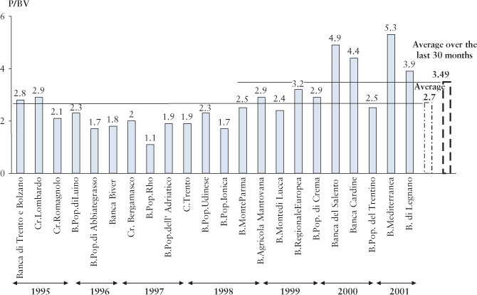
Exhibit 13.2 Trend of the Price/Book value multiple in a sample of transactions in the banking industry
The data shown in the figure allow us to see a significant increase in the multiples over the years 2000 and 2001 with respect to the average over the entire period. Therefore, the simple average over the whole period of time is a misleading indicator of the likely market price for transactions with transfer of control that could be realized in the more recent period.
13.7 THE COMPARABLE APPROACH: THE CASE OF WINE CO.
The discussion of the case presented in this paragraph has the goal of showing a valuation procedure based on multiples and to show the unavoidable approximations and problems that analysts run into in real-life cases.
This valuation example refers to an acquisition transaction of part of the capital of a winery carried out by a private equity fund.
13.7.1 The Logic of the Transaction
The wine market went through some important changes over last decade. High-quality wine has become a status symbol and a product that is therefore subject to a similar treatment as consumer goods. This has stimulated a growing interest in the industry among financial investors, favoring, therefore, a significant increase in the market value of companies holding well-known and historical brands.
The transaction we will discuss here is the acquisition of a 40 percent stake in the capital of a winery that owns important and well-known wine brands. The goal of the investment is to further strengthen the fund's presence in the high-quality products segment also through the acquisition of new wine estates.
The divestiture will occur in about three to five years through the sale in the stock market of the shares acquired by the fund.
The business plan prepared by the management assumes that the new acquisitions will absorb a relevant part of the cash flow and that the new investments will start generating cash flows in about five to seven years, considering the time that is necessary to start production in new vineyards and the waiting period for the ageing of the product.
The net flow that can be distributed through dividends (FCFE) over the plan horizon is therefore relatively low and the investment return is mainly created by the difference between the acquisition price and the offer price in the market for Wine Co.'s shares.
13.7.2 Relevant Information for the Valuation
In the picture we have described, the most relevant information for the fund's investment decision can be summarized with:
- Current multiples (stock market and deal multiples), according to which a bid for the target is formulated
- The value of the multiples of comparable companies estimated considering the expected divestiture period (the exit multiples)
Given the exit mechanism assumed by the fund management (an IPO), only stock-market multiples will be analyzed for the estimation of exit multiples.
13.7.3 The Selection of Comparable Companies
The group of listed comparable companies has been found through research in the Bloomberg database.
Two samples of wineries have been selected: the first one includes only European companies while the second one contains only non-European companies (Australia, United States, Chile, and Canada).
The analyst in charge of the valuation has decided to focus the analysis only on the first sample, considering that the European market is more meaningful for the calculation both of the likely market price of Wine Co. and of the estimate of the amount that can be gained through the sale of the stake that is expected to take place through a public offering in a European stock market.
Exhibit 13.3 shows the characteristics of both the sample of European companies and the target company in terms of sales, number of hectares of vineyards owned, and profitability. Moreover, we can also see the sales breakdown with respect to quality, type of product (white and red wines), and export shares.
A first look at Exhibit 13.3 suggests that the last two selected companies have to be excluded from the group of comparable companies because they are mainly commercial companies. The residual sample is composed of five Spanish companies with a production that mainly includes medium–high quality red wines.
Exhibit 13.3 Characteristics of comparable companies (sample of European companies)
| Current data (€m) | |||||||||
| Firm | Nationality | Currency | Hectares owned | Sales | EBITDA | EBIT | EBITDA (% sales) | EBIT (% sales) | |
| Comp. 1 | Spain | Euro | 1,016 | 202.5 | 28.1 | 21.6 | 13.88% | 10.67% | |
| Comp. 2 | Spain | Euro | 200 | 13.3 | 5.5 | 4.5 | 41.35% | 33.83% | |
| Comp. 3 | Spain | Euro | 120 | 57.6 | 23.0 | 26.9 | 41.11% | 32.61% | |
| Comp. 4 | Spain | Euro | 500 | 30.5 | 11.6 | 9.9 | 38.03% | 32.46% | |
| Comp. 5 | Spain | Euro | 150 | 43.2 | 5.4 | 3.2 | 12.50% | 7.41% | |
| Comp. 6 | Germany | Euro | n.a. | 232.4 | 12.8 | 8.7 | 5.51% | 3.74% | |
| Comp. 7 | Germany | Euro | n.a. | 251.2 | 24.4 | 10.1 | 9.71% | 4.02% | |
| Target firm | Italy | Euro | 30 | 55.0 | 17.0 | 15.0 | 30.20% | 27.10% | |
| Breakdown sales for quality of produced wine | |||||||||
| High quality | Average quality | Low quality | Firm | Breakdown sales for geographical area | Kinds of wine produced | ||||
| Comp. 1 | 68% | 30% | 2% | Spain: 64.0%, other: 36.0% | Red wines | ||||
| Comp. 2 | 47% | 37% | 16% | Spain: 82.9%, other: 17.1% | Red wines | ||||
| Comp. 3 | 88% | 12% | Spain: 29.5%, other: 70.5% | Red wines | |||||
| Comp. 4 | 70% | 30% | Spain: 84.9%, other: 15.1% | Red wines | |||||
| Comp. 5 | 70% | 30% | Spain: 86.1%, other: 13.9% | Red wines | |||||
| Comp. 6 | n.a. | Germany: 100.0% | Wines and sparkling wines | ||||||
| Comp. 7 | n.a. | Germany: 57.6%, France: 22.0%, East Europe: 20.4% | Sparkling wines | ||||||
| Target firm | 60.0% | 20.0% | 20.0% | Italy: 40.0%, USA: 60.0% | Red wines | ||||
Therefore, Wine Co. and the selected companies are sufficiently similar to justify a comparative valuation. Despite their similarity, some differing elements still exist that call for further analyses. They include the following facts:
- Wine Co.'s number of vineyard hectares and sales are lower than the selected companies'. As a matter of fact, Wine Co.'s land properties are owned directly by the family that controls the company. Therefore, Wine Co.'s book value is unbalanced with respect to the sample companies. However, this is not considered particularly important for the valuation for many different reasons. First, the business plan anticipates the acquisition of some agricultural properties that will allow Wine Co. to go to the market with an important vineyard property. Second, the company controls the management of the vineyards through 20-year rental agreements and is therefore able to assure standards of quality over a prolonged time horizon.
- The sales breakdown according to geographical areas shows a high degree of concentration in the US market. This can be seen as a positive fact considering the US market's higher growth rates compared to the European one, but it can also be a peculiar risk factor in comparison with the selected comparable companies. As a matter of fact, some analysts believe that the US market will be characterized by increasing competition driven by national producers (i.e., Californian wines) and by Australian and Chilean producers.
Exhibit 13.4 European companies multiples
| Price | |||||||||||||
| Firm | Currency | Current price | Average 6 months | Minimum 6 months | Maximum 6 months | Stock number (m) | Average market cap | Floating shares (m) | Net debt | TEV | |||
| Comp. 1 | Euro | 15.70 | 14.68 | 10.80 | 16.00 | 17.8 | 261.1 | 10.8 | 57.4 | 318.5 | |||
| Comp. 2 | Euro | 8.40 | 8.88 | 8.40 | 9.50 | 5.4 | 48.3 | n.a. | 17.9 | 66.2 | |||
| Comp. 3 | Euro | 27.19 | 24.04 | 19.50 | 28.50 | 7.7 | 185.8 | 4.8 | 39.3 | 225.1 | |||
| Comp. 4 | Euro | 13.35 | 13.57 | 13.00 | 15.00 | 14.3 | 193.4 | 3.2 | 17.9 | 211.3 | |||
| Comp. 5 | Euro | 6.19 | 6.30 | 5.90 | 6.94 | 6.1 | 38.7 | 1.7 | 46.0 | 84.7 | |||
| Sales multiples | EBITDA multiples | EBIT multiples | RN multiples | PN | |||||||||
| Firm | LTM | Ex. t0 | Ex. t+1 | LTM | Ex. t0 | Ex. t+1 | LTM | Ex. t0 | Ex. t+1 | LTM | Ex. t0 | Ex. t+1 | LTM |
| Comp. 1 | 1.6x | 1.4x | 1.3x | 11.3x | 9.4x | 8.7x | 14.7x | 13.1x | 11.9x | 17.4x | 16.2x | 14.6x | 2.0x |
| Comp. 2 | 5.0x | 4.0x | 3.6x | 12.0x | 9.7x | 10.1x | 14.7x | 13.1x | 11.6x | 21.0x | 21.6x | 17.8x | 2.4x |
| Comp. 3 | 4.4x | 3.9x | 3.7x | 10.8x | 9.8x | 8.4x | 13.6x | 12.0x | 10.4x | 12.4x | 11.0x | 10.5x | 2.0x |
| Comp. 4 | 6.5x | 5.2x | 5.4x | 18.2x | 14.0x | 13.9x | 21.3x | 15.7x | 21.5x | 21.2x | 19.9x | 19.3x | 3.4x |
| Comp. 5 | 2.0x | 1.8x | 1.9x | 15.7x | 12.2x | 11.1x | 26.5x | 53.7x | 43.1x | 43.0x | 10.7x | 12.7x | 0.7x |
13.7.4 Analysis of Value Multiples
The data on the value multiples of the selected companies is shown in Exhibit 13.4. The “price” columns show the most recent market price, the average price in the previous semester, the minimum and maximum price in the last six months. The column market capitalization, whose values have been used in the multiple calculations, is based on the average prices of the last semester.
The multiples are respectively calculated on the last available financial statement data (LTM), on the closing forecasts for the current accounting period (Ex. t0), and on the analyst's forecasts regarding the following accounting period (Ex. t+1).
The “floating” column shows the number of shares available in the market. This value can be considered as an indicator of the liquidity of the stock, and consequently, of the significance of stock prices.
A first analysis of the multiples suggests the exclusion of company no. 5 from the sample, as it is not aligned with the other selected companies either in terms of profitability or of financial structure. The financial statements of company no. 5 highlight elevated wine inventory costs that are not easily recovered through products pricing.
The multiples of company no. 5 show the typical asymmetry discussed earlier: the EBIT and EBITDA multiples for this company are very high and out of measure compared to the sample, whereas the sales and book value multiples are very low. This causes us to describe the EBIT and EBITDA multiples as “fake multiples” void of any economic significance.
A further important element that concerns some of the selected companies is the modest gap between the values of the EBIT and the P/E multiples. This fact calls for a check of the effective size of the tax effects. The results of the analysis are summarized in Exhibit 13.5. They show that with a marginal tax rate of 35 percent, two companies face an effective tax rate of 3 percent and 6 percent.
In these particular cases, the size of the current tax levy is mainly explained by the advantages coming from investments and by the company's level of exports.
Exhibit 13.5 Estimates of the fiscal effects
| Calculation tax rate t-3 | Calculation tax rate t-2 | ||||||||
| Firm | EBT | Tax | Net income | Tax rate (real) | EBT | Tax | Net income | Tax rate (real) | |
| Comp. 1 | 16.74 | 5.68 | 11.06 | 33.9% | 19.29 | 6.75 | 12.54 | 35.0% | |
| Comp. 2 | 4.92 | 1.72 | 3.20 | 35.0% | 3.70 | 1.40 | 2.30 | 37.8% | |
| Comp. 3 | 12.30 | 0.71 | 11.59 | 5.8% | 14.64 | 1.32 | 13.32 | 9.0% | |
| Comp. 4 | 8.99 | 2.30 | 6.69 | 25.6% | 10.49 | 1.20 | 9.29 | 11.4% | |
| Calculation tax rate t-3 | |||||||||
| Firm | EBT | Tax | Net income | Tax rate (real) | Theoretical tax rate | ||||
| Comp. 1 | 20.52 | 6.29 | 15.04 | 30.7% | 35.0% | ||||
| Comp. 2 | 3.70 | 1.40 | 2.30 | 37.8% | 35.0% | ||||
| Comp. 3 | 15.89 | 0.93 | 14.96 | 5.9% | 35.0% | ||||
| Comp. 4 | 9.40 | 0.30 | 9.10 | 3.2% | 35.0% | ||||
13.7.5 Tax Rate Adjustments for Multiples
We explained that multiples can turn out to be meaningless when the effective tax rates are significantly different with respect to both the analyzed sample and the target company.
In order to neutralize this effect, the analyst valuing Wine Co. has made the following adjustments:
- The present value of the lower tax rate has been estimated for a five-year period, which is the expected length of the tax concessions. This value has then been subtracted from the company's market capitalization.
- The net result has been recalculated using the full tax rate equal to 35 percent.
Exhibit 13.6 Calculation of the present value of the tax benefits linked to tax concessions
| Firm | EBT | Theoretical tax rate | Theoretical taxes | Real taxes | Theoretical - real | Discount rate(*) | RF present value |
| Comp. 1 | 20.52 | 35.0% | 7.18 | 6.29 | 0.90 | 4.33 | 3.88 |
| Comp. 2 | 3.70 | 35.0% | 1.30 | 1.40 | −0.11 | 4.33 | −0.45 |
| Comp. 3 | 15.89 | 35.0% | 5.56 | 0.93 | 4.63 | 4.33 | 20.05 |
| Comp. 4 | 9.40 | 35.0% | 3.29 | 0.30 | 2.99 | 4.33 | 12.94 |
The estimate of the adjustments has been highlighted in Exhibit 13.6. The table shows the calculation of the tax benefits deriving from tax concessions of the selected companies. It can be observed that these benefits have a significant size in two cases (Comparable 3 and Comparable 4).
Finally, Exhibit 13.7 shows the multiples adjusted with respect to these tax benefits. It is important to highlight that the P/E multiple now has a more coherent trend with respect to the EV/EBIT and the EV/EBITDA multiples. As already mentioned, the adjustments have been made by subtracting the present value of the tax benefits from the market capitalization, and in the P/E ratio case, by “normalizing” the tax burden applying a marginal tax rate equal to 35 percent.
Exhibit 13.7 Adjusted multiples of European companies
| Price | |||||||||||||
| Firm | Current | Average 6 months | Minimum 6 months | Maximum 6 months | Stock number (m) | Average market cap | Adjusted average market cap | Net debt | TEV | Adjusted TEV | |||
| Comp. 1 | 15.70 | 14.68 | 10.80 | 16.00 | 17.8 | 261.1 | 257.2 | 57.4 | 318.5 | 314.6 | |||
| Comp. 2 | 8.40 | 8.88 | 8.40 | 9.50 | 5.4 | 48.3 | 48.8 | 17.9 | 66.2 | 66.7 | |||
| Comp. 3 | 27.19 | 24.04 | 19.50 | 28.50 | 7.7 | 185.8 | 165.7 | 39.3 | 225.1 | 205.0 | |||
| Comp. 4 | 13.35 | 13.57 | 13.00 | 15.00 | 14.3 | 193.4 | 180.4 | 17.9 | 211.3 | 198.3 | |||
| Sales multiples | EBITDA multiples | EBIT multiples | RN multiples | PN | |||||||||
| Firm | LTM | Ex. t0 | Ex. t+1 | LTM | Ex. t0 | Ex. t+1 | LTM | Ex. t0 | Ex. t+1 | LTM | Ex. t0 | Ex. t+1 | LTM |
| Comp. 1 | 1.6x | 1.4x | 1.2x | 11.2x | 9.3x | 8.6x | 14.6x | 12.9x | 11.8x | 19.3x | 17.0x | 15.4x | 2.0x |
| Comp. 2 | 5.0x | 4.1x | 3.6x | 12.1x | 9.8x | 10.1x | 14.8x | 13.2x | 11.7x | 20.3x | 20.6x | 17.0x | 2.5x |
| Comp. 3 | 4.1x | 3.6x | 3.4x | 9.9x | 8.9x | 7.6x | 12.4x | 11.0x | 9.5x | 16.0x | 14.2x | 13.6x | 1.7x |
| Comp. 4 | 6.5x | 4.9x | 5.1x | 17.1x | 13.1x | 13.1x | 20.0x | 14.7x | 20.1x | 29.5x | 27.7x | 26.8x | 3.2x |
13.7.6 Valuation of Wine Co. Based on Multiples
For the valuation of Wine Co., the analyst used the following procedure:
- He selected the following multiples: EV/Sales; EV/EBITDA; EV/EBIT and used the results obtained in t0 as the reference values. Recall that the following analysis was performed at the beginning of t+1 and the analyst therefore decided to use the data referred to t0, even though they were just provisional, instead of using the last available financial statement.
- He calculated the value of “Wine” based on the selected multiples as shown in the following table (the multiples refer to Exhibit 13.7), shown in Exhibit 13.8.
Exhibit 13.8 Value of “Wine” through multiples
| EV/Sales | |
| EV/EBITDA | |
| EV/EBIT | |
| Average Value | 187.0 |
The average value of €187 million that he obtained refers to the assets of Wine Co. The value of equity can then be calculated by subtracting the net financial position at the date of the estimate, equal to €18 million, from Wasset:
Finally, the stock market multiples have been compared with the implicit multiples of some recent transactions. Expectedly, the EV/EBIT and the EV/EBITDA multiples turned out to be higher than those obtained from the market multiples. This is understandable, considering that these transactions were carried out by “strategic” acquirers. Therefore, the price paid includes the expected synergies coming from the integration of the companies' commercial networks.
Based on the information collected, the benchmark price to use in the negotiations with the target company's shareholders has been determined to be around €180 million (value for 100 percent of assets).
13.7.7 The Exit Multiples Estimate
The average value of multiples at the investment date shows that the degree of attractiveness of the industry is high and an analysis made in the last four years (Exhibit 13.9) shows that the average value of the multiples grew over time.
Exhibit 13.9 Multiples trend in the last four years
| Comp. 1 | Comp. 2 | Comp. 3 | Comp. 4 | Average | |
| EV/Sales | |||||
| t-3 | 0.8x | 3.9x | 4.9x | 3.3x | 3.2x |
| t-2 | 1.0x | 4.5x | 5.6x | 4.7x | 4.0x |
| t-1 | 1.1x | 3.7x | 4.6x | 5.7x | 3.8x |
| t0 | 1.0x | 5.1x | 3.5x | 7.0x | 4.2x |
| EV/EBITDA | |||||
| t-3 | 7.9x | 10.2x | 11.6x | 9.4x | 9.8x |
| t-2 | 9.7x | 11.6x | 13.1x | 13.0x | 11.8x |
| t-1 | 9.4x | 9.0x | 11.1x | 16.4x | 11.5x |
| t0 | 7.5x | 12.1x | 8.5x | 18.4x | 11.6x |
| EV/EBIT | |||||
| t-3 | 12.0x | 11.3x | 14.1x | 11.7x | 12.2x |
| t-2 | 13.7x | 13.1x | 15.7x | 14.9x | 14.4x |
| t-1 | 12.3x | 10.2x | 13.5x | 18.1x | 13.5x |
| t0 | 9.7x | 14.8x | 10.8x | 21.6x | 14.2x |
| P/E | |||||
| t-3 | 17.2x | 17.0x | 20.9x | 16.3x | 17.9x |
| t-2 | 18.4x | 19.2x | 23.4x | 23.0x | 21.0x |
| t-1 | 13.0x | 21.5x | 18.6x | 26.9x | 20.0x |
| t0 | 11.5x | 20.5x | 13.0x | 32.1x | 19.3x |
| P/BV | |||||
| t-3 | 1.4x | 3.3x | 3.5x | 1.8x | 2.5x |
| t-2 | 1.7x | 3.8x | 3.9x | 3.0x | 3.1x |
| t-1 | 1.3x | 2.7x | 2.8x | 3.7x | 2.6x |
| t0 | 1.2x | 2.5x | 1.7x | 3.5x | 2.2x |
Based on the aforementioned framework, the analyst went through the following steps:
- He chose the EV/EBIT ratio as the proper exit multiple, also considering the impact of depreciating assets on the meaning of the EV/EBITDA ratio for the selected companies.
- The average of the multiples forecasted in t+1 was chosen as a benchmark for the EV/EBIT ratio, based on the hypothesis of lowering growth expectations in the market.
- Finally, considering that the divestiture will occur through an IPO, the value of the multiple has been prudently reduced by 15 percent. This is in line with the inclusion of an “IPO discount” with respect to the expected multiples at the starting date of the offer. The exit multiple has therefore been determined in the following way (Exhibit 10.6):
Considering that the exit multiple is 23 percent lower than the implicit multiple,4 the transaction can allow a fair remuneration of the capital invested in the project if two conditions occur:
- The objectives of the plan will be respected, so that the EBIT growth will balance the gap between the exit multiple and the multiple implicit in the acquisition price.
- The acquisition is financed with significant leverage in order to increase the internal rate of return (IRR) from the fund's perspective.
APPENDIX 13.1: CAPITAL INCREASES AND THE P/E RATIO
The following graph can help you better understand the problem regarding the calculation of current multiples—that is, the multiples calculated using the data reported in the last available balance sheet.
On April 1, ![]() (point A) a capital increase occurs (the timeline of the transaction is shown in Exhibit 13.10). The data of the transaction are the following:
(point A) a capital increase occurs (the timeline of the transaction is shown in Exhibit 13.10). The data of the transaction are the following:

Exhibit 13.10 Multiple estimation during the period of a capital increase
- Net Income in 201X: €12 million
- Number of Shares: 12 million
- Earnings per Share: €1
- Market Price: €15
- Market Capitalization:

- P/E:15
- Number of New Shares: 6 million
- Subscription Price: €10
The market capitalization after the transaction will be €240 million, equal to the sum between the previous capitalization and the capital that has just been raised.
The unit price of the shares after the transaction will instead equal:
And the dilution coefficient is:
If we divide the market price following the transaction by the “old” earnings per share, we obtain:
However, if we calculate the earnings per share considering the number of new issued shares as well, we obtain:
In fact, both of the multiples we just calculated are not correct since the quantities placed at the numerator and denominator are not homogeneous. In the first case, the price dilution is not reflected in the earnings per share; in the second, the earnings per share do not consider the income linked to the new capital raised.
In order to avoid the problems just pointed out, we can use the dilution coefficient c in order to adjust the market prices following the transaction (or alternatively the earnings per share). Using the data of the previous example, we have:
We then obtain the P/E multiple:
If we instead want to adjust the earnings per share:
Adjusted earnings per share = Earnings per share before the transaction / c
from which
However, if the transaction occurs at point B (i.e., in June 201X), the following effects take place:
- The market prices following the transaction turn out to be “diluted” in the way that has been explained previously.
- The 201X result will include the income coming from the newly raised capital for one semester.
If these conditions occur, it is possible to calculate the company's multiples using the following procedure:
- Adjust prices using the coefficient c.
- Subtract the income derived from the capital increase (or the lower negative interests if the raised capital has been used to repay debt) from the 201X result.
Using this procedure, the multiples turn out to be net of the effects due to the increase in capital.
____________________