Chapter 8: Quantum Cryptography

In this chapter, I will explain the basics of quantum mechanics (Q-Mechanics) and quantum cryptography (Q-Cryptography). These topics require some knowledge of physics, modular mathematics, cryptography, and logic.

Q-Mechanics deals with phenomena that are outside the range of an ordinary human's experience. So, it might be difficult for most people to understand and believe this theory. First, we will start by introducing the bizarre world of Q-Mechanics and then examine Q-Cryptography, which is a direct consequence of this theory. We will also analyze quantum computing and Shor's algorithm before looking at which algorithms are candidates for post-Q-Cryptography.

So, in this chapter, we will cover the following topics:

• Introduction to Q-Mechanics and Q-Cryptography
• An imaginary experiment to understand the elements of Q-Mechanics
• An experiment on quantum money and quantum key distribution (BB84)
• Quantum computing and Shor's algorithm
• The future of cryptography after the advent of quantum computers

Let's dive deep inside this fantastic world, based on strange and (sometimes) incomprehensible laws.

Introduction to Q-Mechanics and Q-Cryptography

So far in this book, the kind of cryptography we have analyzed always followed the laws of logic and rigorous mathematical canons. Now, we are approaching it with a different logic. We are leaving the logic of classical mathematics and landing in a new dimension where something could be everything and the opposite of everything.

We have to face off with a kind of science that Niels Bohr (one of the fathers of Q-Mechanics) said this about: "Anyone who can contemplate quantum mechanics without getting dizzy hasn't understood it." Einstein's divergence defined the entanglement theory as a phantasmatic theory.

A couple of preliminary considerations about Q-Cryptography and Q-Mechanics are as follows:

• All the cryptography you have learned until now, even the most evolute, robust, and sophisticated, relies on two elements:
  1. The difficulty to break it depends on the algorithm and its underlying mathematical problem: factorization, discrete logarithm, polynomial multiplication, and so on.
  2. The size of the adopted key. In other words, the length of the key or the field of numbers that the algorithm operates in to generate the keys defines the grade of computational break-even under which any algorithm fails. For example, if we define a public key (N) in RSA as N = 21, even a child in elementary school will be able to find the two secret numbers (private keys), p = 3 and q = 7, given by the factorization of the number; that is, 21 = 3*7. Conversely, if we define a field of operations of 10^1000, then the factorization problem becomes a hard problem to solve.

• In Q-Cryptography, the problem doesn't rely on any of these elements. There isn't any mathematically hard problem to solve that underlies this kind of cryptography (in the classical sense) but everything is based on a particular, even bizarre, hypothesis: in Q-Mechanics, an element (a particle, such as a photon) can be in a state of 1 and 0 at the same time. It can be present in two places at the same time. It is impossible to determine the state of a particle until it's measured. As we'll learn shortly, the concept of time itself in Q-Mechanics loses its meaning because the causality property is not an option, just a mere possibility.

Before we analyze the hypothesis that was anticipated in this preamble, let's start with an experiment that changed the way that people thought about microparticles.

The first experiment that changed the history of the science in this branch forever was created by Thomas Young, a polyhedric scientist, at the end of the 18th century. Besides that, Young was the first person to decode some hieroglyphics, so we can also count Young among cryptographers. He often used to walk beside a small lake where groups of ducks swam. He noticed how the waves that were created by the ducks while they swam interacted with themselves and intersected with each other, generating ripples. This reminded him of the same behaviors of the waves of light, which inspired his work.

The experiment, as shown in the following diagram, demonstrates that light waves behave like particles and cause multiple small stripes on the screen on the back of two slits where the light enters, instead of generating only two large strips.

So far, nothing paradoxical is hidden behind this experiment, except that if we run the experiment by shooting only one photon (a nanoparticle of light) every time (let's say, one each second) through the two slits, it turns out that the final effect at the back of the screen is not two dark lines (as we would imagine it to be) in correspondence with the two slits, but a long row of striped lines, just like the waves that are generated by light.

Here, you can see Young's experiment reproduced:

Figure 8.1 – Young's light experiment

In the next section, I will provide a variant of this experiment, reinvented for you to understand Q-Mechanics (or more likely to get you dizzy).

An imaginary experiment to understand the elements of Q-Mechanics

In this section, we will try to go deeper by providing an imaginary experiment to introduce Q-Mechanics.

This experiment's elements are similar to Young's experiment: a wall with two slits and a screen on the back. Later on, step by step, we will address more elements that will help you set up the experiment and understand the paradoxes of Q-Mechanics.

Suppose we shoot a photon toward the two slits shown in the following diagram. We will think of the photons as small marbles.

Step 1 – Superposition

Let's start by shooting marbles that are a normal size. Each time a marble is shot, it will likely move towards the slit and pass through it. So, let's assume that at the end of the first round, the result will be that most of the marbles will hit the screen in a straight line behind the slits:

Figure 8.2 – The marbles hitting the screen, causing two separate lines at the back

Now, suppose that the two slits become very narrow and the marbles become very small. This is the case when we are dealing with photons, and we will see that the result is very different. Different from the result of normal marbles, a striped pattern is produced with marbles that are the same dimension as a photon. Take a look at the following diagram:

Figure 8.3 – The marbles are very small and cause a striped pattern

As we can see, everywhere in the universe, particles produce a striped pattern, as shown in the preceding diagram, provided that both the slits and the particles are small enough.

The result of this phenomenon is known as waves.

When a wave passes through a slit, it spreads out across the other side. If there are two slits instead of one, then two waves are produced that interact with themselves. These waves will produce the effect of a striped pattern, as we can see on the screen that was reproduced in Young's experiment, as shown in Figure 8.1.

Now, a question comes to mind: if all the objects of the universe behave like waves, why do we only notice the stripes when we deal with small objects (marbles, like photons) and not when they are large?

But the real problem with this representation is that if we only launch one marble (particle) each time, it still produces a striped pattern. The reason for this is related to the volume of energy related to the particles. So, how is it possible for a single marble (however small it may be) to pass simultaneously through the two slits?

Let's stop just for a second to reflect on this first important property. If we give the state of (0) to the photon that passes through the left slit and (1) to the photon that passes through the right slit, then we can say that the two photons are passing simultaneously in the two slits, so they are in a state of (0) and (1) simultaneously. This is the first important property in Q-Mechanics and it is called superposition.

If we block one slit and shoot the marbles just through one slit, the pattern that's generated will be the same as a normal marble hitting the screen, just behind the open slit directly. But if we unlock both slits, the striped pattern returns.

Superposition can offer a vision in which a particle can be in different states in a determinate moment. However, another part of physics, and some scientists, have a second interpretation of this experiment. This interpretation lies not in superposition but the equally bizarre concept of the multiverse. This concept means that many universes represent the different states that a particle is in.

This alternative vision of the multiverse also offers a philosophical theory of quantum reality that's transposed in our lives. For example, there could be different copies of myself who are playing different roles in different parallel worlds. Anyway, given the scope of this book, we will continue to experiment and talk about another important characteristic of Q-Mechanics: indetermination.

Step 2 – The indetermination process

Now, let's test what happens if we put a detector in front of each slit. We should expect both the detectors to reveal the marbles simultaneously because, as we saw earlier, shooting only one particle makes it appear in a superposition state; however, this is not what happens here.

If we shoot a marble small enough to be compared to a small particle, we will see that each marble only passes through one of the two detectors, never both. Any attempt to discover which of the two slits the marble passes through generates indecision, which causes the end of the striped pattern. So, this attempt forces the marble to pass through one slit, not both.

That is another fundamental property of Q-Mechanics: when the photons are in a state of superposition (or are playing in a multiverse), they are (0) and (1) at the same time; instead, when they are observed, the photons change their behavior and choose to be (0) or (1).

You can understand that the indetermination property is strictly correlated to superposition. We will return to this later, but for now, let's continue with our experiment.

There is a clarification we must make before continuing. If we close our eyes and don't observe the marbles passing through the slits, even if the detectors are put in front of the slits, the superposition state is still activated. Only when we open our eyes and look is the state of indetermination stopped and the marble is forced to take a position of (0) or (1). This means that the marble we are dealing with should be different from waves. Waves produce their effects in any condition, both if we observe or do not observe the experiment. This problem produces another interesting implication in physics, relating to philosophy, but that is beyond the scope of this book.

Now, suppose we put two objects behind the two slits. While shooting the marble through the slits, we can imagine that the marble hits one of the two objects. This is true when we look at the situation, but again, if we close our eyes and don't look, then the probability that the marble knocks down one or the other object is the same. In other words, the two objects can be compared to the famous thought experiment of Schrödinger's cat, where the cat is alive and dead at the same time until we discover it.

According to the mathematics that describes the probability of waves, neither outcome is certain. Only when we open our eyes and look can we know whether an object is alive, (1), or dead, (0). Moreover, the fact that we can only assign a certain probability to a particle situated in a certain place in the universe and that it comes out only when someone looks at it is logic that's very hard to understand and believe. However, despite its crazy logic, all the experiments we've looked at until now demonstrate that the indetermination process is valid! Probability is another fundamental element that we have to keep in mind when we deal with Q-Mechanics. The probability of objects being in one state or another and one place or another at the same time induced Einstein to be a strong adversary of the quantum theory and, in particular, of Schrödinger. Regarding this logic, Einstein commented, "God does not play dice with the Universe."

It's spin that we refer to when we talk about probability in Q-Mechanics. So, let's explore what spin is and why it is so important for our studies.

Step 3 – Spin and entanglement

To explain how a particle could be in two states simultaneously in Q-Mechanics, we need to introduce spin.

In literature, spin refers to the total angular momentum or intrinsic angular momentum of a body.

The direction of the spin of a particle can be described by an imaginary arrow crossing the particle in different directions. Particles spinning in opposite directions will have their arrows pointing in opposite directions, as shown in the following diagram:

Figure 8.4 – Spin

Spin is very important for Q-Cryptography, as you will understand later when we analyze how to quantum exchange a key in more detail. The content or information that a particle can carry depends on its spin. This depends on the information that's enclosed in the spin direction; that is, whether Alice and Bob can determine the bits of a quantum distributed key. But we will look at this later.

Now, let's return to the concept of quantum information: we know that information in the normal world is made up of letters and numbers, but we can give or receive pieces of information in a discrete way, such as YES or NO, UP or DOWN, or TRUE or FALSE. We can also discretize the information, reducing it to a bit in the real world. We can do the same in Q-Mechanics, but we call it a quantum bit or qubit.

Let's look at an example of a coin with heads or tails, referring to a physical entity that could represent a bit in a state of (0), meaning heads, or (1), meaning tails. In qubits, we use the Dirac notation, which describes the state of a bit using "bra-ket":

|0>          |1>

So, you can also imagine dealing with brackets that envelope 0 and 1. We already know that in superposition, the state of a particle can be 1 and 0 simultaneously, but when observed, the particle is forced to find a position. This phenomenon is called the collapse of the wave function. This phenomenon occurs when the waves (initially in a superposition state) reduce to a single state. This is caused by an interaction with the external world; for example, someone who spies on the channel of communication between the two particles.

When a pair of particles interact by themselves, their spin states can get entangled, which is what scientists call quantum entanglement.

When two electrons become entangled, the two electrons can only have opposite spins. This means that if one is measured to have an up spin, the second one immediately becomes a down spin:

Figure 8.5 – The spin "up" and "down" of an electron

Even if we separate the two electrons so that they're arbitrarily far away and measure the spin of one, we will immediately know the spin of the second one. For example, if we measure an electron's spin in a California laboratory and know it's up, then we will know that the other one in the second laboratory in New Jersey will be down. It doesn't matter how far apart the two particles are.

So, we can say that the information traveled instantaneously and faster than the speed of light!

This theory had Einstein as a fierce opponent, who called this phenomenon "spooky action at a distance." But despite what Einstein said, entanglement is very useful for our technological world (as we will see very soon). Now, let's explore an experiment that can demonstrate that the entanglement of information is real and could be faster than light.

In 2015, a group of scientists led by Ronald Hanson, from Delft University in the Netherlands, set up an experiment to demonstrate that two particles that are entangled could communicate between themselves faster than the speed of light.

The experiment was carried out by setting two diamonds in two different laboratories, A and B, separated by a distance of 1,280 m. An electromagnetic impulse was shot to cause the emission from each point, A and B, of a photon in an entanglement state with an electron spin. The experiment demonstrated that when the two particles arrived simultaneously at a third destination, C, where a detector was installed, their entanglement was transferred to the electrons. We can see the experiment location mapped out in the following figure:

Figure 8.6 – Entanglement experiment (Delft University)

Recently, the group achieved an important technical improvement: the experimental setup is now always ready for entanglement on-demand. This means that the entanglement state between two particles can be obtained in the future on request, now allowing the development of quantum applications that were probably considered impossible earlier. If you are interested in learning more about this experiment, you can refer to the official Delft University website: https://www.tudelft.nl/2018/tu-delft/delftse-wetenschappers-realiseren-als-eersten-on-demand-quantum-verstrengeling.

Some examples of fields of action where this bizarre entanglement phenomenon is already used are as follows:

• Entangled clocks and all the applications behind the stock market and GPS
• An entangled microscope, built by Hokkaido University, to scrutinize microscopic elements
• Quantum teleportation, involving transporting information more than just matter
• Quantum biology for DNA and other clinical experimentations
• Our object of study: Q-Cryptography

So, it's just a combination of all these elements and properties to create a disruptive and fascinating application in quantum key distribution (QKD).

Before we look at this in more detail, let's talk about how this process came about and the elements that are combined in this process.

Q-Cryptography

Now that you have learned about the fundamentals of Q-Mechanics, we will talk about Q-Cryptography. The curious story of its first application began in the 70s, when a Ph.D. candidate, Stephen Wiesner, from Columbia University had an idea. He invented a special kind of money that (theoretically) couldn't be counterfeited: quantum money. Wiesner's quantum money mostly relied on quantum physics regarding photons.

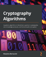
Suppose that we have a group of photons traveling all in the same direction on a predetermined axis. Moving in space, a photon has a vibration known as the polarization of the photon. The following diagram shows what we are talking about:

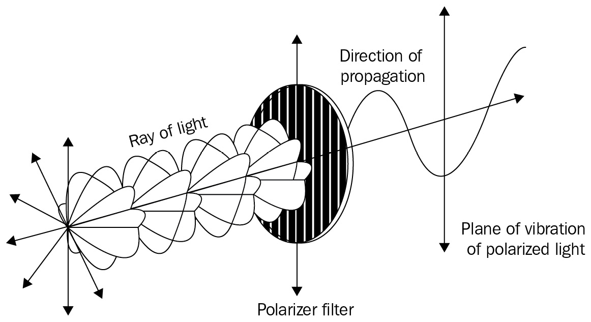
Figure 8.7 — Photon polarization

As you can see, photons spin their polarization in all directions. Still, if we place a filter, called a polaroid, oriented vertically, we will see that photons oriented vertically will pass across the filter 100% of the time. However, most of the other photons oriented in all directions will be blocked by the filter. In particular, the filter will block photons polarized perpendicularly to the filter 100% of the time, while photons oriented diagonally concerning the filter will pass (randomly) about 50% of the time. Moreover, these photons have to face a quantum dilemma: passing through the filter, they have to be observed, so they have to decide on their direction, deciding whether they want to assume a vertical orientation or a horizontal one.

This ability to block part of the photons is also explained in the experiment of polarized lenses. As shown in the following diagram, it's weird that if you add one more lens to the two already there, you can see much more light than before (see Polarizer 3):

Figure 8.8 – The polarized filter experiment

The result of this experiment on the polarized filter shows the preculiarity of the Q-Mechanics world; otherwise, our logic would lead us to think that less light can pass through by adding one more lens and that it should ideally get darker.

So, what Wiesner proposed was to create a special banknote in which there are 20 light traps. These traps are oriented in four directions, as shown in the following diagram of a 1-dollar note. The filters can detect (by combining themselves with the serial number on the note) whether the money is real or fake:

Figure 8.9 – Quantum 1-dollar banknote proposed by Wiesner

Only the bank that issues the notes can detect whether they are real or fake. In fact, due to the properties of Q-Mechanics, and in particular because of the indetermination principle, if someone wanted to counterfeit a note, it would be impossible to do so.

Let's see why an attacker would find it very hard to counterfeit one of these banknotes. In the preceding diagram, you can see the direction of the trap lights' orientation, but in reality, they are invisible so that nobody can see their orientation. Suppose Eve wants to copy the note; she can copy the serial number on the counterfeited note and try to figure out the traps' orientations.

If Eve decides to use a vertical filer to detect the polarization, she can detect all the vertical photons, and conversely, she will be sure that if the photon is horizontal, it will be blocked. But what about the others? Some of them will pass, but she will not be able to know exactly what polarization they have. So, the only thing Eve can do is randomly decide the polarization of all the photons so that they're different from the vertical and horizontal positions.

But now a problem occurs: if the bank runs a test on the banknote, they will know that it's fake. Because of the indetermination principle, only the bank knows the corresponding filter that's been selected for a determinate serial number.

Wiesner was always ignored when he talked about his invention of quantum money. It isn't a practicable invention to implement because the cost to set up such a banknote would be prohibitive; but this description introduces our next exploration well, which is the quantum key exchange.

Before we move on, just a note about quantum money: in his invention, Weisner intended to give banks the power to detect whether Eve had effectively attempted to counterfeit the note, but this concept is wrong. In fact, in the real world, the issue is not concerning banks (just a small part of the problem of counterfeit money affects banks). It is much more important that peer-to-peer users have control over judging the authenticity of banknotes. So, in my opinion, if quantum money ever comes out, it will be implemented in another way.

In the end, Wiesner found someone who listened to him, an old friend who was involved in different research projects and extremely curious about science: Charles Bennett. Charles spoke with Gilles Brassard, a researcher at the time in computer science at Montreal University; they started taking an interest in the problem and found out how to implement QKD, which we will explore next.

Quantum key distribution – BB84

Let's introduce BB84, the acronym that's Charles Bennett and Gilles Brassard developed in 1984 valid for QKD.

Now that we have learned about the properties of Q-Mechanics, we can use them to describe a technique for distributing bits (or better, quantum bits) through a quantum channel.

To describe what a quantum bit, also known as a qubit, is, we have to refer to the "quantum unit information" that's carried by qubits. Like traditional bits, (0) and (1), qubits are mathematical entities subject to calculation and operations.

We will use a bi-dimensional vectorial complex space of unitary length to define a qubit. So, we can say that a qubit is a unitary vector acting inside of a two-dimensional space. So far, we can think of a qubit as a polarized photon, similar to the entanglement experiment we looked at in the previous section. I have already introduced the notation to represent the qubits inside "bra-ket": |0> and |1>.

I will not go too deep into the mathematics of Q-Mechanics, but we have to go a bit deeper to analyze some of the properties of qubits.

If an element carries some information (like qubits do), it is related to a form of computational process, which in this case is quantum computing. We will return to this concept later when we talk about quantum computers. To understand the geometrical representation of a qubit, take a look at the following diagram:

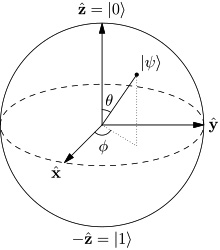
Figure 8.10 – Block sphere – the fundamental representation of a qubit

The difference between the classical computation we've used so far for all the classical bit operations, based on a Turing machine and Lambda calculus, and quantum computing is substantial. Quantum computing (related to computing with qubits) relies on superposition and entanglement properties. Qubits, as you saw when we discussed superposition, can be represented in a simultaneous state of (0) and (1), different from the normal bit, which can be only (0) or (1). We can mathematically represent qubits in the following way:

Figure 8.11 – Qubits represented in a mathematical way

Hence, considering a qubit as a unitary vector, it can be represented (as shown in the preceding diagram) as follows:

|ψ> = a |0> + b |1>  

Here, |a| and |b| are complex numbers, so the following applies:

|a| + |b| = 1

In other words, we only know that the value of the sum is (1), but we never know how a photon will be in a superposition state, so the values of the |a| and |b| coefficients are unpredictable.

For our scope, that is enough for us to explain the algorithm behind a quantum distribution key.

Now that we've provided a brief introduction to the basic concepts of quantum calculus and qubit operations, we are ready to explore the quantum transmission key algorithm.

Step 1 – Initializing the quantum channel

Alice and Bob need a quantum channel and a classical channel to exchange a message. The quantum channel is a channel where it is possible to send photons through it. Its characteristic is that it must be protected from the external environment. Any correlation with the external world has to be avoided. As we have seen, an isolated environment is necessary for achieving the superposition and entanglement of a particle.

The classical channel is a normal internet or telephonic line where Alice and Bob can exchange messages in the public domain.

We suppose that Eve (the attacker) can eavesdrop on the classical channel and can send and detect photons, just like Alice and Bob can.

Since the interesting part of the system is just the quantum channel, where Alice and Bob exchange the key, we are going to observe what happens in this channel because this is the real innovation of this system. Then, we will make some considerations about transmitting the message through the classical channel.

Step 2 – Transmitting the photons

Alice starts to transmit a series of bits to Bob. These bits are codified using a base that's randomly chosen for each bit while following these rules.

There are two possible bases for each bit:

B1 = {|↑>, |→>}  

and

B2 = {|↖>, |↗>}

If Alice choses B1, she encodes the following:

B1:    0 = |↑> and 1 = |→>

While if Alice chooses B2, then she will encode the following:

B2:    0 = |↖> and 1 = |↗>

Each time Alice transmits a photon, Bob chooses to randomly measure it with the B1 or B2 base. So, for each photon that's received from Alice, Bob will note the correspondent bit, (0) or (1), related to the base of the measurement that was used.

After Bob completes the measurements, he keeps them a secret. Then, he communicates with Alice through a classical channel and provides the bases (B1 or B2) that were used for measuring each photon, but not their polarization.

Step 3 – Determining the shared key

After Bob's communication, Alice responds, indicating the correct bases for measuring the photon's polarization. Alice and Bob only keep the bits that they have chosen the same bases for and discard all the others. Since there are only two possible bases, B1 and B2, Alice and Bob will choose the same base for about half of the bits that are transmitted. These bits can be used to formulate the shared key.

A numerical example is as follows.

Suppose that Alice wants to transmit the following bits sequence:

[0, 1, 1, 1, 0, 0, 1, 1]

Remember that the polarizations for each base are as follows:

B1:    0 = |↑> and 1 = |→>

B2:    0 = |↖> and 1 = |↗>

Alice randomly selects the bases:

• Alice's bases are B1, B2, B1, B1, B2, B2, B1, and B2.
• Alice's sequence is 0, 1, 1, 1, 0, 0, 1, 1.
• Alice's polarization is |↑>, |↗>, |→>, |→>, |↖>, |↖>, |→>, |↗>.
• Bob's choice is B2, B2, B2, B1, B2, B1, B1, and B2.
• Bob measurement is |↖>, |↗>, |↖>, |→>, |↖>, |↑>, |→>, |↗>.
• The correct bases are - |↗>, - |→>, |↖>, - |→>, |↗>.
• The corresponding bits are - 1 - 1, 0 - 1 1.
• So, the shared key is just the sequence of the selected bits [1, 1, 0, 1, 1].

The following is a representation of this scheme:

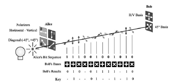
Figure 8.12 – Representation of QKD

At this point, we only need to check whether the two keys (from Alice and Bob) are identical.

Alice and Bob don't have to check the entire sequence but just a part of it to perform the parity bit control. If they check the entire parity sequence via the classical channel, it is obvious that Eve can spy on the conversation and steal the key. Therefore, they will decide to control only part of the sequence of bits.

Let's say that the key is of the order of 1,100 digits; they will check only 10% of the bits. After the parity control (made by a specific algorithm), they will discard the 100 bits that were processed in control and will keep all the others. This method lets them know that there were no errors in the transmission and detection process and whether Eve has attempted to observe the transmission in the quantum channel. The reason for this is related to Q-Mechanics' impossibility to observe a photon without forcing it to assume a direction of polarization (the indetermination principle). But if Eve measures the photons before Bob and allows the photons to continue for Bob's measurement, she will fail about half of the time. But when the same photon that's being measured by Eve arrives at Bob, he will have only a 25% probability of measuring an incorrect value. Hence, any attempt to intercept augments the error rating. That is why, after the third step, Alice and Bob performing parity control on the errors can also detect Eve's spying.

Now, the question of the millennium: is it possible for Eve to recover the key?

In other words, is this algorithm unbreakable?

Let's try to discover the answer in the next section, where we will analyze the possible attacks.

Analysis attack and technical issues

When we first described this algorithm, the assumption was that Eve has the same computational power as Bob and Alice and can spy on the conversations between them.

So, if Eve has a quantum computer in her hands and all the instruments to detect the photons' polarization, could she break the algorithm?

Let's see what Eve can do with her incommensurable computational power and the possibility of eavesdropping on the classical and quantum channels.

It looks like she is in the same situation as Bob (receiving photons). When Alice transmits the photons to Bob, even if the transmission comes through a quantum channel, if someone can capture the entire sequence of bits before Bob's selection, it's supposed that they will be able to collect the bits of the key. This could be true if Eve gets 100% of the measurements correct, but that is unthinkable for a key with a 1,000-bit length or more. Moreover, the attack will be discovered by Alice and Bob, as we will see now.

Let's analyze what can happen. Suppose that Alice transmits a photon with a polarization of |→> and Bob uses a base (B1) that's the same as Alice's. If Eve measures the photon with the same base (B1), the measurement will not alter the polarization, and Bob will correctly measure the photon's state. But if Eve uses B2, then she will measure the two states, |↖>, |↗>, with an equal probability. The photon that will arrive at Bob will only have half the probability of being detected as |→> and correctly measured. Considering the two possible choices Eve has to determine a correct or incorrect measurement, Bob will only have a 25% chance of measuring a correct value.

In other words, each time Eve attempts to measure augments the probability of an error rating occurring in Alice and Bob's communication. Therefore, when Alice and Bob go to check on the parity bits, they will identify the error and understand that an attack is being attempted. In this case, Alice and Bob will repeat the procedure, (hopefully) avoiding the attack again.

While analyzing the system, I endorse the thesis that this system is theoretically invulnerable, but I also agree that it is only a partial solution, mainly because this is not a quantum transmission message, but a quantum exchanging key. The reason I said it's theoretically invulnerable is that Eve can be detected by Bob and Alice by relying on the indetermination principle of Heisenberg. However, a man-in-the-middle attack, even if it doesn't arrive to recover the key (Eve can attempt to substitute herself with Bob), can block the key being exchanged between Alice and Bob, inducing them to repeat the operation infinite times.

In a document from the NSA, the National Security Agency of the United States, you can read about some weaknesses related to QKD and why it is discouraged that you implement it: https://www.nsa.gov/Cybersecurity/Quantum-Key-Distribution-QKD-and-Quantum-Cryptography-QC/.

What is to be understood is whether the NSA's concerns are related to the real possibility of implementing such a system or the possibility that hackers and other bad people could take advantage of this strong system.

In the NSA's document, we note some issues related to the implementation of QKD in a real environment. The NSA's notes are explained as follows:

• QKD is only a partial solution: The assumption is that the protocol doesn't provide authentication between the two actors. Therefore, it should need asymmetric encryption to identify Alice and Bob (that is, a digital signature) by canceling quantum security benefits. This problem could be avoided by using a quantum algorithm of authentication for implementing a quantum digital signature, if possible. Unfortunately, with the current state of the art, the way of identifying through a quantum algorithm and the non-repudiation of the message gives only a probabilistic result, far from the deterministic digital signature of the classical algorithms. Another solution is using a MAC (a function for authenticating symmetric algorithms), but again, it may not be quantum-resistant in the future.
• Costs and special equipment: This problem is concerned with higher costs and implementation problems for users. Moreover, the system is difficult to integrate with the existing network equipment.
• Security and validation: The issues, in this case, are related to the hardware being adapted to implement a quantum system. The specific and sophisticated hardware that's used for QKD can be subject to vulnerabilities.
• Risk of denial of service: This is probably the biggest concern of QKD. As I mentioned previously, Eve can repeat the attack on the quantum channel, sequentially causing Alice and Bob to never be able to determine a shared key.

As we have seen, the QKD method is not unerring. There is a remote possibility that someone, in practice, can break the system.

Note

QKD is just a part of the cryptographic transmission algorithm; the second part of the system is the encryption algorithm that's used to send the message, [M].

This is a fundamental part of Q-Cryptography's evolution because to be complete, the system should guarantee the transmission of the message, [M], through a quantum channel, but that needs another quantum algorithm. Moreover, the quantum authentication protocol remains unsolved.

We can say that QKD could be compared to Diffie–Hellmann, as RSA could be compared to a quantum message system transmission.

There are various choices we can make when it comes to transmitting messages in classical cryptography; we can use Vernam (as we saw in Chapter 1, Deep Diving into the Cryptography Landscape), which, combined with a random key (QKD), is theoretically secure, or another symmetric algorithm. But again, we don't rely on a fully quantum-based encryption system, which is autonomous and independent of classical mathematic problems.

Returning to the QKD algorithm, we have to find out why this algorithm is theoretically impossible to break, even with a quantum computer.

If an attacker decrypted a key generated with Q-Cryptography, the result of this action would probably be devastating for the entirety of Q-Mechanics. This is because one of the axioms that Q-Mechanics bases its strength on will be inconsistent: we are talking about the indetermination principle. If something like this happens, then the complete structure of Q-Mechanics would probably be involved in a revision process that would shock the pillars of the theory and all its corresponding physical and philosophical implications.

To establish this concept, I propose a theory: suppose that, in the future, someone will discover that the photons passing between the point of Alice's transmission and the point of Bob's measurement are truly random, but they follow a pre-determinate scheme. Suppose that this scheme is π or a Fibonacci series. In this case, the bits are effectively random, but their randomicity will be known so that Eve can forecast what the polarized scheme to adopt is.

What happens, for example, if we recognize that a sequence of digits such as "1415" is included in π?

As shown in the following code, π is a sequence composed of an infinite number of digits that follow the number 3, starting with "1415".... after the decimal point:

π = 3.14159265358979323846264338327950288419716939937510582097494459230781640628620899862803482534211706798214808651328230664709384460955058223172535940812848111745028410270193852110555964462294895493038196442881097566593344612847564823378678316527120190…

We can go on following the π sequence and recovering all the other digits after 1415 that are: 92653589...

Undoubtedly, I agree with the NSA's report when they said that QKD is an incomplete algorithm. It misses the second part of the algorithm, which completes the encryption of the message: [M] into the quantum channel. By using BB84, this stage is devolved to classical cryptography because after exchanging the key (in the quantum channel), we must encrypt the message using a classic encryption algorithm.

As I have always been against hybrid schemes, I have projected that a quantum encryption algorithm would be valid for quantum message system transmission. Its name is QMB21, and it will hopefully become a standard for the next Q-Cryptography transmissions. Due to issues linked to the process of patenting, it is not possible to explain the algorithm here. I hope to be able to update this section with more details on this innovation soon.

Now that we have analyzed the Q-Cryptography key distribution, another challenge awaits: exploring quantum computing and what it will be able to do when its power increases.

Quantum computing

In this section, I will talk about quantum computing and quantum computers. The difference between the two is that quantum computing is the computational power that's expressed by a quantum system, while a quantum computer is the system's physical implementation, which is composed of hardware and software. The first idea of a quantum computer was originally proposed by Richard Feynman in 1982; then, in 1985, David Deutsch formulated the first theoretical model of it. This field had a big evolution in the last decades; some private companies began to take action and experiment with new models of quantum computers. Some of them, such as D-Waves and Righetti Computing, raised millions of dollars for the research and development of these machines and their relative software:

Figure 8.13 – D-Waves quantum computer

As you should already know, normal computers work with bits, while quantum computers work with qubits. As we have also already seen, a qubit has a particular characteristic in that it can be simultaneously in the state of (0) and (1). Just this information by itself suggests a greater capability of computation concerning a normal computer.

A normal computer works by performing each operation one by one until it reaches the result. Conversely, a quantum computer can perform more operations at the same time. Moreover, many qubits can be linked together in a state of entanglement. This phenomenon creates a new state of superposition over the multiple combinations of the entangled qubits, elevating the grade of computation of a quantum computer exponentially compared to a normal one. So, we are not only talking about a parallelization process of computation but also an exponential computation process when augmenting the number of qubits in the game. Therefore, to give you an idea of the computational power that's created by a quantum computer, n qubits can generate a capability to elaborate information 2^n times compared to classical bits.

Let's consider the preceding sentence. In a state of superposition or entanglement, 8 qubits, for instance, can represent any number between 0 and 255 simultaneously. This is because 2^8 = 256, so we have 256 possible configurations each time, which, expressed in binary notation, looks like this:

0 = (0)2 —————> 255 = (11111111)2

We can understand the supremacy of a quantum computer, especially if we deal with two specific problems of extreme interest to cryptography: the factorization problem and searching on big data.

These two arguments are considered very hard to solve for a classical computer; we have seen, for instance, the RSA algorithm and other cryptographic algorithms relying on factorization to generate a one-way function that's able to determine a secured cryptogram. However, the community's recurring question is, how long will classical cryptography resist when a quantum computer reaches enough qubits to perform operations that are considered unthinkable?

We will try to answer this question after exploring the potential of a quantum computer and seeing what we can do with one by projecting one adapted for our scopes.

As we mentioned previously, a quantum computer can simultaneously perform all the state bases of a linear combination. Effectively, in this sense, a quantum computer can be considered an enormous parallel machine that's able to calculate huge states of combinations in parallel.

For example, to understand what a quantum computer can do, let's take three particles: the first of orientation 1 and the last two with an orientation of 0 (relative to some base). We can represent this as follows:

|100>  

The quantum computer can take |100> as input and give some output, but at the same time, it could take a normalized combination of the three particles (of length = 1) with a state base as input, as follows:

1/√3(|100>  + |100>  + |100>)

As a result, it gives an output in only one operation as it computes only the state base.

After all, the quantum computer doesn't know whether a photon is in one state base or multiple combinations of states until a measurement occurs (the indetermination principle).

This ability to elaborate combinations of linear states simultaneously determines the quantum supremacy of quantum computers.

So, while a classical computer (even the most powerful supercomputer on the earth) requires a string of bits as input and returns a string of bits as output (even if it's parallelizing billions of operations), it will not be able to perform a function that accepts the following sum as input:

1/C ∑ |x>

Here, C is a normalization factor of all the possible states of the input. The function would return the following as output:

1/C ∑ |x,f(x)>

Here, |x,f(x)> is a succession of bits longer than |x|, which represents both |x| and f(x).

To understand this concept, you can think of having a sum of bits, (C), and in this sum, all the possible states of (m) qubits in a superposition are hidden. So, we can say that (C) represents the number of all the states that the qubits are in at the same time.

You can imagine how fantastic that could be! But still, there is a problem: the measurement. We have seen that when we measure the quantum computation, this measurement freezes the qubits in only one state, which is governed by randomness. Therefore, we can force the system to appear in a state, as follows:

|x0,f(x0)>

This is for some x0 value that's randomly chosen, so all the other states are going to be destroyed.

In this case, the ability to program a quantum computer makes it possible to create a quantum computation that provides a very high-probability result of getting the desired output.

To understand the process of implementing a quantum algorithm, let's look at a candidate algorithm that could wipe out a great part of classical cryptography: Shor's algorithm.

Shor's algorithm

In a recent interview with David Deutsch (considered one of the fathers of quantum computing), the interviewer posed a question about the philosophy of superposition, asking David, "In what way does the Quantum Computing community give credit to the hypothesis of a multiverse?"

David's answer refers to Q-Cryptography and, in particular, he tries to demonstrate the existence of the multiverse through the factorization problem. I will try to paraphrase David's answer in the following paragraph:

Imagine deciding to factorize an integer number of 10,000 digits, a product of two big prime numbers. No classical computer can express this number as the product of its prime factors. Even if we take all the matter contained in the universe and transform it into a supercomputer, which starts to work for a time long, such as the universe's time, this instrument will not be able to scratch the surface of the factorization problem. Instead, a quantum computer should be able to solve this problem in a few minutes or seconds. How is this possible?

Whoever is not a solipsist has to admit that the answer is linked to some physics process. We know that not enough power exists in the universe to calculate and obtain an answer, so something has to happen compared to what we can see directly. At this point, we have already accepted the structure of the multiverse (otherwise known as superposition).

The way (described by Deutsch) in which a quantum computer works is as follows:

"The universe has evolved into multiple universes and in each, different sub-calculation is performed. The number of sub-calculations is enormously bigger than all the atoms contained in the known universe. In the end, the results became englobed to obtain a unique answer. Whoever neglects the existence of multiverses has to explain how the factorization process works."

After this interesting digression into quantum computational power, let's dive deeper and analyze Shor's algorithm mathematically and logically; this algorithm is the true representation of what happens in a quantum computer at work.

The hypothesis, by Fermat's Last Theorem, is as follows: say you find two (non-trivial) values, (a) and (r), so the following applies:

a^r ≡ 1 (mod n)

Here, there is a good possibility of factorizing (n).

We start to randomly choose a number, (a), and consider the following sequence of numbers:

1, a, a^2, a^3, … , a^n (mod n)

The thesis is that we can find a period for this sequence that we call (r), which will be repeated every (r) time when we elevate (a) to (r) so that we will have solved the following equation for (r), which always gives (1) as a result:

a^r ≡ 1 (mod n)

Therefore, we want to program our quantum computer to find an output, (r), to be able to factorize (n) with a high probability.

Step 1 – Initializing the qubits

We choose a number, (m), so that the following applies:

n^2 ≤ 2^m < 2^n

Supposing we choose m = 9, this means that we have 9 bits initialized with their state all in (0), and we mathematically represent it as follows:

m = 9 : |000000000>

Changing the axes of the bits, we can transform the first bit into a linear combination of |0> and |1>, which gives us the following:

1/√ 2  (|000000000> + |100000000>)   

By performing a similar transformation on every single bit of (m) inside bra-ket until the m-bit to obtain the quantum state, we get a sequence like this:

1/√ 2^m (|000000000> + |000000001>+ |000000010> + . . . + |111111111>)

Remember that m = 9, so 2^m = 512; we will have 512 multiple combinations of bits, given by the first, |000000000 = 0, and the last, |2^m-1> = |111111111> = 511 (in decimal notation).

In a sum like this, all the possible states of the m qubits are overlying in a superposition. Now, for simplicity regarding notation, we will rewrite the m qubits in cardinal numbers:

1/√ 2^m (|0> + |1>+ |2>+ . . . + |2^m-1>)

The preceding functions are just the same as the previous ones but are represented in cardinal numbers.

Step 2 – Choosing the random number, a

Now, we must choose a random number (a) so that the following applies:

1 < a < n

Quantum computing computes the following function:

fx ≡ a^x (mod n)

It returns the following:

1/√ m^2 (|0, a^0 (mod n)> + |1, a^1 (mod n)>+ |2, a^2 (mod n)>+ . . . + |2^m-1, a^2m-1 (mod n)>)

When visualizing this function, you can lose the sense of representation because it appears rather complex; so, to simplify it, forget the modulus, n, that's repeated for each operation and rewrite the previous functions like so:

1/√ m^2 (|0, a^0 > + |1, a^1 >+ |2, a^2>+ . . . + |2^m-1, a^2m-1>)

Again, consider that all the operations are in (mod n), but focus on the sense of the functions: it says that we have to elevate (a) to all the (2^m-1) states of the m qubits.

However, so far, the state of this representation doesn't provide any more information compared to a classical computer.

Now, it's time to look at an example to help you understand what we are doing.

Suppose that n = 21 (a very easy number to factorize); however, the size of the number is not important now but the method is.

Here, we choose randomly a = 11.

So, we calculate the values of 11^x (mod 21) that have been transposed into the function:

1/√ 512 (|0, 1> + |1, 11> + |2, 16> + |3, 8> + |4, 4> + |5, 2> + |6, 1> + |7, 11> +

|8, 16> + |9, 8> + |10, 4> + |11, 2> + |12, 1> + |13, 11> + |14, 16> + |15, 8> +

|16, 4> + |17, 2>. . . . . . . . . . . .+ |508, 4> + |509, 2> + |510, 1> + |511, 11>)

As you can see, this is a development of the entire sequence, where 1/√ 512 = 1/ C and C is the number of states of m = 2^9.

Each qubit is composed of a sequence number, (a^x (mod 21)). Take the following example:

|1, 11> ≡ 11^1  (mod 21) = 11

Step 3 – Quantum measurement

If we measure only the second part of the sequence, a^x, then the function collapses in a state that we cannot control. However, this measurement is the essence of the system. In fact, because of this measurement, the entire sequence collapses for some random base, (x0), so the following applies:

|x0, a^x0>

Now, it should be clearer to you that we can force the system to appear in a state, as follows:

|x0, f(x0)>

So, after the measurement, the state of the system is fixed (in other words, a number appears) in only one base (x0) that we suppose to be as follows:

x0 = 2

Forgetting all the other values of a^x (that we have previously calculated) and picking up only the ones that have a value equal to 2, we will extract the following highlighted values:

1/√ 512 (|0, 1> + |1, 11> + |2, 16> + |3, 8> + |4, 4> + |5, 2> + |6, 1> + |7, 11> +

|8, 16> + |9, 8> + |10, 4> + |11, 2> + |12, 1> + |13, 11> + |14, 16> + |15, 8> +

|16, 4> + |17, 2>. . . . . . . . . . . .+ |508, 4> + |509, 2> + |510, 1> + |511, 11>)

To simplify the notation, we must discard the second part of the qubit (2) because it is superfluous:

1/√ 85 (|5> + |11> + |17>. . . . . . .+ |509>)

Here, 85 stands for the number of m qubits selected.

Now, if we make a measurement, we will find a value, x, so that the following applies:

11^x ≡ 2 (mod 21)

Unfortunately, this information is not useful for us. But don't lose hope.

Step 4 – Finding the right candidate, (r)

Recall that we have programmed our quantum computer with a specific scope: to find the output in the system that can factorize (n). To reach our goal, we have to find the value of (r) so that the following applies:

a^r ≡ 1 (mod n)

Generally, when we deal with functions such as a^x (mod n), we know that the values of (x) are periodic, with a period of (r) where a^r = 1 (mod n).

So, recalling the previous function in which the selected elements appear, we have the following:

|5> + |11> + |17>. . . . . .+ |509>

As you can see, the period is r = 6.

Therefore, we can verify whether the following applies:

11^r ≡ 1 (mod 21)

11^6 ≡ 1 (mod 21)

Here we go!

Hence, r = 6 is a very good candidate for us.

Note

In this example, we can see that r = 6 is the period of the function, though it's not always easy to work out. There is a mathematical way to discover the period of a function. Using the Quantum Fourier Transform (QFT), we can discover the period (if it exists). If you want to continue looking at the demonstration of Shor's algorithm, you can skip the next section and go directly to the last step of Shor's, coming back to QFT on your second read.

Quantum Fourier Transform

Let's discover a little bit more about the Fourier Transform (FT) and QFT.

FT is a mathematical function. It can be intuitively thought of like a musical chord in terms of volume and frequency. The FT can transform an original function into another function, representing the amount of frequency present in the original function. The FT depends on the spatial or temporal frequency and is referred to as a time domain. It is represented by a graphic that shows the frequency that was detected, as shown in the following diagram:

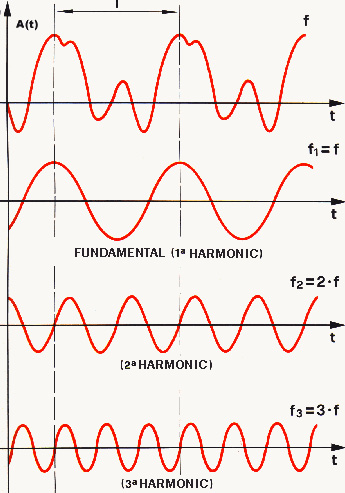
Figure 8.14 – Fourier Transform

To understand how this works, let's look at an example of FT taking an arithmetic succession of numbers, like so:

1, 3, 7, 2, 1, 3, 7, 2

As you can see, we have the first four numbers – 1, 3, 7, 2 – which get repeated two times. In other words, we can break the succession into two parts:

1,3,7,2 | 1,3,7,2

Note

The | symbol represents, in this case, splitting the succession into two parts.

Here, we can say that this succession has a length of 8 and a period of 4. The length, divided by the period, gives us the frequency (f):

f = 8/4 = 2

In this case, f = 2 is the number of times that the succession is repeated.

Now, we can enounce the general rule of FT. Suppose we have a succession that's 2^m in length for any integer, m:

[a0, a1, ...., a2^m-1]

We can define the FT with the following formula:




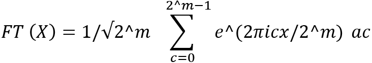
We can define the following part of the formula with j:

j = e ^ (2πicx/2^m)

The x parameter runs in the following range:

0 ≤ x < 2^m

With the FT formula, you can find the frequency of the succession while using determinate parameters as input. If we suppose, for example, cx = 1 and m = 3, then we have the following substitution:

j = e^(2πi/8)

By substituting the different values of x in the equation with j, we obtain the following result by exploding the formula for FT(1):

√ 8 FT(1) = 1+ 3j + 7j^2 + 2j^3 + j^4 + 3j^5 + 7j^6 + 2j^7 = 0

Since all the terms of the succession get eliminated, we have the following:

• FT(X0) with x = 0 ---> e^0 = 1, which is the result of FT(X0) = 1
• FT(X4) with x = 4 ---> e^πi = -1, which is the result of FT(X4) = -1

So long as j^4 = -1, all the terms will be deleted and we will obtain FT(1) = 0.

Instead, for FT(0), the result of the numerator addition corresponds to the sum of all the terms of the sequence:

1 + 3 + 7… + 2 = 26

Continuing, we have the following:

FT(0) = 26/√ 8                  FT(2) = (-12 +2i) /√ 8

FT(4) = 6/√ 8                   FT(6) = (-12 -2i) /√ 8

For all the other terms, FT(1) = FT(3) = FT(5) = FT(7) = 0.

In other words, the FT confirms what we have deducted since the beginning of this example – that is, in the succession 1, 3, 7, 2, 1, 3, 7, 2, the peaks of the function correspond with the non-zero values of (FT) that are multiples of 2: the frequency.

This result will be very useful in Shor's algorithm to discover the period of the function, as we will see shortly.

But we want to program our algorithm in a quantum computer, so we need a version of FT that's been adapted for quantum algorithms.

QFT is what we need to detect the frequencies that we use to find the period (r) in Shor's algorithm. It is defined on a base state of |X⟩ with (or ≤ x <2^m):




As you can see, the FT (shown previously in this chapter) and QFT (shown here) are very similar. The difference is that QFT is acting in a quantum environment, so the c parameter of FT now appears in a quantum state, |c⟩, and the same is valid for |X⟩.

Returning to our quantistic example of Shor's algorithm, we can apply the QFT to it to discover the frequency:

QFT (1/√ 85 (|5> + |11> + |17>. . . . . . .+ |509>))

We obtain the following sum:

1/√85 ∑ g(c) |c⟩

For c, this runs from 0 to 511. Here:




This is the FT of the following succession:

0,0,0,0,0,1,0,0,0,0,0,1..... 0,0,0,0,0,1,0,0

By applying a break symbol to the succession, we can visualize the frequency:

0,0,0,0,0,1 |0,0,0,0,0,1 |..... 0,0,0,0,0,1 |,0,0

As you can see, the frequency of this succession is around 512/6 ~ 85.

In this sinusoidal function, which is given by waves in which there are high and low points, the picks (highest points of interest) of the function correspond with the following:

c = 0, 85, 171, 256, 314, 427

We expect that 427 is a multiple of the frequency we are looking for:

427 ~ j f0  

This applies so long as the following is true:

427/512 ~ 5/6

So, we expect that r = 6 is the period.

Note

I didn't show all the mathematical passages that bring us to the result of r = 6, but the intention is to give you a demo of the possibility to apply QFT to this algorithm. For a deeper analysis of QFT, go to the following learn session of the IBM Quantum Lab project: https://qiskit.org/textbook/ch-algorithms/quantum-fourier-transform.html.

Now that we know what QFT does and how to use it in Shor's algorithm, let's perform factorization through a quantum algorithm.

Step 5 – Factorizing (n)

The last step of Shor's algorithm uses the greatest common divisor (GCD) to calculate whether the candidate (r) gives back the two factors of (n).

As you probably remember from high school, the GCD is the greatest positive common divisor between two numbers. It can also be used to reduce a fraction to its smallest possible divisors.

Regarding the Mathematica software, there's a very useful reduction function that is implemented when you divide by two integers.

In our case, if r = 6 and n = 21, we just divide the two numbers:

In[01]: = GCD[21, 6]

Out[01]: = 3

Here, I have told Mathematica to perform GCD[21,6], finding the number (3): the GCD between (21) and (6).

Now, by reducing the fraction (the operation consists of dividing both 21 and 6 by 3), we get 7 as the second output:

In[02]: = 21/6

Out[02]: = 7/2

Therefore, 21 = 7*3.

We got the solution!

Notes on Shor's algorithm

Peter Shor presented this algorithm when the quantum computer hadn't been experimented with and built up in practice. Here, I provided an example of how it could be possible to perform a factorization in a theoretical way on a quantum computer, but at the moment, no machine exists that can perform this algorithm in a scalable way.

Moreover, Shor's algorithm is not deterministic. Still, it gives a probabilistic grade to find the factors, even if, generally, after a few steps (if the first candidate that's found is discarded), it will be possible to find a good candidate for the factorization of (n).

From the opposite point of view, if a scalable quantum computer were to be implemented and ready to run this algorithm in the future, it will probably be the end of classical cryptography.

But now, it's time to answer our initial question about quantum computers, reformulated appropriately: what are the consequences of cryptography when the quantum computer reaches enough qubits to perform Shor's algorithm?

Let's discuss this topic in the final section of this chapter, dedicated to post-Q-Cryptography.

Post-Q-Cryptography

It is useful to point out that post-Q-Cryptography has nothing to do with Q-Cryptography, except for the fact that it could be considered resistant to quantum computing (maybe it is only a chimera). When we talk about post-Q-Cryptography, we refer to classical algorithm candidates being resistant to quantum computing.

If quantum computing were to raise its power, expressed in a satisfying number of qubits, and were implemented on appropriate hardware able to perform the quantum computation, many of the algorithms that have been discussed in this book would be breached. However, nowadays, a quantum computer occupies an entire room of space and works through hardware made by several components (most of them prepared to keep the qubits in a state of entanglement at frozen temperatures). As soon as the dimensions of the hardware are reduced and its calculation power increases, most of the following algorithms will probably fail in terms of timing, which could swing between 1 hour and a few days: RSA and Diffie–Hellman, Schnorr protocols, and most of the zero-knowledge protocols – even elliptic curves; it is supposed that most elliptic curves implementations will be breakable.

Based on a document provided by the European Commission for Cybersecurity (ENISA) released in February 2021, some categories of algorithms could support the shock wave of quantum power computation.

In this study, the commission commented on the advent of quantum computing:

"It is thus important to have replacements in place well in advance. What makes matters worse is that any encrypted communication intercepted today can be decrypted by the attacker as soon as he has access to a large quantum computer, whether in 5, 10, or 20 years from now; an attack known as retrospective decryption."

The categories of algorithms that are reputed to be resilient to quantum computing, many of them previously evaluated by NIST, are as follows:

• AES: This is considered a good post-quantum candidate: we saw this algorithm in Chapter 3, Asymmetric Encryption.
• Hash functions: We saw these functions in Chapter 4, Introducing Hash Functions and Digital Signatures.
• Code-based cryptography: This uses the technique of error-correction code, based on a proposal by McEliece.
• Isogeny-based cryptography: This is a kind of cryptography based on adding points to elliptic curves over finite fields.
• Lattice-based cryptography: Among these algorithms, the NTRU algorithm is probably one of the best candidates that resists quantum computing.

All these categories are supposed to be quantum-resistant, based on evaluations given on mathematics and cryptoanalysis of the mentioned systems. However, some skeptical thoughts are spreading among the community, most of which are often calmed down by announcements about minimizing problems.

Summary

In this chapter, we analyzed Q-Cryptography. After introducing the basic principles of Q-Mechanics and the fundamental bases of this branch of science, we deep-dived into QKD.

After that, we explored the potential of quantum computing and Shor's algorithm. This algorithm is a candidate for wiping out a great part of classical cryptography when it comes to implementing a quantum computer that will get enough qubits to boost its power against the factorization problem.

Finally, we saw the candidate algorithms for the so-called post-Q-Cryptography; among them, we saw AES, SHA (hash), and NTRU.

With that, you have learned what Q-Cryptography is and how it is implemented. You have also learned what quantum computing is and, in particular, became familiar with a very disruptive algorithm that you can implement in a quantum machine: Shor's algorithm.

Finally, you learned which algorithms are quantum-resistant to the power of the quantum computer and why.

These topics and the concepts that were explained in this chapter are essential because the future of cryptography will rely on them.

Now that you have learned about the fundamentals of Q-Cryptography and most of the principal cryptography algorithms that have been produced until now, it is time to move on to the next chapter, where we will look at the Crypto Search Engine. The next chapter will provide you with knowledge about search engine logic. Then, we will explore an innovative search engine platform that works with encrypted data, developed by my team and me.