I am dying to hear about it, since I always thought number theory was the Queen of Mathematics—the purest branch of mathematics—the one branch of mathematics which has NO applications!
Now that we are fitted out with a sturdy tool box of arithmetic functions that we developed in the previous chapters, we turn our attention to the implementation of several fundamental algorithms from the realm of number theory. The number-theoretic functions discussed in the following chapters form a collection that on the one hand exemplifies the application of the arithmetic of large numbers and on the other forms a useful foundation for more complex number-theoretic calculations and cryptographic applications. The resources provided here can be extended in a number of directions, so that for almost every type of application the necessary tools can be assembled with the demonstrated methods.
The algorithms on which the following implementations are based are drawn primarily from the publications [Cohe], [HKW], [Knut], [Kran], and [Rose], where as previously, we have placed particular value on efficiency and on as broad a range of application as possible.
The following sections contain the minimum of mathematical theory required to explicate the functions that we present and their possibilities for application. We would like, after all, to have some benefit from all the effort that will be required in dealing with this material. Those readers who are interested in a more thoroughgoing introduction to number theory are referred to the books [Bund] and [Rose]. In [Cohe] in particular the algorithmic aspects of number theory are considered and are treated clearly and concisely. An informative overview of applications of number theory is offered by [Schr], while cryptographic aspects of number theory are treated in [Kobl].
In this chapter we shall be concerned with, among other things, the calculation of the greatest common divisor and the least common multiple of large numbers, the multiplicative properties of residue class rings, the identification of quadratic residues and the calculation of square roots in residue class rings, the Chinese remainder theorem for solving systems of linear congruences, and the identification of prime numbers. We shall supplement the theoretical foundations of these topics with practical tips and explanations, and we shall develop several functions that embody a realization of the algorithms that we describe and make them usable in many practical applications.
That schoolchildren are taught to use the method of prime factorization rather than the more natural method of the Euclidean algorithm to compute the greatest common divisor of two integers is a disgrace to our system of education.
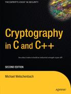
Stated in words, the greatest common divisor (gcd) of integers a and b is the positive divisor of a and b that is divisible by all common divisors of a and b. The greatest common divisor is thereby uniquely determined. In mathematical notation the greatest common divisor d of two integers a and b, not both zero, is defined as follows: d = gcd(a, b) if d > 0, d | a, d | b, and if for some integer d' we have d' | a and d' | b, then we also have d' | d.
It is convenient to extend the definition to include
| gcd(0,0) := 0. |
The greatest common divisor is thus defined for all pairs of integers, and in particular for the range of integers that can be represented by CLINT objects. The following rules hold:
of which, however, only (i)-(iii) are relevant for CLINT objects.
It is obligatory first to consider the classical procedure for calculating the greatest common divisor according to the Greek mathematician Euclid (third century B.c.E.), which Knuth respectfully calls the grandfather of all algorithms (definitely see [Knut], pages 316 ff.). The Euclidean algorithm consists in a sequence of divisions with remainder, beginning with the reduction of a mod b, then b mod (a mod b), and so on until the remainder vanishes.
Euclidean algorithm for calculating gcd(a, b) for a, b ≥ 0
If b = 0, output a and terminate the algorithm.
Set r ← a mod b, a ← b, b ← r, and go to step 1.
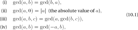
For natural numbers a1, a2 the calculation of the greatest common divisor according to the Euclidean algorithm goes as follows:
This procedure works very well for calculating the greatest common divisor or for letting a computer program do the work. The corresponding program is short, quick, and, due to its brevity, provides few opportunities for error.
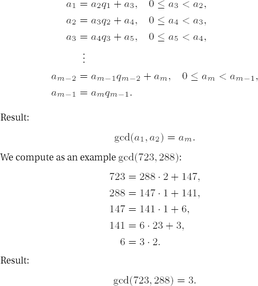
A consideration of the following properties of integers and of the greatest common divisor indicates—at least theoretically—possibilities for improvement for programming this procedure:
The advantage of the following algorithm based on these properties is that it uses only size comparisons, subtractions, and shifts of CLINT objects, operations that do not require a great deal of computational time and for which we use efficient functions; above all, we need no divisions. The binary Euclidean algorithm for calculating the greatest common divisor can be found in almost the identical form in [Knut], Section 4.5.2, Algorithm B, and in [Cohe], Section 1.3, Algorithm 1.3.5.
Binary Euclidean algorithm for calculating gcd(a, b) for a, b ≥ 0
If a < b, exchange the values of a and b. If b = 0, output a and terminate the algorithm. Otherwise, set k ← 0, and as long as a and b are both even, set k ← k + 1, a ← a/2, b ← b/2. (We have exhausted property (i); a and b are now no longer both even.)
As long as a is even, set repeatedly a ← a/2 until a is odd. Or else, if b is even, set repeatedly b ← b/2 until b is odd. (We have exhausted property (ii); a and b are now both odd.)
Set t ←(a - b)/2. If t = 0, output 2ka and terminate the algorithm. (We have used up properties (ii), (iii), and (iv).)
As long as t is even, set repeatedly t ← t/2, until t is odd. If t > 0, set a ← t; otherwise, set b ← -t; and go to step 3.
This algorithm can be translated step for step into a programmed function, where we take the suggestion from [Cohe] to execute in step 1 an additional division with remainder and set r ← a mod b, a ← b, and b ← r. We thereby equalize any size differences between the operands a and b that could have an adverse effect on the running time.
Function: | greatest common divisor |
Syntax: | |
Input: |
|
Output: |
|
void
gcd_l (CLINT aa_l, CLINT bb_l, CLINT cc_l)
{
  CLINT a_l, b_l, r_l, t_l;
  unsigned int k = 0;
  int sign_of_t;
Note
Step 1: If the arguments are unequal, the smaller argument is copied to b_l. If b_l is equal to 0, then a_l is output as the greatest common divisor.
if (LT_L (aa_l, bb_l))
  {
    cpy_l (a_l, bb_l);
    cpy_l (b_l, aa_l);
  }
else
  {
    cpy_l (a_l, aa_l);
    cpy_l (b_l, bb_l);
  }
if (EQZ_L (b_l))
  {
    cpy_l (cc_l, a_l);
    return;
  }
Note
The following division with remainder serves to scale the larger operand a_l. Then the powers of two are removed from a_1 and b_1.
(void) div_l (a_l, b_l, t_l, r_l);
cpy_l (a_l, b_l);
cpy_l (b_l, r_l);
if (EQZ_L (b_l))
  {
    cpy_l (cc_l, a_l);
    return;
  }
while (ISEVEN_L (a_l) && ISEVEN_L (b_l))
{
++k;
shr_l (a_l);
shr_l (b_l);
}Note
Step 2.
while (ISEVEN_L (a_l))
  {
    shr_l (a_l);
  }
while (ISEVEN_L (b_l))
  {
    shr_l (b_l);
  }
Note
Step 3: Here we have the case that the difference of a_l and b_l can be negative. This situation is caught by a comparison between a_l and b_l. The absolute value of the difference is stored in t_l, and the sign of the difference is stored in the integer variable sign_of_t. If t_l == 0. Then the algorithm is terminated.
do
  {
    if (GE_L (a_l, b_l))
      {
        sub_l (a_l, b_l, t_l);
        sign_of_t = 1;
      }
    else
      {
        sub_l (b_l, a_l, t_l);
        sign_of_t = −1;
      }
    if (EQZ_L (t_l))
      {
        cpy_l (cc_l, a_l);      /* cc_l <- a */
        shift_l (cc_l, (long int) k);        /* cc_l <- cc_l*2**k */
        return;
}while (ISEVEN_L (t_l))
{
shr_l (t_l);
}
if (-1 == sign_of_t)
{
cpy_l (b_l, t_l);
}
else
{
cpy_l (a_l, t_l);
}
}
while (1);
}Although the operations used are all linear in the number of digits of the operands, tests show that the simple two-line greatest common divisor on page 168 is hardly slower as a FLINT/C function than this variant. Somewhat surprised at this, we ascribe this situation, for lack of better explanation, to the efficiency of our division routine, as well as to the fact that the latter version of the algorithm requires a somewhat more complex structure.
The calculation of the greatest common divisor for more than two arguments can be carried out with multiple applications of the function gcd_l(), since as we showed above in (10.1)(iii) the general case can be reduced recursively to the case with two arguments:
With the help of the greatest common divisor it is easy to determine the least common multiple (lcm) of two CLINT objects a_l and b_l. The least common multiple of integers n1,...,nr, all nonzero, is defined as the smallest element of the set
We shall use this relation for the calculation of the least common multiple of a_l and b_l.
Syntax: | |
Input: |
|
Output: |
|
Return: |
|
int
lcm_l (CLINT a_l, CLINT b_l, CLINT c_l)
{
  CLINT g_l, junk_l;
  if (EQZ_L (a_l) || EQZ_L (b_l))
    {
      SETZERO_L (c_l);
      return E_CLINT_OK;
    }
  gcd_l (a_l, b_l, g_l);
  div_l (a_l, g_l, g_l, junk_l);
  return (mul_l (g_l, b_l, c_l));
}
It holds for the least common multiple as well that its calculation for more than two arguments can be recursively reduced to the case of two arguments:
Formula (10.4) above does not, however, hold for more than two numbers: The simple fact that lcm(2,2,2) • gcd(2,2,2) = 4 ≠ 23 can serve as a counterexample. There does exist, however, a generalization of this relation between the greatest common divisor and the least common multiple for more than two arguments. Namely, we have
and also
The special relationship between the greatest common divisor and the least common multiple is expressed in additional interesting formulas, demonstrating an underlying duality, in the sense that exchanging the roles of greatest common divisor and least common multiple does not affect the validity of the formula, just as in (10.6) and (10.7). We have the distributive law for gcd and lcm, namely,
and to top it all off we have (see [Schr], Section 2.4)
Aside from the obvious beauty of these formulas on account of their fearful symmetry, they also serve to provide excellent tests for functions that deal with greatest common divisor and least common multiple, where the arithmetic functions used are implicitly tested as well (on the subject of testing, see Chapter 12).
Don't blame testers for finding your bugs.
In contrast to the arithmetic of whole numbers, in residue class rings it is possible, under certain assumptions, to calculate with multiplicative inverses. Namely, many elements
The existence of multiplicative inverses in • n is not obvious. In Chapter 5, on page 69, it was determined only that (• n,.) is a finite commutative semigroup with unit
can be transformed into
If we continue in this fashion, then we obtain in succession
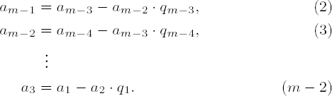
If in (1) we replace am-1 by the right side of equation (2), then we obtain
or
Proceeding thus one obtains in equation (m - 2) an expression for am as a linear combination of the starting values a1 and a2 with factors composed of the quotients qi of the Euclidean algorithm.
In this way we obtain a representation of gcd(a, b) = u • a + v • b =: g as a linear combination of a and b with integer factors u and v, where u modulo a/g and v modulo b/g are uniquely determined. If for an element
| 3 = 141 - 6 • 23, |
| 6 = 147 - 141 • 1, |
| 141 = 288 - 147 • 1, |
| 147 = 723 - 288 • 2. |
From this we obtain our representation of the greatest common divisor:
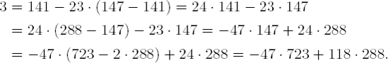
A fast procedure for calculating this representation of the greatest common divisor would consist in storing the quotients qi (as is done here on the page) so that they would be available for the backward calculation of the desired factors. Because of the high memory requirement, such a procedure would not be practicable. It is necessary to find a compromise between memory requirements and computational time, which is a typical tradeoff in the design and implementation of algorithms. To obtain a realistic procedure we shall further alter the Euclidean algorithm in such a way that the representation of the greatest common divisor as a linear combination can be calculated along with the greatest common divisor itself. For
associativity of (• n,.),
commutativity of (• n,.),
existence of a unit: For all

carry over directly to (• nx,•). The existence of multiplicative inverses holds because we have selected precisely those elements that have such inverses, so that we have now only to demonstrate closure, namely, that for two elements
The number of elements in •nx, or, equivalently, the number of integers relatively prime to n in the set {1,2,...,n - 1}, is given by the Euler phi function
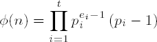
(see, for example, [Nive], Sections 2.1 and 2.4). This means, for example, that •
If gcd(a, n) = 1, then according to Euler's generalization of the little theorem of Fermat,[20] a
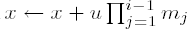
We do significantly better, namely with a computational cost of O (log2 n) and without knowing the value of the Euler phi function, by integrating the above constructive procedure into the Euclidean algorithm. For this we introduce variables u and v, with the help of which the invariants
are maintained in the individual steps of the procedure presented on page 169, in which we have
and these invariants provide us at the end of the algorithm the desired representation of the greatest common divisor as a linear combination of a and b. Such a procedure is called an extended Euclidean algorithm.
The following extension of the Euclidean algorithm is taken from [Cohe], Section 1.3, Algorithm 1.3.6. The variable v in the above invariant condition is employed only implicitly, and only at the end is it calculated as v := (d-u•a)/b.
Extended Euclidean algorithm for calculating gcd(a, b) and factors u and v such that gcd(a, b) = u • a + v • b, 0 ≤ a, b
Set u ← 1, d ← a. If b = 0, set v ← 0 and terminate the algorithm; otherwise, set v1 ← 0 and v3 ← b.
Calculate q and t3 with d = q • v3 + t3 and t3 < v3 by a division with remainder, and set t1 ← u - q • v1, u ← v1, d ← v3, v1 ← t1, and v3 ← t3.
If v3 = 0, set v ← (d - u • a)/b and terminate the algorithm; otherwise, go to step 2.
The following function xgcd_l() uses the auxiliary functions sadd() and ssub() for the (exceptional) calculation of a signed addition and subtraction. Each of these functions contains a prelude that deals with the sign as an argument to be passed, and then calls the kernel functions add() and sub() (cf. Chapter 5), which execute addition and subtraction, respectively, without consideration of overflow or underflow. Based on the division function div_l() for natural numbers there exists the auxiliary function smod(), which forms the residue a mod b with a, b € • , b > 0. These auxiliary functions will be needed again later, in connection with the application of the Chinese remainder theorem in the function chinrem_l() (see Section 10.4.3). In a possible extension of the FLINT/C library for processing integers they could be used as models for handling signs.
A hint for using the following function is in order: If the arguments satisfy a, b ≥ Nmax/2, an overflow in the factors u and v, which are returned as the result of xgcd_l(), can occur. In such cases enough space must be reserved for holding u and v, which are then declared by the calling program as type CLINTD or CLINTQ as required (see Chapter 2).
extended Euclidean algorithm for calculating the representation gcd(a, b) = u • a + v • b for natural numbers a, b | |
Syntax: | void xgcd_l (CLINT a_l, CLINT b_l, CLINT g_l,
CLINT u_l, int *sign_u,
CLINT v_l, int *sign_v); |
Input: |
|
Output: |
|
void
xgcd_l (CLINT a_l, CLINT b_l, CLINT d_l, CLINT u_l, int *sign_u, CLINT v_l,
                                                           int *sign_v)

{
  CLINT v1_l, v3_l, t1_l, t3_l, q_l;
  CLINTD tmp_l, tmpu_l, tmpv_l;
  int sign_v1, sign_t1;
Note
Step 1: Initialization.
cpy_l (d_l, a_l);
cpy_l (v3_l, b_l);
if (EQZ_L (v3_l))
  {
    SETONE_L (u_l);
    SETZERO_L (v_l);
    *sign_u = 1;
    *sign_v = 1;
    return;
  }
SETONE_L (tmpu_l);
*sign_u = 1;
SETZERO_L (v1_l);
sign_v1 = 1;
Note
Step 2: Main loop; calculation of the greatest common divisor and of u.
while (GTZ_L (v3_l))
  {
    div_l (d_l, v3_l, q_l, t3_l);
    mul_l (v1_l, q_l, q_l);
    sign_t1 = ssub (tmpu_l, *sign_u, q_l, sign_v1, t1_l);

    cpy_l (tmpu_l, v1_l);
    *sign_u = sign_v1;
    cpy_l (d_l, v3_l);
    cpy_l (v1_l, t1_l);
    sign_v1 = sign_t1;
    cpy_l (v3_l, t3_l);
  }
Note
Step 3: Calculation of v and the end of the procedure.
mult (a_l, tmpu_l, tmp_l);
  *sign_v = ssub (d_l, 1, tmp_l, *sign_u, tmp_l);
  div_l (tmp_l, b_l, tmpv_l, tmp_l);
  cpy_l (u_l, tmpu_l);
  cpy_l (v_l, tmpv_l);
  return;
}
Since dealing with negative numbers within the FLINT/C package requires additional cost, we arrive at the observation that for calculating the inverse of a residue class
Extended Euclidean algorithm for calculating gcd(a, n) and the multiplicative inverse of a mod n, 0 ≤ a, 0 < n
Set u ← 1, g ← a, v1 ← 0, and v3 ← n.
Calculate q, t3 with g = q • v3 + t3 and t3 < v3 by division with remainder and set t1 ← u - q • v1 mod n, u ← v1, g ← v3, v1 ← t1, v3 ← t3.
If v3 = 0, output g as gcd(a, n) and u as the inverse of a mod n and terminate the algorithm; otherwise, return to step 2.
The modular step t1 ← u - q • v1 mod n ensures that t1, v1, and u do not become negative. At the end we have u {1,...,n - 1 }. The coding of the algorithm leads us to the following function.
Function: | calculation of the multiplicative inverse in Zn |
Syntax: | |
Input: |
|
Output: |
|
void
inv_l (CLINT a_l, CLINT n_l, CLINT g_l, CLINT i_l)
{
  CLINT v1_l, v3_l, t1_l, t3_l, q_l;
Note
Test of the operands for 0. If one of the operands is zero, then there does not exist an inverse, but there does exist a greatest common divisor (cf. page 168). The result variable i_l is then undefined, which is indicated by being set to zero.
if (EQZ_L (a_l))
    {
      if (EQZ_L (n_l))
        {
          SETZERO_L (g_l);
          SETZERO_L (i_l);
          return;
        }
      else
        {
          cpy_l (g_l, n_l);
          SETZERO_L (i_l);
          return;
        }
    }
  else
    {
      if (EQZ_L (n_l))
        {
          cpy_l (g_l, a_l);
          SETZERO_L (i_l);
          return;
        }
    }
Note
Step 1: Initialization of the variables.
cpy_l (g_l, a_l);
  cpy_l (v3_l, n_l);
  SETZERO_L (v1_l);
  SETONE_L (t1_l);
  do
    {
Note
Step 2: With the test in GTZ_L (t3_l) after the division an unnecessary call to mmul_l() and msub_l() is avoided in the last run through the loop. The assignment to the result variable i_l is not carried out until the end.
div_l (g_l, v3_l, q_l, t3_l);
      if (GTZ_L (t3_l))
        {
          mmul_l (v1_l, q_l, q_l, n_l);
          msub_l (t1_l, q_l, q_l, n_l);
          cpy_l (t1_l, v1_l);
          cpy_l (v1_l, q_l);
          cpy_l (g_l, v3_l);
          cpy_l (v3_l, t3_l);
        }
    }
  while (GTZ_L (t3_l));
Note
Step 3: As the last requisite assignment we take the greatest common divisor from the variable v3_l, and if the greatest common divisor is equal to 1, we take the inverse to a_l from the variable v1_l.
cpy_l (g_l, v3_l);
  if (EQONE_L (g_l))
    {
      cpy_l (i_l, v1_l);
    }
  else
    {
      SETZERO_L (i_l);
    }
}In this section we shall develop functions for calculating the integer part of square roots and logarithms to base 2 of CLINT objects. To this end we first consider the latter of these two functions, since we will need it for the first of them: For a natural number a we are seeking a number e for which 2e ≤ a < 2e+1. The number e =
Function: | number of relevant binary digits of a |
Syntax: |
|
Input: |
|
Return: | number of relevant binary digits of |
unsigned int
ld_l (CLINT n_l)
{
  unsigned int l;
  USHORT test;
Note
Step 1: Determine the number of relevant digits to the base B.
l = (unsigned int) DIGITS_L (n_l);
while (n_l[l] == 0 && l > 0)
  {
    --l;
  }
if (l == 0)
  {
    return 0;
  }
Note
Step 2: Determine the number of relevant bits of the most-significant digit. The macro BASEDIV2 defines the value of a digit that has a 1 in the most-significant bit and otherwise contains 0 (that is, 2BITPERDGT-1).
test = n_l[l];
  l <<= LDBITPERDGT;
  while ((test & BASEDIV2) == 0)
    {
      test <<= 1;
      --l;
    }
  return l;
}
We then calculate the integer part of the square root of a natural number based on the classical method of Newton (also known as the Newton—Raphson method), which is used for determining the zeros of a function by successive approximation: We assume that a function f (x) is twice continuously differentiable on an interval [a, b], that the first derivative f′(x) is positive on [a, b], and that we have
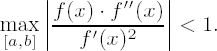
Then if xn € [a, b] is an approximation for a number r with f(r) = 0, then xn+1 := xn - f (xn)/f′ (xn) is a better approximation of r. The sequence defined in this way converges to the zero r of f (cf. [Endl], Section 7.3).
If we set f(x) := x2 - c with c > 0, then f(x) for x > 0 satisfies the above conditions for the convergence of the Newton method, and with
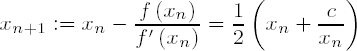
we obtain a sequence that converges to √c. Due to its favorable convergence behavior Newton's method is an efficient procedure for approximating square roots of rational numbers.
Since for our purposes we are interested in only the integer part r of √c, for which r2 ≤ c < (r + 1)2 holds, where c itself is assumed to be a natural number, we can limit ourselves to computing the integer parts of the elements of the sequence of approximations. We begin with a number x1 √c and continue until we obtain a value greater than or equal to its predecessor, at which point the predecessor is the desired value. It is naturally a good idea to begin with a number that is as close to √c as possible. For a CLINT object with value c and e :=
Algorithm for determining the integer part r of the square root of a natural number n > 0
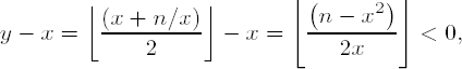
Set x ←

Set y ←
Output x and terminate the algorithm.
The proof of the correctness of this algorithm is not particularly difficult. The value of x decreases monotonically, and it is an integer and always positive, so that the algorithm certainly terminates. When this occurs, the condition y =
However,
in contradiction to the condition for terminating the process. Our assertion is therefore false, and we must have x = r. The following function, for determining the integer part of the square root, uses integer division with remainder for the operation y ←
Function | integer part of the square root of a |
Syntax: | |
Input: |
|
Output: |
|
void
iroot_l (CLINT n_l, CLINT floor_l)
{
  CLINT x_l, y_l, r_l;
  unsigned l;
Note
With the function ld_l() and a shift operation l is set to the value
l = (ld_l (n_l) + 1) >> 1;
  SETZERO_L (y_l);
  setbit_l (y_l, l);
  do
    {
cpy_l (x_l, y_l);div_l (n_l, x_l, y_l, r_l);
add_l (y_l, x_l, y_l);
shr_l (y_l);
}
while (LT_L (y_l, x_l));
cpy_l (floor_l, x_l);
}A generalization of the procedure makes possible the calculation of the integer part of the bth root of n, i.e.,
Algorithm for calculating the integer part of a bth root
Set
Set y ←
Output x as result and terminate the algorithm.
The implementation of the algorithm uses exponentiation modulo Nmax for the integer power in xb-1 in step 2:
Function | integer part of the bth root of a |
Syntax: |
|
Input: |
|
Output: |
|
int
introot_l (CLINT n_l, USHORT b, CLINT floor_l)
{
  CLINT x_l, y_l, z_l, junk_l, max_l;
  USHORT l;
  if (0 == b)
    {
      return −1;
    }
  if (EQZ_L (n_l))
    {
      SETZERO_L (floor_l);
      return E_CLINT_OK;
    }
  if (EQONE_L (n_l))
    {
      SETONE_L (floor_l);
      return E_CLINT_OK;
    }
  if (1 == b)
    {
      assign_l (floor_l, n_l);
      return E_CLINT_OK;
    }
  if (2 == b)
    {
      iroot_l (n_l, floor_l);
      return E_CLINT_OK;
    }
  /* step 1: set x_l ← 2⌈ld_l(n_l)/b⌉ */
  setmax_l (max_l);
  l = ld_l (n_l)/b;
  if (l*b != ld_l (n_l)) ++l;
  SETZERO_L (x_l);
  setbit_l (x_l, l);
/* step 2: loop to approximate the root until y_l ≥ x_l */
while (1)
{
umul_l (x_l, (USHORT)(b-1), y_l);
umexp_l (x_l, (USHORT)(b-1), z_l, max_l);
div_l (n_l, z_l, z_l, junk_l);
add_l (y_l, z_l, y_l);
udiv_l (y_l, b, y_l, junk_l);
if (LT_L (y_l, x_l))
{
assign_l (x_l, y_l);
}
else
{
break;
}
}
cpy_l (floor_l, x_l);
return E_CLINT_OK;
}To determine whether a number n is a bth root of another number, it suffices to raise the output value by introot_l() to the bth power and compare the result with n. If the values are unequal, then n is clearly not a root. For square roots one must, however, admit that this is not the most efficient method. There are criteria that in many cases can recognize such numbers that are not squares without the explicit calculation of root and square. Such an algorithm is given in [Cohe]. It uses four tables, q11, q63, q64, and q65, in which the quadratic residues modulo 11, 63, 64, and 65 are labeled with a "1" and the quadratic nonresidues with a "0":
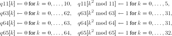
From the representation of the residue class ring as the absolute smallest residue system (cf. page 70) one sees that we obtain all squares in this way.
Algorithm for identifying an integer n > 0 as a square. In this case the square root of n is output (from [Cohe], Algorithm 1.7.3)
Set t ← n mod 64. If q64[t] = 0, then n is not a square and we are done. Otherwise, set r ← n mod (11 • 63 • 65).
If q63[r mod 63] = 0, then n is not a square, and we are done.
If q65[r mod 65] = 0, then n is not a square, and we are done.
If q11[r mod 11] = 0, then n is not a square, and we are done.
Compute q ←
This algorithm appears rather strange due to the particular constants that appear. But this can be explained: A square n has the property for any integer k that if it is a square in the integers, then it is a square modulo k. We have used the contrapositive: If n is not a square modulo k, then it is not a square in the integers. By applying steps 1 through 4 above we are checking whether n is a square modulo 64, 63, 65, or 11. There are 12 squares modulo 64, 16 squares modulo 63, 21 squares modulo 65, and 6 squares modulo 11, so that the probability that we are in the case that a number that is not a square has not been identified by these four steps is
It is only for these relatively rare cases that the test in step 5 is carried out. If this test is positive, then n is revealed to be a square, and the square root of n is determined. The order of the tests in steps 1 through 4 is determined by the individual probabilities. We have anticipated the following function in Section 6.5 to exclude squares as candidates for primitive roots modulo p.
Function | determining whether a |
Syntax: |
|
Input: |
|
Output: |
|
Return: | 1 if 0 otherwise |
static const UCHAR q11[11]=
  {1, 1, 0, 1, 1, 1, 0, 0, 0, 1, 0};
static const UCHAR q63[63]=
  {1, 1, 0, 0, 1, 0, 0, 1, 0, 1, 0, 0, 0, 0, 0, 0, 1, 0, 1, 0, 0, 0, 1,
    0, 0, 1, 0, 0, 1, 0, 0, 0, 0, 0, 0, 0, 1, 1, 0, 0, 0, 0, 0, 1, 0, 0,
    1, 0, 0, 1, 0, 0, 0, 0, 0, 0, 0, 0, 1, 0, 0, 0, 0};
static const UCHAR q64[64]=
{1, 1, 0, 0, 1, 0, 0, 0, 0, 1, 0, 0, 0, 0, 0, 0, 1, 1, 0, 0, 0, 0, 0,
0, 0, 1, 0, 0, 0, 0, 0, 0, 0, 1, 0, 0, 1, 0, 0, 0, 0, 1, 0, 0, 0, 0,
0, 0, 0, 1, 0, 0, 0, 0, 0, 0, 0, 1, 0, 0, 0, 0, 0, 0};
static const UCHAR q65[65]=
{1, 1, 0, 0, 1, 0, 0, 0, 0, 1, 1, 0, 0, 0, 1, 0, 1, 0, 0, 0, 0, 0, 0,
0, 0, 1, 1, 0, 0, 1, 1, 0, 0, 0, 0, 1, 1, 0, 0, 1, 1, 0, 0, 0, 0, 0,
0, 0, 0, 1, 0, 1, 0, 0, 0, 1, 1, 0, 0, 0, 0, 1, 0, 0, 1};
unsigned int
issqr_l (CLINT n_l, CLINT r_l)
{
CLINT q_l;
USHORT r;
if (EQZ_L (n_l))
{
SETZERO_L (r_l);
return 1;
}Note
The case q64[n_1 mod 64]
if (1 == q64[*LSDPTR_L (n_l) & 63])
    {
      r = umod_l (n_l, 45045); /* n_l mod (11•63•65) */
      if ((1 == q63[r % 63]) && (1 == q65[r % 65]) && (1 == q11[r % 11]))
Note
Note that evaluation of the previous expression takes place from left to right; cf.[Harb], Section 7.7
{
          iroot_l (n_l, r_l);
          sqr_l (r_l, q_l);
          if (equ_l (n_l, q_l))
            {
              return 1;
          }
       }
    }
  SETZERO_L (r_l);
  return 0;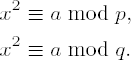
}Now that we have calculated square roots of whole numbers, or their integer parts, we turn our attention once again to residue classes, where we shall do the same thing, that is, calculate square roots. Under certain assumptions there exist square roots in residue class rings, though in general they are not uniquely determined (that is, an element may have more than one square root). Put algebraically, the question is to determine whether for an element
If gcd(a, m) = 1 and there exists a solution b with b2 ≡ a mod m, then a is called a quadratic residue modulo m. If there is no solution to the congruence, then a is called a quadratic nonresidue modulo m. If b is a solution to the congruence, then so is b + m, and therefore we can restrict our attention to those residues that differ modulo m.
Let us clarify the situation with the help of an example: 2 is a quadratic residue modulo 7, since 32 ≡ 9 ≡ 2 (mod 7), while 3 is a quadratic nonresidue modulo 5.
In the case that m is a prime number, then the determination of square roots modulo m is easy, and in the next chapter we shall present the functions required for this purpose. However, the calculation of square roots modulo a composite number depends on whether the prime factorization of m is known. If it is not, then the determination of square roots for large m is a mathematically difficult problem in the complexity class NP (see page 103), and it is this level of complexity that ensures the security of modern cryptographic systems.[21] We shall return to more elucidative examples in Section 10.4.4
The determination of whether a number has the property of being a quadratic residue and the calculation of square roots are two different computational problems each with its own particular algorithm, and in the following sections we will provide explanations and implementations. We first consider procedures for determining whether a number is a quadratic residue modulo a given number. Then we shall calculate square roots modulo prime numbers, and in a later section we shall give approaches to calculating square roots of composite numbers.
We plunge right into this section with a definition: Let p ≠ 2 be a prime number and a an integer. The Legendre symbol
(i) The number of solutions of the congruence x2 ≡ a (mod p) is 1 +

(ii) There are as many quadratic residues as nonresidues modulo p, namely (p - 1)/2.
(iii) a ≡ b (mod p)

(iv) The Legendre symbol is multiplicative:
(v)
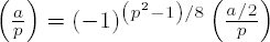
(vi)
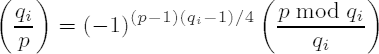
(vii) For an odd prime q, q ≠ p, we have
(viii)

The proofs of these properties of the Legendre symbol can be found in the standard literature on number theory, for example [Bund] or [Rose].
Two ideas for calculating the Legendre symbol come at once to mind: We can use the Euler criterion (vi) and compute a(p−1)/2 (mod p). This requires a modular exponentiation (an operation of complexity O (log3 p). Using the reciprocity law, however, we can employ the following recursive procedure, which is based on properties (iii), (iv), (vii), and (viii).
Recursive algorithm for calculating the Legendre symbol
If a = 1, then

If a is even, then
If a ≠ 1 and a = q1 ••• qk is the product of odd primes q1, . . . , qk, then
For each i we compute
by means of steps 1 through 3 (properties (iii), (iv), and (vii)).
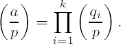
Before we examine the programming techniques required for computing the Legendre symbol we consider a generalization that can be carried out without the prime decomposition, such as would be required by the direct application of the reciprocity law in the version above (vii), which for large numbers takes an enormous amount of time (for the factoring problem see page 203). At that point we will be able to fall back on a nonrecursive procedure: For an integer a and an integer b = p1p2 ••• pk with not necessarily distinct prime factors piM the Jacobi symbol (or Jacobi-Kronecker, Kronecker-Jacobi, or Kronecker symbol)
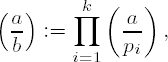
where
For the sake of completeness we set
If b is itself an odd prime (that is, k = 1), then the values of the Jacobi and Legendre symbols are the same. In this case the Jacobi (Legendre) symbol specifies whether a is a quadratic residue modulo b, that is, whether there is a number c with c2 ≡ a mod b, in which case
From the properties of the Legendre symbol we can conclude the following about the Jacobi symbol:
(i)
(ii) a ≡ c mod
(iii) For odd b > 0 we have

(iv) For odd a and b with b > 0 we have the reciprocity law (see (viii) above)
From these properties (see the above references for the proofs) of the Jacobi symbol we have the following algorithm of Kronecker, taken from [Cohe], Section 1.4, that calculates the Jacobi symbol (or, depending on the conditions, the Legendre symbol) of two integers in a nonrecursive way. The algorithm deals with a possible sign of b, and for this we set
Algorithm for calculating the Jacobi symbol of integers
If b = 0, output 1 if the absolute value |a| of a is equal to 1; otherwise, output 0 and terminate the algorithm.
If a and b are both even, output 0 and terminate the algorithm. Otherwise, set v ← 0, and as long as b is even, set v ← v + 1 and b ← b/2. If now v is even, set k ← 1; otherwise, set k ← (-1)(a2−1)/8. If b < 0, then set b ← -b. If a < 0, set k ← -k (cf. (iii)).
If a = 0, output 0 if b > 1, otherwise k, and terminate the algorithm. Otherwise, set v ← 0, and as long as a is even, set v ← v + 1 and a ← a/2. If now v is odd, set k ← (-1)(b2−1)/8 • k (cf. (iii)).
Set k ← (−1)(a−1)(b−1)/4•k, r ← |a|, a ← b mod r, b ← r, and go to step 3 (cf. (ii) and (iv)).
The run time of this procedure is O (log2N), where N ≥ a, b represents an upper bound for a and b. This is a significant improvement over what we achieved with the Euler criterion. The following tips for the implementation of the algorithm are given in Section 1.4 of [Cohe].
In both cases the explicit computation of a power can be avoided, which of course has a positive effect on the total run time.
We would like to clarify the first tip with the help of the following considerations: If k in step 2 is set to the value (-1)(a2−1)/8, then a is odd. The same holds for b in step 3. For odd a we have
or
so that 8 is a divisor of (a - 1)(a + 1) = a2 - 1. Thus (-1)(a2−1)/8 is an integer. Furthermore, we have (-1)(a2−1)/8 = (-1)((amod8)2−1)/8 (this can be seen by placing the representation a = k • 8 + r in the exponent). The exponent must therefore be determined only for the four values a mod 8 = ±1 and ±3, for which the results are 1, −1, −1, and 1. These are placed in a vector {0, 1, 0, −1, 0, −1, 0, 1}, so that by knowing a mod 8 one can access the value of (-1)((amod8)2−1)/8. Observing that a mod 8 can be represented by the expression a & 7, where again & is binary AND, then the calculation of the power is reduced to a few fast CPU operations. For an understanding of the second tip we note that (a & b & 2) ≠ 0 if and only if (a - 1)/2 and (b - 1)/2, and hence (a - 1)(b - 1)/4 , are odd.
Finally, we use the auxiliary function twofact_l(), which we briefly introduce here, for determining v and b in step 2, for the case that b is even, as well as in the analogous case for the values v and a in step 3. The function twofact_l() decomposes a CLINT value into a product consisting of a power of two and an odd factor.
Function: | decompose a |
Syntax: |
|
Input: |
|
Output: |
|
Return: | k (logarithm to base 2 of the two-part of |
int
twofact_l (CLINT a_l, CLINT b_l)
{
  int k = 0;
  if (EQZ_L (a_l))
    {
      SETZERO_L (b_l);
      return 0;
    }
  cpy_l (b_l, a_l);
  while (ISEVEN_L (b_l))
    {
      shr_l (b_l);
      ++k;
    }
  return k;
}
Thus equipped we can now create an efficient function jacobi_l() for calculating the Jacobi symbol.
Function: | calculate the Jacobi symbol of two |
Syntax: |
|
Input: |
|
Return: | ±1 (value of the Jacobi symbol of |
static int tab2[] = 0, 1, 0, −1, 0, −1, 0, 1;

int
jacobi_l (CLINT aa_l, CLINT bb_l)
{
  CLINT a_l, b_l, tmp_l;
  long int k, v;
Note
Step 1: The case bb_l = 0.
if (EQZ_L (bb_l))
  {
    if (equ_l (aa_l, one_l))
      {
return 1;
}
else
{
return 0;
}
}Note
Step 2: Remove the even part of bb_l.
if (ISEVEN_L (aa_l) && ISEVEN_L (bb_l))
  {
    return 0;
  }
cpy_l (a_l, aa_l);
cpy_l (b_l, bb_l);
v = twofact_l (b_l, b_l);
if ((v & 1) == 0)    /* v even? */
  {
   k = 1;
  }
else
  {
   k = tab2[*LSDPTR_L (a_l) & 7];    /* *LSDPTR_L (a_l) & 7 == a_l % 8 */
  }
Note
Step 3: If a_l = 0, then we are done. Otherwise, the even part of a_l is removed.
while (GTZ_L (a_l))
  {
    v = twofact_l (a_l, a_l);
    if ((v & 1) != 0)
      {
        k = tab2[*LSDPTR_L (b_l) & 7];
      }
Note
Step 4: Application of the quadratic reciprocity law.
if (*LSDPTR_L (a_l) & *LSDPTR_L (b_l) & 2)
      {
        k = -k;
      }
cpy_l (tmp_l, a_l);
mod_l (b_l, tmp_l, a_l);
cpy_l (b_l, tmp_l);
}
if (GT_L (b_l, one_l))
{
k = 0;
}
return (int) k;
}We now have an idea of the property possessed by an integer of being or not being a quadratic residue modulo another integer, and we also have at our disposal an efficient program to determine which case holds. But even if we know whether an integer a is a quadratic residue modulo an integer n, we still cannot compute the square root of a, especially not in the case where n is large. Since we are modest, we will first attempt this feat for those n that are prime. Our task, then, is to solve the quadratic congruence
where we assume that p is an odd prime and a is a quadratic residue modulo p, which guarantees that the congruence has a solution. We shall distinguish the two cases p ≡ 3 mod 4 and p ≡ 1 mod 4. In the former, simpler, case, x := a(p+1)/4 mod p solves the congruence, since
where for
The following considerations, taken from [Heid], lead to a general procedure for solving quadratic congruences, and in particular for solving congruences of the second case, p ≡ 1 mod 4: We write p - 1 = 2kq, with k ≥ 1 and q odd, and we look for an arbitrary quadratic nonresidue n mod p by choosing a random number n with 1 ≤ n < p and calculating the Legendre symbol
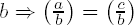
We set
Since by Fermat's little theorem we have a(p−1)/2 ≡ x2(p−1)/2 ≡ xp−1 ≡ 1 mod p for a and for a solution x of (10.11), and since additionally, for quadratic nonresidues n we have n(p−1)/2 ≡ −1 mod p (cf. (vi), page 221), we have
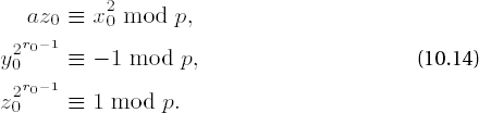
If z0 ≡ 1 mod p, then x0 is already a solution of the congruence (10.11). Otherwise, we recursively define numbers xi, yi, zi, ri such that
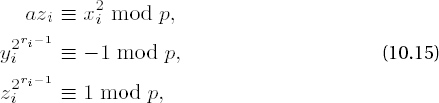
and ri > ri−1. After at most k steps we must have zi ≡ 1 mod p and that xi is a solution to (10.11). To this end we choose m0 as the smallest natural number such that z02m0 ≡ 1 mod p, whereby m0 ≤ r0 - 1. We set
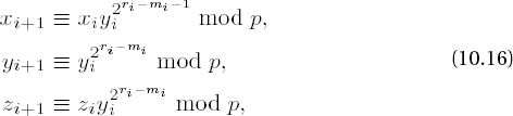
with
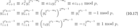
since
We have thus proved a solution procedure for quadratic congruence, on which the following algorithm of D. Shanks is based (presented here as in [Cohe], Algorithm 1.5.1).
Algorithm for calculating square roots of an integer a modulo an odd prime p
Write p - 1 = 2kq, q odd. Choose random numbers n until

Set x ← a(q−1)/2 mod p, y ← nq mod p, z ← a • x2 mod p, x ← a • x mod p, and r ← k.
If z ≡ 1 mod p, output x and terminate the algorithm. Otherwise, find the smallest m for which z2m ≡ 1 mod p. If m = r, then output the information that a is not a quadratic residue p and terminate the algorithm.
Set t ← y2r-m−1 mod p, y ← t2 mod p, r ← m mod p, x ← x • t mod p, z ← z • y mod p, and go to step 3.
It is clear that if x is a solution of the quadratic congruence, then so is -x mod p, since (-x)2 ≡ x2 mod p.
Out of practical considerations in the following implementation of the search for a quadratic nonresidue modulo p we shall begin with 2 and run through all the natural numbers testing the Legendre symbol in the hope of finding a nonresidue in polynomial time. In fact, this hope would be a certainty if we knew that the still unproved extended Riemann hypothesis were true (see, for example, [Bund], Section 7.3, Theorem 12, or [Kobl], Section 5.1, or [Kran], Section 2.10). To the extent that we doubt the truth of the extended Riemann hypothesis the algorithm of Shanks is probabilistic.
For the practical application in constructing the following function proot_l() we ignore these considerations and simply expect that the calculational time is polynomial. For further details see [Cohe], pages 33 f.
Function: | compute the square root of a modulo p |
Syntax: |
|
Input: |
|
Output: |
|
Return: | 0 if |
int
proot_l (CLINT a_l, CLINT p_l, CLINT x_l)
{
  CLINT b_l, q_l, t_l, y_l, z_l;
  int r, m;

  if (EQZ_L (p_l) || ISEVEN_L (p_l))
    {
      return −1;
    }
Note
If a_l == 0, the result is 0.
if (EQZ_L (a_l))
    {
      SETZERO_L (x_l);
      return 0;
    }
Note
Step 1: Find a quadratic nonresidue.
cpy_l (q_l, p_l);
  dec_l (q_l);
  r = twofact_l (q_l, q_l);
  cpy_l (z_l, two_l);
  while (jacobi_l (z_l, p_l) == 1)
    {
     inc_l (z_l);
    }
  mexp_l (z_l, q_l, z_l, p_l);
Note
Step 2: Initialization of the recursion.
cpy_l (y_l, z_l);
  dec_l (q_l);
  shr_l (q_l);
  mexp_l (a_l, q_l, x_l, p_l);
  msqr_l (x_l, b_l, p_l);
  mmul_l (b_l, a_l, b_l, p_l);
  mmul_l (x_l, a_l, x_l, p_l);
Note
Step 3: End of the procedure; otherwise, find the smallest m such that z2m ≡ 1 mod p.
mod _l (b_l, p_l, q_l);
  while (!equ_l (q_l, one_l))
    {
      m = 0;
      do
        {
          ++m;
          msqr_l (q_l, q_l, p_l);
        }
      while (!equ_l (q_l, one_l));

      if (m == r)
        {
          return −1;
        }
Note
Step 4: Recursion step for x, y, z, and r.
mexp2_l (y_l, (ULONG)(r - m - 1), t_l, p_l);
      msqr_l (t_l, y_l, p_l);
      mmul_l (x_l, t_l, x_l, p_l);
      mmul_l (b_l, y_l, b_l, p_l);
      cpy_l (q_l, b_l);
      r = m;
    }
  return 0;
}
The calculation of roots modulo prime powers pk can now be accomplished on the basis of our results modulo p. To this end we first consider the congruence
based on the following approach: Given a solution x1 of the above congruence x2 ≡ a mod p we set x := x1 + p • x2, from which follows

From this we deduce that for solving (10.18) we will be helped by a solution x2 of the linear congruence
Proceeding recursively one obtains in a number of steps a solution of the congruence x2 ≡ a mod pk for any k € •.
The ability to calculate square roots modulo a prime power is a step in the right direction for what we really want, namely, the solution of the more general problem x2 ≡ a mod n for a composite number n. However, we should say at once that the solution of such a quadratic congruence is in general a difficult problem. In principle, it is solvable, but it requires a great deal of computation, which grows exponentially with the size of n: The solution of the congruence is as difficult (in the sense of complexity theory) as factorization of the number n. Both problems lie in the complexity class NP (cf. page 103). The calculation of square roots modulo composite numbers is therefore related to a problem for whose solution there has still not been discovered a polynomial-time algorithm. Therefore, for large n we cannot expect to find a fast solution to this general case.
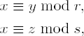
Nonetheless, it is possible to piece together solutions of quadratic congruences y2 ≡ a mod r and z2 ≡ a mod s with relatively prime numbers r and s to obtain a solution of the congruence x2 ≡ a mod rs. Here we will be assisted by the Chinese remainder theorem:
Given congruences x ≡ ai mod mi with natural numbers m1, . . . , mr that are pairwise relatively prime (that is, gcd (mi, mj) = 1 for i ≠ j) and integers a1, . . . , ar, there exists a common solution to the set of congruences, and furthermore, such a solution is unique modulo the product m1 • m2 ••• mr.
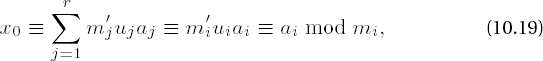
We would like to spend a bit of time in consideration of the proof of this theorem, for it contains hidden within itself in a remarkable way the promised solution: We set m := m1 •m2 ••• mr and mj′ := m/mj. Then mj′ is an integer and gcd mj′, mj = 1. From Section 10.2 we know that that there exist integers uj and vj with 1 = mj′uj + mj′vj, that is, mj′uj ≡ 1 mod mj, for j = 1, . . . , r and how to calculate them.
We then form the sum
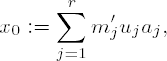
and since mj′uj ≡ 0 mod mi for i ≡ j, we obtain
and in this way have constructed a solution to the problem. For two solutions x0 ≡ ai mod mi and x1 ≡ ai mod mi we have x0 ≡ x1 mod mi. This is equivalent to the difference x0 - x1 being simultaneously divisible by all mi, that is, by the least common multiple of the mi. Due to the pairwise relative primality of the mi we have that the least common multiple is, in fact, the product of the mi, so that finally, we have that x0 ≡ x1 mod m holds.
We now apply the Chinese remainder theorem to obtain a solution of x2 ≡ a mod rs with gcd(r, s) = 1, where r and s are distinct odd primes and neither r nor s is a divisor of a, on the assumption that we have already obtained roots of y2 ≡ a mod r and z2 ≡ a mod s. We now construct as above a common solution to the congruences
by
x0 := (zur + yvs) mod rs,
where 1 ≡ ur + vs is the representation of the greatest common divisor of r and s. We thus have x02 ≡ a mod r and x02 ≡ a mod s, and since gcd(r, s) ≡ 1, we also have x02 ≡ a mod rs, and so we have found a solution of the above quadratic congruence. Since as shown above every quadratic congruence modulo r and modulo s possesses two solutions, namely ±y and ±z, the congruence modulo rs has four solutions, obtained by substituting in ±y and ±z above:
We have thus found in principle a way to reduce the solution of quadratic congruences x2 ≡ a mod n with n odd to the case x2 ≡ a mod p for primes p. For this we determine the prime factorization n = p1k1 ••• ptkt and then calculate the roots modulo the pi, which by the recursion in Section 10.4.2 can be used to obtain solutions of the congruences x2 ≡ a mod piki. As the crowning glory of all this we then assemble these solutions with the help of the Chinese remainder theorem into a solution of x2 ≡ a mod n. The function that we give takes this path to solving a congruence x2 ≡ a mod n. However, it assumes the restricted hypothesis that n = p • q is the product of two odd primes p and q, and first calculates solutions x1 and x2 of the congruences
From x1 and x2 we assemble according to the method just discussed the solutions to the congruence
and the output is the smallest square root of a modulo pq.
Function: | calculate the square root of a modulo p • q for odd primes p, q |
Syntax: | |
Input: |
|
Output: |
|
Return: | 0 if |
int
root_l (CLINT a_l, CLINT p_l, CLINT q_l, CLINT x_l)
 {
  CLINT x0_l, x1_l, x2_l, x3_l, xp_l, xq_l, n_l;
  CLINTD u_l, v_l;
  clint *xptr_l;
  int sign_u, sign_v;
Note
Calculate the roots modulo p_l and q_l with the function proot_l(). If a_l == 0, the result is 0.
if (0 != proot_l (a_l, p_l, xp_l) || 0 != proot_l (a_l, q_l, xq_l))
    {
      return −1;
    }
  if (EQZ_L (a_l))
    {
      SETZERO_L (x_l);
      return 0;
      }
Note
For the application of the Chinese remainder theorem we must take into account the signs of the factors u_l and v_l, represented by the auxiliary variables sign_u and sign_v, which assume the values calculated by the function xgcd_l(). The result of this step is the root x0.
mul_l (p_l, q_l, n_l);
  xgcd_l (p_l, q_l, x0_l, u_l, &sign_u, v_l, &sign_v);
  mul_l (u_l, p_l, u_l);
  mul_l (u_l, xq_l, u_l);
  mul_l (v_l, q_l, v_l);
  mul_l (v_l, xp_l, v_l);

  sign_u ≡ sadd (u_l, sign_u, v_l, sign_v, x0_l);

  smod (x0_l, sign_u, n_l, x0_l);
Note
Now we calculate the roots x1, x2, and x3.
sub_l (n_l, x0_l, x1_l);
  msub_l (u_l, v_l, x2_l, n_l);
  sub_l (n_l, x2_l, x3_l);
Note
The smallest root is returned as result.
xptr_l ≡ MIN_L (x0_l, x1_l);
  xptr_l ≡ MIN_L (xptr_l, x2_l);
  xptr_l ≡ MIN_L (xptr_l, x3_l);
  cpy_l (x_l, xptr_l);
  return 0;
}
From this we can now easily deduce an implementation of the Chinese remainder theorem by taking the code sequence from the above function and extending it by the number of congruences that are to be simultaneously solved. Such a procedure is described in the following algorithm, due to Garner (see [MOV], page 612), which has an advantage with respect to the application of the Chinese remainder theorem in the above form in that reduction must take place only modulo the mi, and not modulo m ≡ m1m2 ••• mr. This results in a significant savings in computing time.
Algorithm 1 for a simultaneous solution of a system of linear congruences x ≡ ai mod mi, 1 ≤i ≤ r, with gcd (mi, mj ) = 1 for i ≠ j
Set u ← a1, x ← u, and i ← 2.
Set Ci ← 1, j ← 1.
Set u ← mj−1 mod mi (computed by means of the extended Euclidean algorithm; see page 181) and Ci ← uCi mod mi.
Set j ← j + 1; if j ≤ i - 1, go to step 3.
Set u ← (ai - x) Ci mod mi, and
Set i ← i + 1; if i ≤ r, go to step 2. Otherwise, output x.
It is not obvious that the algorithm does what it is supposed to, but this can be shown by an inductive argument. To this end let r = 2. In step 5 we then have
It is seen at once that x ≡ a1 mod m1. However, we also have
To finish the induction by passing from r to r + 1 we assume that the algorithm returns the desired result xr for some r ≥ 2, and we append a further congruence x ≡ ar+1 mod mr+1. Then by step 5 we have
Here we have x ≡ xr ≡ ai mod mi for i = 1, . . . , r according to our assumption. But we also have
which completes the proof.
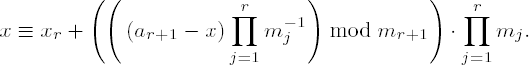
For the application of the Chinese remainder theorem in programs one function would be particularly useful, one that is not dependent on a predetermined number of congruences, but rather allows the number of congruences to be specified at run time. This method is supported by an adaptation of the above construction procedure, which does not, alas, have the advantage that reduction need take place only modulo mi, but it does make it possible to process the parameters ai and mi of a system of congruences with i = 1, . . . , r with variable r with a constant memory expenditure. Such a solution is contained in the following algorithm from [Cohe], Section 1.3.3.
Algorithm 2 for calculating a simultaneous solution of a system of linear congruences x ≡ ai mod mi, 1 ≤ i ≤ r, with gcd (mi, mj ) = 1 for i ≠ j
Set i ← 1, m ← m1, and x ← a1.
If i = r, output x and terminate the algorithm. Otherwise, increase i ← i+1 and calculate u and v with 1 = um + vmi using the extended Euclidean algorithm (cf. page 179).
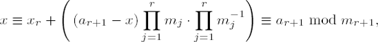
Set x ← umai + vmix, m ← mmi, x ← x mod m and go to step 2.
The algorithm immediately becomes understandable if we carry out the computational steps for three equations x = ai mod mi, i = 1, 2, 3: For i = 2 we have in step 2
and in step 3
In the next pass through the loop with i = 3 the parameters a3 and m3 are processed. In step 2 we then have
and in step 3

The summands u2m1m2a3 and v2m3u1m1a2 disappear in forming the residue x2 modulo m1; furthermore, v2m3 ≡ v1m2 ≡ 1 mod m1 by construction, and thus x2 ≡ a1 mod m1 solves the first congruence. Analogous considerations lead us to see that x2 also solves the remaining congruences.
We shall implement this inductive variant of the construction principle according to the Chinese remainder theorem in the following function chinrem_l(), whose interface enables the passing of coefficients of a variable number of congruences. For this a vector with an even number of pointers to CLINT objects is passed, which in the order a1, m1, a2, m2, a3, m3, . . . are processed as coefficients of congruences x ≡ ai mod mi. Since the number of digits of the solution of a congruence system x ≡ ai mod mi is of order
Function: | solution of linear congruences with the Chinese remainder theorem |
Syntax: | |
Input: |
|
Output: |
|
Return: |
1 if noofeq is 0 2 if mi are not pairwise relatively prime |
int
chinrem_l (unsigned int noofeq, clint** coeff_l, CLINT x_l)
{
  clint *ai_l, *mi_l;
  CLINT g_l, u_l, v_l, m_l;
  unsigned int i;
  int sign_u, sign_v, sign_x, err, error = E_CLINT_OK;
  if (0 == noofeq)
    {
      return 1;
    }
Note
Initialization: The coefficients of the first congruence are taken up.
cpy_l (x_l, *(coeff_l++));
cpy_l (m_l, *(coeff_l++));
Note
If there are additional congruences, that is, if no_of_eq > 1, the parameters of the remaining congruences are processed. If one of the mi_l is not relatively prime to the previous moduli occurring in the product m_l, then the function is terminated and 2 is returned as error code.
for (i = 1; i < noofeq; i++)
  {
   ai_l = *(coeff_l++);
   mi_l = *(coeff_l++);
   xgcd_l (m_l, mi_l, g_l, u_l, &sign_u, v_l, &sign_v);
   if (!EQONE_L (g_l))
     {
       return 2;
     }
Note
In the following an overflow error is recorded. At the end of the function the statusis indicated in the return of the error code stored in error.
err = mul_l (u_l, m_l, u_l);
if (E_CLINT_OK == error)
  {
    error = err;
  }
err = mul_l (u_l, ai_l, u_l);
if (E_CLINT_OK == error)
  {
    error = err;
  }
err = mul_l (v_l, mi_l, v_l);
if (E_CLINT_OK == error)
  {
    error = err;
  }
err = mul_l (v_l, x_l, v_l);
if (E_CLINT_OK == error)
  {
    error = err;
  }
Note
The auxiliary functions sadd() and smod() take care of the signs sign_u and sign_v (respectively sign_x) of the variables u_l and v_l (respectively 4).
sign_x = sadd (u_l, sign_u, v_l, sign_v, x_l);
      err = mul_l (m_l, mi_l, m_l);
      if (E_CLINT_OK == error)
        {
         error = err;
        }
      smod (x_l, sign_x, m_l, x_l);
    }
  return error;
}We come now to the promised examples for the cryptographic application of quadratic residues and their roots. To this end we consider first the encryption procedure of Rabin and then the identification schema of Fiat and Shamir.[22]
The encryption procedure published in 1979 by Michael Rabin (see [Rabi]) depends on the difficulty of calculating square roots in • pq. Its most important property is the provable equivalence of this calculation to the factorization problem (see also [Kran], Section 5.6). Since for encryption the procedure requires only a squaring modulo n, it is simple to implement, as the following demonstrates.
Ms. A generates two large primes p ≈ q and computes n = p • q.
Ms. A publishes n as a public key and uses the pair

With the public key nA a correspondent Mr. B can encode a message M € • n in the following way and send it to Ms. A.
Mr. B computes C := M2 mod nA with the function
msqr_l()on page 77 and sends the encrypted text C to A.To decode the message, A computes from C the four square roots Mi modulo nA, i = 1, . . . , 4, with the aid of the function
root_l()(cf. page 205), which here is modified so that not only the smallest but all four square roots are output.[23] One of these roots is the plain text M.
Ms. A now has the problem of deciding which of the four roots Mi represents the original plain text M. If prior to encoding the message B adds some redundant material, say a repetition of the last r bits, and informs A of this, then A will have no trouble in choosing the right text, since the probability that one of the other texts will have the same identifier is very slight.
Furthermore, redundancy prevents the following attack strategy against the Rabin procedure: If an attacker × chooses at random a number R € • ×nA and is able to obtain from A one of the roots Ri of X := R2 mod nA (no matter how he or she may motivate A to cooperate), then Ri
From nA = p • q | Ri2 - R2 = (Ri - R) (Ri + R) ≠ 0, however, one would have 1 ≠ gcd (R - Ri, nA) € {p, q}, and × would have broken the code with the factorization of nA (cf. [Bres], Section 5.2). On the other hand, if the plain text is provided with redundancy, then A can always recognize which root represents a valid plain text. Then A would at most reveal R (on the assumption that R had the right format), which for Mr. or Ms. ×, however, would be useless.
The avoidance of deliberate or accidental access to the roots of a pretended cipher text is a necessary condition for the use of the procedure in the real world.
The following example of the cryptographic application of quadratic residues deals with an identification schema published in 1986 by Amos Fiat and Adi Shamir. The procedure, conceived especially for use in connection with smart cards, uses the following aid: Let I be a sequence of characters with information for identifying an individual A, let m be the product of two large primes p and q, and let f (Z, n) → • m be a random function that maps arbitrary finite sequences of characters Z and natural numbers n in some unpredictable fashion to elements of the residue class ring • m. The prime factors p and q of the modulus m are known to a central authority, but are otherwise kept secret. For the identity represented by I and a yet to be determined k € • the central authority has now the task of producing key components as follows.
Compute numbers vi = f (I, i) € • m for some i ≥ k € •.
Choose k different quadratic residues vi1, . . . ,vikfrom among the vi and compute the smallest square roots Si1,...,v−1i1 of v−1i1, . . . , v−1i k in • m.
Store the values I and si1, . . . , sik securely against unauthorized access (such as in a smart card).
For generating keys sij we can use our functions jacobi_l() and root_l(); the function f can be constructed from one of the hash functions from Chapter 17, such as RIPEMD-160. As Adi Shamir once said at a conference, "Any crazy function will do."
With the help of the information stored by the central authority on the smart card Ms. A can now authenticate herself to a communication partner Mr. B.
A sends I and the numbers ij , j = 1, . . . , k, to
B.B generates vij = f (I, ij) € • m for j = 1, . . . , k. The following steps 3-6 are repeated for τ = 1, . . . , t (for a value t € • yet to be determined):
A chooses a random number rτ € • m and sends xτ = r2τ to
B.B sends a binary vector (eτ1, . . . , eτk) to
AA sends numbers • to B.
B verifies that
If A truly possesses the values si1, . . . ,sik, then in step 6

holds (all calculations are in • m), and A thereby has proved her identity to B. An attacker who wishes to assume the identity of A can with probability 2-kt guess the vectors (eτ1,...,eτk that B will send in step 4, and as a precaution in step 3 send the values
the size of the secret key;
the set of data to be exchanged between
AandB;the required computer time, measured as the number of multiplications.
Such parameters are given in [Fiat] for various values of k and t with kt = 72.
All in all, the security of the procedure depends on the secure storage of the values sij, on the choice of k and t, and on the factorization problem: Anyone who can factor the modulus m into the factors p and q can compute the secret key components sij, and the procedure has been broken. It is a matter, then, of choosing the modulus in such a way that it is not easily factorable. In this regard the reader is again referred to Chapter 17, where we discuss the generation of RSA moduli, subject to the same requirements.
A further security property of the procedure of Fiat and Shamir is that A can repeat the process of authentication as often as she wishes without thereby giving away any information about the secret key values. Algorithms with such properties are called zero knowledge processes (see, for example, [Schn], Section 32.11).
Not to stretch out the suspense, the largest known Mersenne prime, M11213, and, I believe, the largest prime known at present, has 3375 digits and is therefore just about T-281
Forty-First Known Mersenne Prime Found!!
http://www.mersenne.org/prime.htm (May 2004)The study of prime numbers and their properties is one of the oldest branches of number theory and one of fundamental significance for cryptography. From the seemingly harmless definition of a prime number as a natural number greater than 1 that has no divisors other than itself and 1 there arises a host of questions and problems with which mathematicians have been grappling for centuries and many of which remain unanswered and unsolved to this day. Examples of such questions are, "Are there infinitely many primes?" "How are the primes distributed among the natural numbers?" "How can one tell whether a number is prime?" "How can one identify a natural number that is not prime, that is, a number that is composite?" "How does one find all the prime factors of a composite number?"
That there are infinitely many primes was proven already by Euclid about 2300 years ago (see, for example, [Bund], page 5, and especially the amusing proof variant and the serious proof variant on pages 39 and 40). Another important fact, which up to now we have tacitly assumed, will be mentioned here explicitly: The fundamental theorem of arithmetic states that every natural number greater than 1 has a unique decomposition as a product of finitely many prime numbers, where the uniqueness is up to the order of the factors. Thus prime numbers are truly the building blocks of the natural numbers.
As long as we stick close to home in the natural numbers and do not stray among numbers that are too big for us to deal with easily we can approach a number of questions empirically and carry out concrete calculations. Take note, however, that the degree to which results are achievable depends in large measure on the efficiency of the algorithms used and the capacities of available computers.
A list of the largest numbers identified as prime, published on the Internet, demonstrates the impressive size of the most recent discoveries (see Table 10-1 and http://www.mersenne.org).
Table 10-1. The ten largest known primes (as of December 2004)
|
|
|
|
|---|---|---|---|
224 036 583 − 1 | 7 235 733 | Findley | 2004 |
220 996 011 − 1 | 6 320 430 | Shafer | 2003 |
213 466 917 - 1 | 4 053 946 | Cameron, Kurowski | 2001 |
26 972 593 - 1 | 2 098 960 | Hajratwala, Woltman, Kurowski | 1999 |
5 539 • 25 054 502 + 1 | 1 521 561 | Sundquist | 2003 |
23 021 377 − 1 | 909 526 | Clarkson, Woltman, Kurowski | 1998 |
22 976 221 − 1 | 895 932 | Spence, Woltman | 1997 |
1 372 930131 072 + 1 | 804 474 | Heuer | 2003 |
1 361 244131 072 + 1 | 803 988 | Heuer | 2004 |
1 176 694131 072 + 1 | 795 695 | Heuer | 2003 |
The largest known prime numbers are of the form 2p - 1. Primes that can be represented in this way are called Mersenne primes, named for Marin Mersenne (1588-1648), who discovered this particular structure of prime numbers in his search for perfect numbers. (A natural number is said to be perfect if it equals the sum of its proper divisors. Thus, for example, 496 is a perfect number, since 496 = 1 + 2 + 4 + 8 + 16 + 31 + 62 + 124 + 248.)
For every divisor t of p we have that 2t - 1 is a divisor of 2p - 1, since if p = ab, then
Therefore, we see that 2p - 1 can be prime only if p is prime. Mersenne himself announced in 1644, without being in possession of a complete proof, that for p ≤ 257 the only primes of the form 2p - 1 were those for the primes p € {2, 3, 5, 7, 13, 17, 19, 31, 67, 127, 257}. With the exception of p = 67 and p = 257, for which 2p - 1 is not prime, Mersenne's conjecture has been verified, and analogous results for many additional exponents have been established as well (see [Knut], Section 4.5.4, and [Bund], Section 3.2.12).
On the basis of the discoveries thus far of Mersenne primes one may conjecture that there exist Mersenne primes for infinitely many prime numbers p. However, there is as yet no proof of this conjecture (see [Rose], Section 1.2). An interesting overview of additional unsolved problems in the realm of prime numbers can be found in [Rose], Chapter 12.
Because of their importance in cryptographic public key algorithms prime numbers and their properties have come increasingly to public attention, and it is a pleasure to see how algorithmic number theory in regard to this and other topics has become popular as never before. The problems of identifying a number as prime and the decomposition of a number into its prime factors are the problems that have attracted the greatest interest. The cryptographic invulnerability of many public key algorithms (foremost among them the famous RSA procedure) is based on the fact that factorization is a difficult problem (in the sense of complexity theory), which at least at present is unsolvable in polynomial time.[25]
Until recently, the same held true, in a weakened form, for the identification of a number as prime if one were looking for a definitive proof that a number is prime. On the other hand, there are tests that determine, up to a small degree of uncertainty, whether a number is prime; furthermore, if the test determines that the number is composite, then that determination is definitive. Such probabilistic tests are, in compensation for the element of doubt, executable in polynomial time, and the probability of a "false positive" can be brought below any given positive bound, as we shall see, by repeating the test a sufficient number of times.
A venerable, but nonetheless still useful, method of determining all primes up to a given natural number N was developed by the Greek philosopher and astronomer Eratosthenes (276-195 B.C.E.; see also [Saga]), and in his honor it is known as the sieve of Eratosthenes. Beginning with a list of all natural numbers greater than 1 and less than or equal to N, we take the first prime number, namely 2, and strike from the list all multiples of 2 greater than 2 itself. The first remaining number above the prime number just used (2 in this case) is then identified as a prime p, whose multiples p (p + 2i), i = 0, 1, . . . , are likewise struck from the list. This process is continued until a prime number greater than √N is found, at which point the procedure is terminated. The numbers in the list that have not been struck are the primes less than or equal to N. They have been "caught" in the sieve.
We would like to elucidate briefly why it is that the sieve of Eratosthenes works as advertised: First, an induction argument makes it immediately plain that the next unstruck number above a prime is itself prime, since otherwise, the number would have a smaller prime divisor and thus would already have been struck from the list as a multiple of this prime factor. Since only composite numbers are struck, no prime numbers can be lost in the process.
Furthermore, it suffices to strike out only multiples of primes p for which p ≤ √N, since if T is the smallest proper divisor of N, then T ≤ √N. Thus if a composite number n √ N were to remain unstruck, then this number would have a smallest prime divisor p ≤ √n ≤ √N, and n would have been struck as a multiple of p, in contradiction to our assumption. Now we would like to consider how this sieve might be implemented, and as preparation we shall develop a programmable algorithm, for which we take the following viewpoint: Since except for 2 there are no even prime numbers, we shall consider only odd numbers as candidates for primality. Instead of making a list of odd numbers, we form the list fi, 1 ≤ i ≤
Sieve of Eratosthenes, algorithm for calculating all prime numbers less than or equal to a natural number N
Set L ←
If fi = 0, go to step 4. Otherwise, output p as a prime and set k ← s.
If k ≤ L, set fk ← 0, k ← k + p, and repeat step 3.
If i ≤ B, then set i ← i + 1, s ← s + 2p, p ← p + 2, and go to step 2. Otherwise, terminate the algorithm.
The algorithm leads us to the following program, which as result returns a pointer to a list of ULONG values that contains, in ascending order, all primes below the input value. The first number in the list is the number of prime numbers found.
Function: | prime number generator (sieve of Eratosthenes) |
Syntax: | |
Input: |
|
Return: | a pointer to vector of
|
ULONG *
genprimes (ULONG N)
{
  ULONG i, k, p, s, B, L, count;
  char *f;
  ULONG *primes;
Note
Step 1: Initialization of the variables. The auxiliary function ul_iroot() computes the integer part of the square root of a ULONG variable. For this it uses the procedure elucidated in Section 10.3. Then comes the allocation of the vector f for marking the composite numbers.
B = (1 + ul_iroot (N)) >> 1;
L = N >> 1;
if (((N & 1) == 0) && (N > 0))
  {
    --L;
  }
if ((f = (char *) malloc ((size_t) L+1)) == NULL)
  {
    return (ULONG *) NULL;
  }
for (i = 1; i <= L; i++)
  {
    f[i] = 1;
  }
p = 3;
s = 4;
Note
Steps 2, 3, and 4 constitute the actual sieve. The variable i represents the numerical value 2i + 1.
for (i = 1; i <= B; i++)
  {
    if (f[i])
      {
        for (k = s; k <= L; k += p)
          {
            f[k] = 0;
          }
        }
    s += p + p + 2;
    p += 2;
}
Note
Now the number of primes found is reported, and a field of ULONG variables of commensurate size is allocated.
for (count = i = 1; i <= L; i++)
  {
    count += f[i];
  }
if ((primes = (ULONG*)malloc ((size_t)(count+1) * sizeof (ULONG))) == NULL)
  {
     return (ULONG*)NULL;
  }
Note
The field f[] is evaluated, and all the numbers 2i + 1 marked as primes are stored in the field primes. If N ≥ 2, then the number 2 is counted as well.
for (count = i = 1; i <= L; i++)
  {
    if (f[i])
      {
        primes[++count] = (i << 1) + 1;
      }
  }
if (N < 2)
  {
    primes[0] = 0;
  }
else
  {
    primes[0] = count;
    primes[1] = 2;
  }
  free (f);
  return primes;
}
To determine whether a number n is composite it is sufficient, according to what we have said above, to institute a division test that divides n by all prime numbers less than or equal to √n. If one fails to find a divisor, then n is itself prime; the prime test divisors are given to us by the sieve of Eratosthenes. However, this method is not practicable, since the number of primes that have to be tested becomes rapidly too large. In particular, we have the prime number theorem , formulated as a conjecture by A. M. Legendre, that the number π (x) of primes p, 2 ≤ p ≤ x, approaches x/ ln x asymptotically as x goes to infinity (see, for example, [Rose], Chapter 12).[26] A few values of the number of primes less than a given x will help to make clear the size of numbers we are dealing with. Table 10-2 gives the values of both π (x), the actual number of primes less than or equal to x, and the asymptotic approximation x/ ln x. The question mark in the last cell indicates a number to be filled in by the reader.;-)
Table 10-2. The number of primes up to various limits x
x | 102 | 104 | 108 | 1016 | 1018 | 10100 |
|---|---|---|---|---|---|---|
x/ ln x | 22 | 1,086 | 5,428,681 | 271,434,051,189,532 | 24,127,471,216,847,323 | 4 × 1097 |
π (x) | 25 | 1,229 | 5,761,455 | 279,238,341,033,925 | 24,739,954,287,740,860 | ? |
The number of necessary calculations for the division test of x grows almost with the number of digits of x in the exponent. Therefore, the division test alone is not a practicable method for determining the primality of large numbers. We shall see, in fact, that the division test is an important aid in connection with other tests, but in principle we would be content to have a test that gave information about the primality of a number without revealing anything about its factorization. An improvement in the situation is offered by the little theorem of Fermat, which tells us that for a prime p and all numbers a that are not multiples of p the congruence ap−1 ≡ 1 mod p holds (see page 177).
From this fact we can derive a primality test, called the Fermat test: If for some number a we have gcd(a, n) ≠ 1 or gcd(a, n) = 1 and 1
We must face the fact that the converse of Fermat's little theorem does not hold: Not every number n with gcd(a, n) = 1 and an−1 ≡ 1 mod n for 1 ≤ a ≤ n - 1 is prime. There exist composite numbers n that pass the Fermat test as long as a and n are relatively prime. Such numbers are called Carmichael numbers, named for their discoverer, Robert Daniel Carmichael (1879-1967). The smallest of these curious objects are
All Carmichael numbers have in common the property that each of them possesses at least three different prime factors (see [Kobl], Chapter 5). It was only in the early 1990s that it was proven that there are infinitely many Carmichael numbers (see [Bund], Section 2.3).
The relative frequency of numbers less than n that are relatively prime to n is
(for the Euler (phis) function see page 177), so that the proportion of numbers that are not relatively prime to n is close to 0 for large n. Therefore, in most cases one must run through the Fermat test very often to determine that a Carmichael number is composite. Letting a run through the range 2 ≤ a ≤ n - 1, eventually, one encounters the smallest prime divisor of n, and it is only when a assumes this value that n is exposed as composite.
In addition to the Carmichael numbers there are further odd composite numbers n for which there exist natural numbers a with gcd(a, n) = 1 and an−1 ≡ 1 mod n. Such numbers are known as pseudoprimes to the base a. To be sure, one can make the observation that there are only a few pseudoprimes to the bases 2 and 3, or that, for example, up to 25 × 109 there are only 1770 integers that are simultaneously pseudoprimes to the bases 2, 3, 5, and 7 (see [Rose], Section 3.4), yet the sad fact remains that there is no general estimate of the number of solutions of the Fermat congruence for composite numbers. Thus the problem with the Fermat test is that the uncertainty as to whether the method of random tests will reveal a composite number as such cannot be correlated with the number of tests.
However, such a connection is offered on the basis of the Euler criterion (see Section 10.4.1): For an odd prime p and for all integers a that are not multiples of p, we have
where
| If for a natural number n there exists an integer a with gcd(a, n) = 1 and |
The required computational expenditure for establishing this criterion is the same as that for the Fermat test, namely O log3 n.
As with the Fermat test, where there is the problem of pseudoprimes, there exist integers n that for certain a satisfy the Euler criterion although they are composite. Such n are called Euler pseudoprimes to the base a. An example is n = 91 = 7•13 to the bases 9 and 10, for which we have
An Euler pseudoprime to a base a is always a pseudoprime to the base a (see page 221), since by squaring
There is, however, no counterpart to the Carmichael numbers for the Euler criterion, and based on the following observations of R. Solovay and V. Strassen we can see that the risk of a false test result for Euler pseudoprimes is favorably bounded from above.
(i) For a composite number n the number of integers a relatively prime to n for which
(ii) The probability that for a composite number n and k randomly selected numbers a1,...,ak relatively prime to n one has
These results make it possible to implement the Euler criterion as a probabilistic primality test, where "probabilistic" means that if the test returns that result "n is not prime," then this result is definitive, but it is only with a certain probability of error that we may infer that n is in fact prime.
Algorithm: Probabilistic primality test à la Solvay-Strassen for testing a natural number n for compositeness
Choose a random number a ≤ n - 1 with gcd(a, n) = 1.
If has
This test requires computation time O (log3 n) for the calculation of the exponent and the Jacobi symbol. By repeated application of this test we can reduce the probability of error in step (ii). For example, for k = 60 we obtain a vanishingly small probability of error less than 2−60 ≈ 10−18, and D. Knuth has indicated that this value is less than that of a transient hardware error, caused, for example, by an alpha particle that has found its way into the CPU or memory of a computer and thereby switched the value of a bit.
We might be satisfied with this test, since we have control over the probability of error and we have efficient algorithms for all the required computations. However, there are results that lead to a more efficient algorithm. For this we would like to introduce a few considerations that will improve our understanding of the most widely used probabilistic primality tests
Let us make the hypothesis that n is prime. Then by Fermat's little theorem we have an−1 ≡ 1 mod n for integers a that are not multiples of n. The square root of an−1 mod n can assume only the value 1 or −1, since these are the only solutions of the congruence x2 ≡ 1 mod n (see Section 10.4.1). If we also compute from an−1 mod n the successive square roots
one after another until (n - 1)/2t is odd, and if in the process we arrive at a residue not equal to 1, then this residue must have the value −1, for otherwise, n cannot be prime, which we have hypothesized. For the case that the first square root different from 1 has the value −1, we stick by our hypothesis that n is prime. If n is nevertheless composite, then we shall call n on the basis of this special property a strong pseudoprime to the base a. Strong pseudoprimes to a base a are always Euler pseudoprimes to the base a (see [Kobl], Chapter 5).
We assemble all of this into the following probabilistic primality test, though for the sake of efficiency we shall first compute the power b = a(n-1)/2t mod n with odd (n - 1)/2t, and if this is not equal to 1, we continue to square b until we obtain a value of ±1 or have reached a(n-1)/2 mod n. In the last case we must have either b = −1 or that n is composite. The idea of shortening the algorithm so that the last square does not have to be calculated has been taken from [Cohe], Section 8.2.
Probabilistic primality test à la Miller-Rabin for odd integers n > 1
Determine q and t with n - 1 = 2tq, with q odd.
Choose a random integer a, 1 < a < n. Set e ← 0, b ← aq mod n. If b = 1, output "n is probably prime" and terminate the algorithm.
As long as we have b

With a running time of O(log3n) for the exponentiations, the Miller-Rabin test (MR test for short) has complexity the same order of magnitude as the Solovay-Strassen test.
The existence of strong pseudoprimes means that the Miller-Rabin primality test offers us certainty only about the compositeness of numbers. The number 91, which we trotted out above as an example of an Euler pseudoprime (to base 9) is also—again to base 9—a strong pseudoprime. Further examples of strong pseudoprimes are
These two numbers are the only pseudoprimes below 1013 to the prime bases 2, 3, 5, 7, and 11 (see [Rose], Section 3.4).
Fortunately, the number of bases of strong pseudoprimes is again diminished by these numbers themselves. M. Rabin has proved that for a composite number n there are fewer than n/4 bases a, 2 ≤ a ≤ n - 1, to which n is a strong pseudoprime (see [Knut], Section 4.5.4, Exercise 22, and [Kobl], Chapter 5). From this we obtain with k-fold repetition of the test with k randomly chosen bases a1, . . . , ak a probability smaller than 4-k that a strong pseudoprime has been falsely accepted as a prime. Therefore, for the same amount of work, the Miller-Rabin test is superior to the Solovay-Strassen test, which with k repetitions has probability of error bounded by 2-k.
In practice, the Miller-Rabin test does much better than advertised, since the actual probability of error is in most cases much smaller than that guaranteed by the theorem of Rabin (see [MOV], Section 4.4, and [Schn], Section 11.5).
Before we get down to implementing the Miller-Rabin test, we look at two approaches to improving efficiency.
By beginning the Miller-Rabin test with a division sieve that divides the prime candidates by small primes, we obtain an advantage: If a factor is found in the process, then the candidate can be eliminated from consideration without the expense of a Miller-Rabin test. The question at once presents itself as to how many prime numbers would be optimal to divide by before undertaking the MR test. We give a recommendation due to A. K. Lenstra: The greatest efficiency is achieved if one divides by the 303 prime numbers less than 2000 (see [Schn], Section 11.5). The reason for this arises from the observation that the relative frequency of odd numbers without prime divisors less than the bound n is about 1.12/ln n. Dividing by prime numbers under 2000 eliminates about 85 percent of all composite numbers without using the MR test, which is then used only on the remaining candidates.
Each division by a small divisor requires computation time of order only O(ln n). We make use of an efficient division routine especially for small divisors and use it in instituting the division sieve.
The division sieve is implemented in the following function sieve_l(). It, in turn, uses the primes less than 65536 stored in the field smallprimes[NOOFSMALLPRIMES]. The primes are stored as differences, where for each prime only a byte of storage is required. The diminished access to these primes is not a serious problem, since we are using them in their natural order. The case that the candidate itself is a small prime and is contained in the prime number table must be specially indicated.
Finally, we profit from the exponentiation function for small bases (see Chapter 6) by applying the MR test with small primes 2, 3, 5, 7, 11, . . . < B instead of randomly selected bases. According to experience this in no way impairs the results of the test.
We now introduce the division sieve. The function uses the division routine for short divisors that we developed for the function div_l().
Function: | division sieve |
Syntax: |
|
Input: |
|
Return: | prime factor, if one is found 1, if the candidate itself is prime 0, if no factor is found |
USHORT
sieve_l (CLINT a_l, unsigned int no_of_smallprimes)
{
  clint *aptr_l;
  USHORT bv, rv, qv;
  ULONG rhat;
  unsigned int i = 1;
Note
For the sake of completeness we first test whether a_1 is a multiple of 2. If, in fact, a_1 has the value 2, then 1 is returned, while if a_1 is greater than 2 and is even, then 2 is returned as a factor.
if (ISEVEN_L (a_l))
  {
    if (equ_l (a_l, two_l))
      {
        return 1;
      }
    else
      {
        return 2;
      }
  }
bv = 2;
do
  {
Note
The prime numbers are computed by successive addition of the numbers stored in smallprimes[] and stored in bv. The first prime that serves as a divisor is 3. We use the code of the fast routine for division by a USHORT (see Section 4.3).
rv = 0;
bv += smallprimes[i];
for (aptr_l = MSDPTR_L (a_l); aptr_l >= LSDPTR_L (a_l); aptr_l--)
  {
    qv = (USHORT)((rhat = ((((ULONG)rv) << BITPERDGT) + (ULONG)*aptr_l)) / bv);
    rv = (USHORT)(rhat - (ULONG)bv * (ULONG)qv);
  }
}
while (rv != 0 && ++i <= no_of_smallprimes);
Note
If an actual divisor was found (rv == 0 and bv ≠ a_l; otherwise, a_l itself is prime!), this is returned. If a_l is itself a small prime, then 1 is returned. Otherwise, 0 is returned.
if (0 == rv)
  }
    if (DIGITS_L (a_l) == 1 && *LSDPTR_L (a_l) == bv)
      }
        bv = 1;
      }
    /* else: result in bv is a prime factor of a_l */
  }
else /* no factor of a_l was found */
  }
    bv = 0;
  }
return bv;
}
The function sieve_l() can be used for splitting off prime factors under 65536 from CLINT objects. To enable this, the macro SFACTOR_L(n_l) is defined in flint.h, which uses the call sieve_l(n_l, NOOFSMALLPRIMES) to test divide n_l by the primes stored in smallprimes[]; SFACTOR_L() returns the same value as sieve_l(). By repeated calls to SFACTOR_L() with subsequent division by the factors found, integers below 232, that is, integers that can be represented by the standard integer types, can be completely factored. If no factor is found, then we are dealing with a prime number.
The full-blown test function prime_l() integrates the division sieve and the Miller-Rabin test. To retain maximum flexibility the function is constituted in such a way that the number of divisions in the pretest and the number of passes through the Miller-Rabin test can be passed as parameters. To simplify the situation in applications, the macro ISPRIME_L(CLINT n_l) can be used, which in turn calls the function prime_l() with preset parameters.
There is differing advice in the literature in relation to the open question of how many repetitions of the Miller-Rabin test should be made in order to ensure reliable results. For example, [Gord] and [Schn] recommend five repetitions for cryptographic purposes, while the algorithm in [Cohe] prescribes 25 passes. In [Knut], the recommendation is that in 25 passes through the test, the number of errors for a set of a billion candidates accepted as prime numbers is under 10−6, although the value 25 is not explicitly endorsed, and he asks the philosophical question, "Do we really need to have a rigorous proof of primality?"[28]
For the application area of digital signatures, there is the opinion that error probabilities less than 2−80 ≈ 10−24 in the generation of prime numbers is acceptable (in Europe, the bound 2−60 ≈ 10−18 is also under discussion), so that errors are almost entirely excluded even when large numbers of keys are generated. In [RegT] it is suggested that in 2010,the threshold value should be lowered to 2−100. Applied to the estimate of the probability of error by Rabin, this would mean that 40, respectively 30, rounds of Miller-Rabin tests would be run, with longer calculation times as the size of the numbers being tested grows. In fact, however, there exist very much sharper estimates that depend not only on the number of passes, but also on the length of the prime number candidate (see [DaLP] and [Burt]). In [DaLP], the following inequalities are proved, where pl,k denotes the probability that a randomly selected odd number with l binary digits that is declared prime after k passes through the Miller-Rabin test is actually composite:
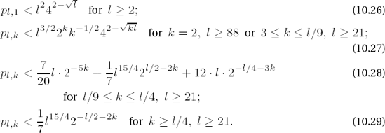
From these inequalities we can calculate what probabilities we can get below with how many passes of the Miller-Rabin test for a given number of digits, or how many passes are necessary to get below given probabilities of error. The results are far below those of Rabin, according to whom k repetitions are necessary to reach a probability of error beneath 4-k. Table 10-3 shows values of k necessary to reach probabilities below 2−80 and 2−100 as a function of the number l of binary digits of the numbers being tested.
Table 10-3. The number k of passes through the Miller-Rabin test to achieve probabilities of error less than 2−80 and 2−100 as a function of the number l of binary digits (after [DaLP]).
|
| ||
|---|---|---|---|
l | k | l | k |
49 | 37 | 49 | 47 |
73 | 32 | 73 | 42 |
105 | 25 | 105 | 35 |
137 | 19 | 132 | 29 |
197 | 15 | 198 | 23 |
220 to 234 | 13 | 223 | 20 |
235 to 251 | 12 | 242 | 18 |
252 to 272 | 11 | 253 | 17 |
273 to 299 | 10 | 265 | 16 |
300 to 331 | 9 | 335 | 12 |
332 to 374 | 8 | 480 to 542 | 8 |
375 to 432 | 7 | 543 to 626 | 7 |
433 to 513 | 6 | 627 to 746 | 6 |
514 to 637 | 5 | 747 to 926 | 5 |
638 to 846 | 4 | 927 to 1232 | 4 |
847 to 1274 | 3 | 1233 to 1853 | 3 |
1275 to 2860 | 2 | 1854 to 4095 | 2 |
≥ 2861 | 1 | ≥ 4096 | 1 |
The effect of using the division sieve before the Miller-Rabin test is not considered in inequalities (10.26) through (10.29). Since the sieve greatly reduces the relative frequency of composite candidates, one may expect that the probabilities of error for a given choice of l and k would be further reduced.
For a discussion of the subtle problems of conditional probabilities in relation to the probability of error in the generation of randomly selected prime numbers, see [BCGP] and [MOV], Section 4.4.
In the following function prime_l, the values from Table 10-3 will be considered. We use the exponentiation function wmexpm_l(), which combines Montgomery reduction with the advantages that accrue from exponentiation of small bases (see Chapter 6).
Function: | probabilistic primality test à la Miller-Rabin with division sieve |
Syntax: |
|
Input: |
|
Return: | 1 if the candidate is "probably" prime 0 if the candidate is composite or equal to 1 |
int
prime_l (CLINT n_l, unsigned int no_of_smallprimes, unsigned int iterations)
{
  CLINT d_l, x_l, q_l;
  USHORT i, j, k, p;
  int isprime = 1;

  if (EQONE_L (n_l))
    {
      return 0;
    }
Note
Now the division test is executed. If a factor is found, then the function is terminated with 0 returned. If 1 is returned by sieve_l(), indicating that n_l is itself prime, then the function is terminated with return value 1. Otherwise, the Miller-Rabin test is carried out.
k = sieve_l (n_l, no_of_smallprimes);
if (1 == k)
  {
    return 1;
  }
if (1 < k)
  {
    return 0;
  }
else
  {
    if (0 == iterations)
Note
If iterations == 0 is passed as parameter, then based on the number of digits of n_l, the optimized number of iterations for coming in under the bound of 2−80 is determined.
{
  k = ld_l (n_l);
  if (k < 73) iterations = 37;
  else if (k < 105) iterations = 32;
  else if (k < 137) iterations = 25;
  else if (k < 197) iterations = 19;
  else if (k < 220) iterations = 15;
  else if (k < 235) iterations = 13;
  else if (k < 253) iterations = 12;
  else if (k < 275) iterations = 11;
  else if (k < 300) iterations = 10;
  else if (k < 332) iterations = 9;
  else if (k < 375) iterations = 8;
  else if (k < 433) iterations = 7;
  else if (k < 514) iterations = 6;
  else if (k < 638) iterations = 5;
  else if (k < 847) iterations = 4;
  else if (k < 1275) iterations = 3;
  else if (k < 2861) iterations = 2;
  else iterations = 1;
}
Note
Step 1. The decomposition of n - 1 as n - 1 = 2kq with odd q is carried out by the function twofact_l(). The value n - 1 is retained in d_l.
cpy_l (d_l, n_l);
dec_l (d_l);
k = (USHORT)twofact_l (d_l, q_l);
p = 0;
i = 0;
isprime = 1;
do
  {
Note
Step 2. The bases p are formed from the differences stored in the field smallprimes[]. For the exponentiation we use the Montgomery function wmexpm_l, since the base is always of type USHORT and, after the pretest with the division sieve of the prime candidate n_l, always odd. If afterwards the power in x_l is equal to 1, then the next test iteration begins.
p += smallprimes[i++];
wmexpm_l (p, q_l, x_l, n_l);
if (!EQONE_L (x_l))
  {
    j = 0;
Note
Step 3. Squaring, as long as x_l is different from ±1 and k - 1 iterations have not yet been executed.
while (!EQONE_L (x_l) && !equ_l (x_l, d_l) && ++j < k)
  {
      msqr_l (x_l, x_l, n_l);
     }
if (!equ_l (x_l, d_l))
  {
    isprime = 0;
  }
 }
}while ((--iterations > 0) && isprime); return isprime; } }
For the cases in which definitive test results are required, the APRCL test, published in 1981 by its developers L. Adleman, C. Pomerance, R. Rumely, H. Cohen, and A. K. Lenstra, shows the direction of development of such tests. H. Riesel praised this test as a breakthrough, proving that fast, generally applicable, definitive primality tests were possible (see [Ries], page 131). The test determines the primality property of an integer n in time of order O ((ln n)C ln ln ln n) for a suitable constant C. Since the exponent ln ln ln n behaves like a constant for all practical purposes, it can be considered a polynomial-time procedure, and integers with several hundreds of decimal digits can have their primality or lack thereof determined definitively in times that are otherwise achieved only by probabilistic tests.[29] The algorithm, which uses analogues of Fermat's little theorem for higher algebraic structures, is theoretically complicated and difficult to implement. For further information see [Cohe], Chapter 9, or the original article cited therein, as well as the extensive explication in [Ries].
One might also ask whether one would obtain a definitive proof of primality by testing sufficiently many bases with the Miller-Rabin test. In fact, G. Miller has proved, on the assumption of the extended Riemann hypothesis (see page 200) that an odd natural number n is prime if and only if for all bases a, 1 ≤ a ≤ C • ln2 n, the Miller-Rabin test indicates the primality of n (the constant C is specified in [Kobl], Section 5.2, as 2). Used in this way the Miller-Rabin test is a deterministic polynomial-time primality test that uses about 106 iterations, for primes of about 1024 binary digits, to produce a definitive answer. If we suppose 10−3 seconds for each iteration (this is the order of magnitude for the time required for an exponentiation on a fast PC; cf. Appendix D), then a definitive test would take about an hour. Considering that there is an unproven hypothesis to be reckoned with, this theoretical result will satisfy neither the mathematical purists nor the computational pragmatists interested in fast procedures.
A surprising mathematical breakthrough occurred in 2002, when Maninda Agrawal, Neeraj Kayal, and Nitin Saxena, of the Indian Institute of Technology, in Kanpur, published an algorithm that provided a definitive proof of primality in polynomial time, thereby proving that the problem of recognizing a number to be prime belongs in the computational complexity class P. The algorithm was declared "brilliant and beautiful" by Carl Pomerance. The proof is elegant and surprisingly without any deep complexity, in contrast to what had been supposed, since a solution to the problem had been sought for centuries. Above all, we note that the proof does not rely on any unproven conjectures (see [AgKS]).
AKS algorithm for determining whether an integer n is prime
If n is a power of a natural number, go to step 8.
Set r ← 2.
If gcd(r, n) ≠ = 1, go to step 8.
If r is not prime, go to step 5. Otherwise, let q be the largest prime factor of r - 1. If
![The number k of passes through the Miller-Rabin test to achieve probabilities of error less than 2−80 and 2−100 as a function of the number l of binary digits (after [DaLP]).](http://imgdetail.ebookreading.net/software_development/3/9781590595022/9781590595022__cryptography-in-c__9781590595022__figs__U10123.png)
Set r ← r + 1 and go to step 3.
If for some a in the set
![The number k of passes through the Miller-Rabin test to achieve probabilities of error less than 2−80 and 2−100 as a function of the number l of binary digits (after [DaLP]).](http://imgdetail.ebookreading.net/software_development/3/9781590595022/9781590595022__cryptography-in-c__9781590595022__figs__U10125.png)
Output "n is prime."
Output "n is composite."
To exclude powers of natural numbers in step 1 of the AKS test it suffices to test whether
The AKS algorithm is based on a variant of Fermat's little theorem together with the binomial theorem, according to which for 1 < n € • and a € • ×n, the integer n is prime precisely when in the polynomial ring •n[X ] (see [AgKS], page 2), one has
A test based on this fact for an element a of • n[X] would then be able to determine definitively whether an integer n is prime. However, there would be considerable computation to determine the n coefficients of the polynomial (X + a)n, even more than in applying the sieve of Eratosthenes. Following the idea of Agrawal, Kayal, and Saxena, it turns out that both sides of equation (10.30) can be reduced modulo (Xr - 1) for a suitable value of r. If for sufficiently many values of a one has the equality
in the ring •n[x]/ (Xr - 1), then n is prime. Conversely, for a composite number n, there exist values of a and r such that (X + a)n ≠ (Xn + a) in •n[x]/ (Xr - 1). What is decisive here is that such values of a and r can be found in polynomial time if n is not prime, while if n is prime, it can be determined in polynomial time that such values do not exist. The size of the polynomial coefficients are bounded by r, and thus the calculation is faster, the smaller r is. If r is of order log n, the polynomial residue can be computed in polynomial time.
Agrawal, Kayal, and Saxena showed that suitable values of r can be found of size O (log5 n) and that the AKS test must be run only for values 1 ≥ a ≥ 2√r log n. The running time of the AKS test is therefore polynomial in log2 n, given by O (log7.5+ε n).[31] The problem is solved.
There remains the fascinating question what practical relevance the AKS test has from the point of view of cryptography: The expected calculation time determines whether it is of any practical use.
Crandall gives the values in Table 10-4 for small values of n from a small experimental C implementation on a "decent workstation."
Table 10-4. Approximate calculation times for the AKS test, after [CrPa]
n |
|
|---|---|
70 001 | 3 seconds |
700 001 | 15 seconds |
2 147 483 647 | 200 seconds |
1125 899 906 842 679 | 4000 seconds (ca. 1 hour) |
618 970 019 642 690 137 449 562 111 | 100 000 seconds (ca. 1 day) |
The times in the table correspond to about 10−6 log6 n seconds. An implementation by F. Bornemann based on the Pari-GP library requires nine seconds on a 1.7-GHz PC for proving the primality of 628 363 443 011 (see http://www-m3.ma.tum.de/m3/ftp/Bornemann/PARI/aks2.txt). The running time for a 512-bit prime number would then take several days. We thus obtain a definitive result, whose certainty we can approach only asymptotically using probabilistic primality tests. Since we can make the remaining probability of error, say by using the Miller-Rabin test, arbitrarily small, the disadvantage of not having that last bit of certainty is not very large in practice.
In sum, we should recognize that the AKS test represents a sensational result from the point of view of complexity theory, but that the Miller-Rabin test will continue to be the test of choice for cryptographic applications due to its enormous advantage in speed, even if Henri Cohen seems to be answering the above-quoted question of Knuth when he categorically asserts ([Cohe], Section 8.2), "Primality testing, however, requires rigorous mathematical proofs."
[19] In this case • p is in fact a field, since both (• p, +) and (•
[20] The little Fermat theorem states that for a prime number p and for any integer a one has ax ≡ a mod p. If p is not a divisor of a, then ap−1 ≡ 1 mod p (see [Bund], Chapter 2, §3.3). The little theorem of Fermat and its generalization by Euler are among the most important theorems of number theory.
[21] The analogy between mathematical and cryptographic complexity should be approached with caution: In [Rein] we are informed that the question of whether P ≠ NP has little relevance in cryptographic practice. A polynomial algorithm for factorization with running time O (n20)would still be insuperable for even relatively small values of n, while an exponential algorithm with running time
[22] For the fundamental concepts of asymmetric cryptography, see Chapter 17.
[23] We may assume that gcd (M, nA) = 1 and that therefore there really exist four distinct roots of C. Otherwise, the sender B could factor the modulus nA of the receiver A by calculating gcd (M, nA). This, of course, is not the way a public key system should operate.
[24] T is for trillion, whereby Asimov denotes the order of magnitude 1012. Thus T-281
[25] For a discussion of the complexity-theoretic aspects of cryptography one might have a look at [HKW], Chapter 6, or [Schn], Sections 19.3 and Section 20.8, and the many further references therein. One should also read the footnote in the present book on page 191.
[26] The prime number theorem was proved independently in 1896 by Jacques Hadamard and Charles-Jacques de la Vallée Poussin (see [Bund], Section 7.3).
[27] We have 93 ≡ 106 ≡ 1 mod 91, since 3 is the order of 9 and 6 is the order of 10 in • 91. Therefore, 945 ≡ 93•15 ≡ 1 mod 91 and 1045 ≡ 106•7+3 ≡ 103 ≡ −1 mod 91.
[28] In [BCGP] it is mentioned that Knuth's assertion holds only because the probability of error for most composite numbers is significantly less than one-fourth; otherwise, the error bound given by Knuth would lie significantly above the given number.
[29] Cohen suggests in this connection that the practicably implementable variant of the APRCL algorithm is again probabilistic, but that nonetheless a less practical, but deterministic, version exists (see [Cohe], Chapter 9).
[30] According to the notation of Agrawal, Kayal and Saxena, p(x) ≡ q(x) (mod xr - 1, n) if p(x) and q(x) have the same remainders on division by both xr - 1 and n.
[31] Improvements in these numbers have been considered on the basis of suggestions by H. Lenstra and D. Bernstein (see [Bern]). If we consider a conjecture about the density of Sophie Germain primes (prime numbers n for which 2n + 1 is also prime) by Hardy and Littlewood (1922), we would have a run time for the AKS test of O (log6+εn). Hardy and Littlewood conjectured that the cardinality of the {p ≥ x | p and 2p + 1 are prime } is asymptotic to 2C2/In2x, with C2 = 0.6601618158..., the so-called twin-primes constant. This conjecture has been verified up to x = 10 000 000 000, and therefore, the more favorable run-time estimate for the AKS test holds at least for numbers with up to 100 000 digits (see [Born]).