For a long time on that spot I stood, Where two roads converged in the wood and I thought: "Someone going the other way Might someday stop here for the sake Of deciding which path to take." But my direction lay where it lay. And walking on, I felt a sense Of wonder at that difference.
In addition to the calculational rules for addition, subtraction, and multiplication in residue classes we can also define an operation of exponentiation, where the exponent specifies how many times the base is to be multiplied by itself. Exponentiation is carried out, as usual, by means of recursive calls to multiplication: For a in • m we have
It is easy to see that for exponentiation in • m the usual rules apply (cf. Chapter 1):
The simplest approach to exponentiation consists in following the recursive rule defined above and multiplying the base a by itself e times. This requires e — 1 modular multiplications, and for our purposes that is simply too many.
A more efficient way of proceeding is demonstrated in the following examples, in which we consider the binary representation of the exponent:

Here raising the base to the fifteenth power requires only six multiplications, as opposed to fourteen in the first method. Half of these are squarings, which, as we know, require only about half as much CPU time as regular multiplications. Exponentiation to the sixteenth power is accomplished with only four squarings.
Algorithms for exponentiation of ae modulo m that calculate with the binary representation of the exponent are in general much more favorable than the first approach, as we are about to see. But first we must observe that the intermediate results of many integer multiplications one after the other quickly occupy more storage space than can be supplied by all the computer memory in the world, for from p = ab follows log p = b log a, and thus the number of digits of the exponentiated ab is the product of the exponent and the number of digits of the base. However, if we carry out the calculation of ae in a residue class ring • m, that is, by means of modular multiplication, then we avoid this problem. In fact, most applications require exponentiation modulo m, so we may as well focus our attention on this case.
Let
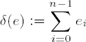
is the number of ones in the binary representation of e. If we assume that each digit takes on the value 0 or 1 with equal probability, then we may conclude that δ(e) has the expected value δ(e) = n/2, and altogether we have
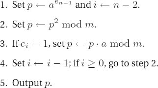
Binary algorithm for exponentiation of ae modulo m
The following implementation of this algorithm gives good results already for small exponents, those that can be represented by the USHORT type.
mixed modular exponentiation with | |
Syntax: | int umexp_l (CLINT bas_l, USHORT e, CLINT p_l,
CLINT m_l); |
Input: | bas_l (base) e (exponent) m_l (modulus) |
Output: |
|
Return: | E_CLINT_OK if all ok E_CLINT_DBZ if division by 0 |
int
umexp_l (CLINT bas_l, USHORT e, CLINT p_l, CLINT m_l)
{
 CLINT tmp_l, tmpbas_l;
 USHORT k = BASEDIV2;
 int err = E_CLINT_OK;
 if (EQZ_L (m_l))
  {
   return E_CLINT_DBZ;     /* division by zero */
  }
 if (EQONE_L (m_l))
  {
   SETZERO_L (p_l);        /* modulus = 1 ==> remainder = 0 */
   return E_CLINT_OK;
  }
 if (e == 0)     /* exponent = 0 ==> remainder = 1 */
  {
   SETONE_L (p_l);
   return E_CLINT_OK;
  }
 if (EQZ_L (bas_l))
  {
   SETZERO_L (p_l);
   return E_CLINT_OK;
  }
 mod_l (bas_l, m_l, tmp_l);
 cpy_l (tmpbas_l, tmp_l);
Note
After various checks the position of the leading 1 of the exponent e is determined. Here the variable k is used to mask the individual binary digits of e. Then k is shifted one more place to the right, corresponding to setting i ← n - 2 in step 1 of the algorithm.
while ((e & k) == 0)
 {
  k >>= 1;
 }
k >>= 1;
Note
For the remaining digits of e we run through steps 2 and 3. The mask k serves as loop counter, which we shift to the right one digit each time. We then multiply by the base reduced modulo m_l.
while (k != 0)
  {
   msqr_l (tmp_l, tmp_l, m_l);
   if (e & k)
    {
     mmul_l (tmp_l, tmpbas_l, tmp_l, m_l);
    }
   k >>= 1;
  }
 cpy_l (p_l, tmp_l);
 return err;
}
The binary algorithm for exponentiation offers particular advantages when it is used with small bases. If the base is of type USHORT, then all of the multiplications p ← pa mod m in step 3 of the binary algorithm are of the type CLINT * USHORT modulo CLINT, which makes possible a substantial increase in speed in comparison to other algorithms that in this case would also require the multiplication of two CLINT types. The squarings, to be sure, use CLINT objects, but here we are able to use the advantageous squaring function.
Thus in the following we shall implement the exponentiation function wmexp_l(), the dual to umexp_l(), which accepts a base of type USHORT. The masking out of bits of the exponent is a good preparatory exercise in view of the following "large" functions for exponentiation. The way of proceeding consists essentially in testing one after the other each digit ei of the exponent against a variable b initialized to 1 in the highest-valued bit, and then shifting to the right and repeating the test until b is equal to 0.
The following function wmexp_l() offers for small bases and exponents up to 1000 bits, for example, a speed advantage of about ten percent over the universal procedures that we shall tackle later.
Function: | modular exponentiation of a |
Syntax: | int wmexp_l (USHORT bas, CLINT e_l, CLINT rest_l,
CLINT m_l); |
Input: | bas (base) e_l (exponent) m_l (modulus) |
Output: | rest_l (remainder of base_l mod m_l) |
Return: | E_CLINT_OK if all is ok E_CLINT_DBZ if division by 0 |
int
wmexp_l (USHORT bas, CLINT e_l, CLINT rest_l, CLINT m_l)
{
 CLINT p_l, z_l;
 USHORT k, b, w;
 if (EQZ_L (m_l))
  {
   return E_CLINT_DBZ;     /* division by 0 */
  }
 if (EQONE_L (m_l))
  {
   SETZERO_L (rest_l);     /* modulus = 1 ==> remainder = 0 */
   return E_CLINT_OK;
  }
 if (EQZ_L (e_l))
  {
   SETONE_L (rest_l);
   return E_CLINT_OK;
  }
 if (0 == bas)
  {
   SETZERO_L (rest_l);
   return E_CLINT_OK;
  }
 SETONE_L (p_l);
 cpy_l (z_l, e_l);
Note
Beginning with the highest-valued nonzero bit in the highest-valued word of the exponent z_l the bits of the exponent are processed, where always we have first a squaring and then, if applicable, a multiplication. The bits of the exponent are tested in the expression if ((w & b) > 0) by masking their value with a bitwise AND.
b = 1 << ((ld_l (z_l) - 1) & (BITPERDGT - 1UL));
w = z_l[DIGITS_L (z_l)];
for (; b > 0; b >>= 1)
 {
  msqr_l (p_l, p_l, m_l);
  if ((w & b) > 0)
   {
    ummul_l (p_l, bas, p_l, m_l);
   }
 }
Note
Then follows the processing of the remaining digits of the exponent.
for (k = DIGITS_L (z_l) - 1; k > 0; k--)
 {
  w = z_l[k];
  for (b = BASEDIV2; b > 0; b >>= 1)
   {
    msqr_l (p_l, p_l, m_l);
    if ((w & b) > 0)
     {
      ummul_l (p_l, bas, p_l, m_l);
     }
    }
  }
 cpy_l (rest_l, p_l);
 return E_CLINT_OK;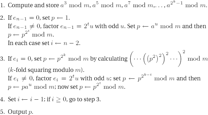
}Through a generalization of the binary algorithm on page 82 the number of modular multiplications for exponentiation can be reduced even further. The idea is to represent the exponent in a base greater than 2 and to replace multiplication by a in step 3 by multiplication by powers of a. Thus let the exponent e be given by
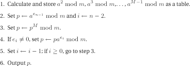
M-ary algorithm for exponentiation ae mod m
The number of necessary multiplications evidently depends on the number of digits of the exponent e and thus on the choice of M. Therefore, we would like to determine M such that the exponentiation in step 3 can be computed to the greatest extent possible by means of squaring, as in the example above for 216, and such that the number of multiplications by the precomputed powers of a be minimized to a justifiable cost of storage space for the table.
The first condition suggests that we choose M as a power of 2: M = 2k. In view of the second condition we consider the number of modular multiplications as a function of M:
We require
squares in step 3 and on average

modular multiplications in step 4, where
is the probability that a digit ei of e is nonzero. If we include the M - 2 multiplications for the computation of the table, then the M-ary algorithm requires on average
modular squarings and multiplications.
For exponents e and moduli m of, say, 512 binary places and M = 2k we obtain the numbers of modular multiplications for the calculation of ae mod m as shown in Table 6-1. The table shows as well the memory requirement for the precomputed powers of a mod m, which result from the product (2k - 2)CLINTMAXSHORT . sizeof(USHORT).
Table 6-1. Requirements for exponentiation
k | Multiplications | Memory (in Bytes) |
|---|---|---|
1 | 766 | 0 |
2 | 704 | 1028 |
3 | 666 | 3084 |
4 | 644 | 7196 |
5 | 640 | 15420 |
6 | 656 | 31868 |
We see from the table that the average number of multiplications reaches a minimum of 640 at k = 5, where the required memory for each larger k grows by approximately a factor of 2. But what are the time requirements for other orders of magnitude of the exponents?
Table 6.2 gives information about this. It displays the requirements for modular multiplication for exponentiation with exponents with various numbers of binary digits and various values of M = 2k. The exponent length of 768 digits was included because it is a frequently used key length for the RSA cryptosystem (see Chapter 17). The favorable numbers of multiplications appear in boldface.
Table 6-2. Numbers of multiplications for typical sizes of exponents and various bases 2k
Number of Binary Digits in the Exponent | |||||||||
|---|---|---|---|---|---|---|---|---|---|
k | 32 | 64 | 128 | 512 | 768 | 1024 | 2048 | 4096 | |
1 | 45 | 93 | 190 | 766 | 1150 | 1534 | 3070 | 6142 | |
2 | 44 | 88 | 176 | 704 | 1056 | 1408 | 2816 | 5632 | |
3 | 46 | 87 | 170 | 666 | 996 | 1327 | 2650 | 5295 | |
4 | 52 | 91 | 170 | 644 | 960 | 1276 | 2540 | 5068 | |
5 | 67 | 105 | 181 | 640 | 945 | 1251 | 2473 | 4918 | |
6 | 98 | 135 | 209 | 656 | 954 | 1252 | 2444 | 4828 | |
7 | 161 | 197 | 271 | 709 | 1001 | 1294 | 2463 | 4801 | |
8 | 288 | 324 | 396 | 828 | 1116 | 1404 | 2555 | 4858 |
In consideration of the ranges of numbers for which the FLINT/C package was developed, it appears that with k = 5 we have found the universal base M = 2k, with which, however, there is a rather high memory requirement of 15 kilobytes for the powers a2, a3, . . . , a31 to base a that are to be precomputed. The M-ary algorithm can be improved, however, according to [Cohe], Section 1.2, to the extent that we can employ not M - 2, but only M/2, premultiplications and thus require only half the memory. The task now additionally consists in the calculation of the power ae mod m, where
M-ary Algorithm for exponentiation with reduced number of premultiplications
The trick of this algorithm consists in dividing up the squarings required in step 3 in a clever way, such that the exponentiation of a is taken care of together with the even part 2t of ei. Within the squaring process the exponentiation of a by the odd part u of ei remains. The balance between multiplication and squaring is shifted to the more favorable squaring, and only the powers of a with odd exponent need to be precomputed and stored.
For this splitting one requires the uniquely determined representation ei = 2tu, u odd, of the exponent digit ei. For rapid access to t and u a table is used, which, for example, for k = 5 is displayed in Table 6-3.
To calculate these values we can use the auxiliary function twofact_l(), which will be introduced in Section 10.4.1. Before we can program the improved M-ary algorithm there remains one problem to be solved: How, beginning with the binary representation of the exponent or the representation to base B = 216, do we efficiently obtain its representation to base M = 2k for a variable k > 0? It will be of use here to do a bit of juggling with the various indices, and we can "mask out" the required digits ei to base M from the representation of e to base B. For this we set the following: Let
Let
With these settings the following statements hold:
There are f + 1 digits in
esi contains the least-significant bit of the digit e′i.
di specifies the position of the least-significant bit of e′i in esi (counting of positions begins with 0). If i < f and di > 16 - k, then not all the binary digits of e′i are in esi; the remaining (higher-valued) bits of e′i are in esi+1. The desired digit e′i thus corresponds to the k least-significant binary digits of
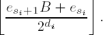
Table 6-3. Values for the factorization of the exponent digits into products of a power of 2 and an odd factor
ei | t | u | ei | t | u | ei | t | u |
|---|---|---|---|---|---|---|---|---|
0 | 0 | 0 | 11 | 0 | 11 | 22 | 1 | 11 |
1 | 0 | 1 | 12 | 2 | 3 | 23 | 0 | 23 |
2 | 1 | 1 | 13 | 0 | 13 | 24 | 3 | 3 |
3 | 0 | 3 | 14 | 1 | 7 | 25 | 0 | 25 |
4 | 2 | 1 | 15 | 0 | 15 | 26 | 1 | 13 |
5 | 0 | 5 | 16 | 4 | 1 | 27 | 0 | 27 |
6 | 1 | 3 | 17 | 0 | 17 | 28 | 2 | 7 |
7 | 0 | 7 | 18 | 1 | 9 | 29 | 0 | 29 |
8 | 3 | 1 | 19 | 0 | 19 | 30 | 1 | 15 |
9 | 0 | 9 | 20 | 2 | 5 | 31 | 0 | 31 |
10 | 1 | 5 | 21 | 0 | 21 |
As a result we have for
Since for the sake of simplicity we set e_l [sf + 2] ← 0, this expression holds as well for i = f.
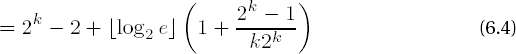
We have thus found an efficient method for accessing the digits of the exponent in its CLINT representation, which arise from its representation in a power-of-two base 2k with k ≤ 16, whereby we are saved an explicit transformation of the exponent. The number of necessary multiplications and squarings for the exponentiation is now
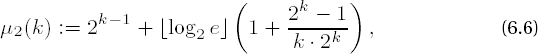
where in comparison to μ1(k) (see page 87) the expenditure for the precomputations has been reduced by half. The table for determining the favorable values of k (Table 6-4) now has a somewhat different appearance.
Table 6-4. Numbers of multiplications for typical sizes of exponents and various bases 2k
Number of Binary Digits in the Exponent | |||||||||
|---|---|---|---|---|---|---|---|---|---|
k | 32 | 64 | 128 | 512 | 768 | 1024 | 2048 | 4096 | |
1 | 47 | 95 | 191 | 767 | 1151 | 1535 | 3071 | 6143 | |
2 | 44 | 88 | 176 | 704 | 1056 | 1408 | 2816 | 5632 | |
3 | 44 | 85 | 168 | 664 | 994 | 1325 | 2648 | 5293 | |
4 | 46 | 85 | 164 | 638 | 954 | 1270 | 2534 | 5066 | |
5 | 53 | 91 | 167 | 626 | 931 | 1237 | 2459 | 4904 | |
6 | 68 | 105 | 179 | 626 | 924 | 1222 | 2414 | 4798 | |
7 | 99 | 135 | 209 | 647 | 939 | 1232 | 2401 | 4739 | |
8 | 162 | 198 | 270 | 702 | 990 | 1278 | 2429 | 4732 |
Starting with 768 binary digits of the exponent, the favorable values of k are larger by 1 than those given in the table for the previous version of the exponentiation algorithm, while the number of required modular multiplications has easily been reduced. It is to be expected that this procedure is on the whole more favorable than the variant considered previously. Nothing now stands in the way of an implementation of the algorithm.
To demonstrate the implementation of these principles we select an adaptive procedure that uses the appropriate optimal value for k. To accomplish this we rely again on [Cohe] and look for, as is specified there, the smallest integer value k that satisfies the inequality
which comes from the formula μ2(k) given previously for the number of necessary multiplications based on the condition μ2(k + 1) - μ2(k) ≥ 0. The constant number of modular squarings [log2 e] for all algorithms for exponentiation introduced thus far is eliminated; here only the "real" modular multiplications, that is, those that are not squarings, are considered.
The implementation of exponentiation with variable k requires a large amount of main memory for storing the precomputed powers of a; for k = 8 we require about 64 Kbyte for 127 CLINT variables (this is arrived at via (27 - 1) * sizeof(USHORT) * CLINTMAXSHORT)), where two additional automatic CLINT fields were not counted. For applications with processors or memory models with segmented 16-bit architecture this already has reached the limit of what is possible (see in this regard, for example, [Dunc], Chapter 12, or [Petz], Chapter 7).
Depending on the system platform there are thus various strategies appropriate for making memory available. While the necessary memory for the function mexp5_l() is taken from the stack (as automatic CLINT variables), with each call of the following function mexpk_l() memory is allocated from the heap. To save the expenditure associated with this, one may imagine a variant in which the maximum needed memory is reserved during a one-time initialization and is released only at the end of the entire program. In each case it is possible to fit memory management to the concrete requirements and to orient oneself to this in the commentaries on the following code.
One further note for applications: It is recommended always to check whether it suffices to employ the algorithm with the base M = 25. The savings in time that comes with larger values of k is relatively not so large in comparison to the total calculation time so as to justify in all cases the greater demand on memory and the thereby requisite memory management. Typical calculation times for various exponentiation algorithms, on the basis of which one can decide whether to use them, are given in Appendix D.
The algorithm, implemented with M = 25, is contained in the FLINT/C package as the function mexp5_l(). With the macro EXP_L() contained in flint.h one can set the exponentiation function to be used: mexp5_l() or the following function mexpk_l() with variable k.
modular exponentiation | |
Syntax: | int mexpk_l (CLINT bas_l, CLINT exp_l,
CLINT p_l, CLINT m_l); |
Input: | bas_l (base) exp_l (exponent) m_l (modulus) |
Output: |
|
Return: | E_CLINT_OK if all is ok E_CLINT_DBZ if division by 0 E_CLINT_MAL if malloc() error |
Note
We begin with a segment of the table for representing ei = 2tu, u odd, 0 ≤ ei < 28 The table is represented in the form of two vectors. The first, twotab[], contains the exponents t of the two-factor 2t, while the second, oddtab[], holds the odd part u of a digit 0 ≤ ei < 25. The complete table is contained, of course, in the FLINT/C source code.
static int twotab[] =
{0,0,1,0,2,0,1,0,3,0,1,0,2,0,1,0,4,0,1,0,2,0,1,0,3,0,1,0,2,0,1,0,5, ...};
static USHORT oddtab[]=
{0,1,1,3,1,5,3,7,1,9,5,11,3,13,7,15,1,17,9,19,5,21,11,23,3,25,13, ...};
int
mexpk_l (CLINT bas_l, CLINT exp_l, CLINT p_l, CLINT m_l)
{
Note
The definitions reserve memory for the exponents plus the leading zero, as well as a pointer clint **aptr_l to the memory still to be allocated, which will take pointers to the powers of bas_l to be precomputed. In acc_l the intermediate results of the exponentiation will be stored.
CLINT a_l, a2_l;
clint e_l[CLINTMAXSHORT + 1];
CLINTD acc_l;
clint **aptr_l, *ptr_l;
int noofdigits, s, t, i;
ULONG k;
unsigned int lge, bit, digit, fk, word, pow2k, k_mask;
Note
Then comes the usual checking for division by 0 and reduction by 1.
if (EQZ_L (m_l))
 {
  return E_CLINT_DBZ;
 }
if (EQONE_L (m_l))
 {
  SETZERO_L (p_l);    /* modulus = 1 ==> residue = 0 */
  return E_CLINT_OK;
 }
Note
Base and exponent are copied to the working variables a_l and e_l, and any leading zeros are purged.
cpy_l (a_l, bas_l);
cpy_l (e_l, exp_l);
Note
Now we process the simple cases a0 = 1 and 0e = 0 (e > 0).
if (EQZ_L (e_l))
 {
  SETONE_L (p_l);
  return E_CLINT_OK;
 }
if (EQZ_L (a_l))
 {
  SETZERO_L (p_l);
  return E_CLINT_OK;
 }
Note
Next, the optimal value for k is determined; the value 2k is stored in pow2k, and in k_mask the value 2k - 1. For this the function ld_l() is used, which returns the number of binary digits of its argument.
lge = ld_l (e_l);
k = 8;
while (k > 1 && ((k - 1) * (k << ((k - 1) << 1))/((1 << k ) - k - 1)) >= lge - 1)
 {
  --k;
 }
pow2k = 1U << k;
k_mask = pow2k - 1U;
Note
Memory is allocated for the pointers to the powers of a_l to be computed. The base a_l is reduced modulo m_l.
if ((aptr_l = (clint **) malloc (sizeof(clint *) * pow2k)) == NULL)
 {
  return E_CLINT_MAL;
 }
mod_l (a_l, m_l, a_l);
aptr_l[1] = a_l;
Note
If k > 1, then memory is allocated for the powers to be computed. This is not necessary for k = 1, since then no powers have to be precomputed. In the following setting of the pointer aptr_l[i] one should note that in the addition of an offset to a pointer p a scaling of the offset by the compiler takes place, so that it counts objects of the pointer type of p.
We have already mentioned that the allocation of working memory can be carried out alternatively in a one-time initialization. The pointers to the CLINT objects would in this case be contained in global variables outside of the function or in static variables within mexpk_l().
if (k > 1)
 {
  if ((ptr_l = (clint *) malloc (sizeof(CLINT) * ((pow2k >> 1) - 1))) == NULL)
   {
    return E_CLINT_MAL;
   }
  aptr_l[2] = a2_l;
  for (aptr_l[3] = ptr_l, i = 5; i < (int)pow2k; i+=2)
   {
    aptr_l[i] = aptr_l[i - 2] + CLINTMAXSHORT;
   }
Note
Now comes the precomputation of the powers of the value a stored in a_l. The values a3, a5, a7 , . . . , ak - 1 are computed (a2 is needed only in an auxiliary role).
msqr_l (a_l, aptr_l[2], m_l);
for (i = 3; i < (int)pow2k; i += 2)
 {
  mmul_l (aptr_l[2], aptr_l[i - 2], aptr_l[i], m_l);
 }
}
Note
This ends the case distinction for k > 1. The exponent is lengthened by the leading zero.
*(MSDPTR_L (e_l) + 1) = 0;
Note
The determination of the value f (represented by the variable noofdigits).
noofdigits = (lge - 1)/k;
fk = noofdigits * k;
Note
Word position si and bit position di of the digit ei in the variables word and bit.
word = fk >> LDBITPERDGT;     /* fk div 16 */
bit = fk & (BITPERDGT-1U);     /* fk mod 16 */
Note
Calculation of the digit en−1 with the above-derived formula; en−1 is represented by the variable digit.
switch (k)
 {
  case 1:
  case 2:
  case 4:
  case 8:
   digit = ((ULONG)(e_l[word + 1] ) >> bit) & k_mask;
   break;
  default:
   digit = ((ULONG)(e_l[word + 1] | ((ULONG)e_l[word + 2]
                                              << BITPERDGT)) >> bit) & k_mask;
}
Note
First run through step 2 of the algorithm, the case digit = en−1 ≠ 0.
if (digit != 0)    /* k-digit > 0 */
 {
  cpy_l (acc_l, aptr_l[oddtab[digit]]);
Note
Calculation of p2t; t is set to the two-part of en−1 via twotab[en−1]; p is represented by acc_l.
t = twotab[digit];
  for (; t > 0; t--)
   {
    msqr_l (acc_l, acc_l, m_l);
   }
  }
 else    /* k-digit == 0 */
  {
   SETONE_L (acc_l);
  }
Note
Loop over noofdigits beginning with f - 1.
for (--noofdigits, fk -= k; noofdigits >= 0; noofdigits--, fk -= k)
 {
Note
Word position si and bit position di of the digit ei in the variables word and bit.
word = fk >> LDBITPERDGT;   /* fk div 16 */
bit = fk & (BITPERDGT - 1U);         /* fk mod 16 */
Note
Computation of the digit ei with the formula derived above; ei is represented by the variable digit.
switch (k)
 {
  case 1:
  case 2:
  case 4:
  case 8:
   digit = ((ULONG)(e_l[word + 1] ) >> bit) & k_mask;
   break;
  default:
   digit = ((ULONG)(e_l[word + 1] | ((ULONG)e_l[word + 2]
                                                 << BITPERDGT)) >> bit) & k_mask;
 }
Note
Step 3 of the algorithm, the case digit = ei ≠ 0; t is set via the table twotab[ei] to the two-part of ei.
if (digit != 0)    /* k-digit > 0 */
 {
  t = twotab[digit];
Note
Calculation of p2k-t au in acc_l. Access to au with the odd part u of ei is via aptr_l [oddtab [ei]].
for (s = k - t; s > 0; s--)
 {
  msqr_l (acc_l, acc_l, m_l);
 }
mmul_l (acc_l, aptr_l[oddtab[digit]], acc_l, m_l);
Note
Calculation of p2t; p is still represented by acc_l.
for (; t > 0; t--)
  {
   msqr_l (acc_l, acc_l, m_l);
  }
 }
else /* k-digit == 0 */
 {
Note
Step 3 of the algorithm, case ei = 0: Calculate p2k.
for (s = k; s > 0; s--)
  {
   msqr_l (acc_l, acc_l, m_l);
  }
 }
}
Note
End of the loop; output of acc_l as power residue modulo m_l.
cpy_l (p_l, acc_l);
Note
At the end, allocated memory is released.
free (aptr_l);
 if (ptr_l != NULL) free (ptr_l);
 return E_CLINT_OK;
}
The various processes of M-ary exponentiation can be clarified with the help of a numerical example. To this end let us examine the calculation of the power 1234667 mod 18577, which will be carried out by the function mexpk_l() in the following steps:
The representation of the exponent e = 667 can be expressed to the base 2k with k = 2 (cf. the algorithm for M -ary exponentiation on page 89), whereby the exponent e has the representation e = (10 10 01 10 11)22.
The power a3 mod 18577 has the value 17354. Further powers of a do not arise in the precomputation because of the small size of the exponent.
Exponentiation loop
exponent digit ei = 2tu
21•1
21•1
20•1
21•1
20•3
p ← p2 mod n
-
14132
13261
17616
13599
p ← p22 mod n
-
-
4239
-
17343
p ← pau mod n
1234
13662
10789
3054
4445
p ← p2 mod n
18019
7125
-
1262
-
Result
p = 1234667 mod 18577 = 4445.
As an extension to the general case we shall introduce a special version of exponentiation with a power of two 2k as exponent. From the above considerations we know that this function can be implemented very easily by means of k-fold exponentiation. The exponent 2k will be specified by k.
Function: | modular exponentiation with exponent a power of 2 |
Syntax: | int mexp2_l (CLINT a_l, USHORT k, CLINT p_l,
CLINT m_l); |
Input: | a_l (base) k (exponent of 2) m_l (modulus) |
Output: |
|
Return: | E_CLINT_OK if all is ok E_CLINT_DBZ if division by 0 |
int
mexp2_l (CLINT a_l, USHORT k, CLINT p_l, CLINT m_l)
{
 CLINT tmp_l;
 if (EQZ_L (m_l))
  {
   return E_CLINT_DBZ;
  }
Note
If k > 0, then a_l is squared k times modulo m_l.
if (k > 0)
  {
   cpy_l (tmp_l, a_l);
   while (k-- > 0)
    {
     msqr_l (tmp_l, tmp_l, m_l);
    }
   cpy_l (p_l, tmp_l);
  }
else
Note
Otherwise, if k = 0, we need only to reduce modulo m_l.
{
   mod_l (a_l, m_l, p_l);
  }
 return E_CLINT_OK;
}A number of algorithms for exponentiation have been published, some of which are conceived for arbitrary operands and others for special cases. The goal is always to find procedures that employ as few multiplications and divisions as possible. The passage from binary to M-ary exponentiation is an example of how the number of these operations can be reduced.
Binary and M-ary exponentiation are themselves special cases of the construction of addition chains (cf. [Knut], Section 4.6.3). We have already taken advantage of the fact that the laws of exponentiation allow the additive decomposition of the exponent of a power:
from which follows the exponentiation in the form of alternating squarings and multiplications (cf. page 82):
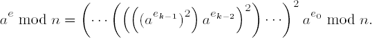
The associated addition chain is obtained by considering the exponents to powers of a that arise as intermediate results in this process:
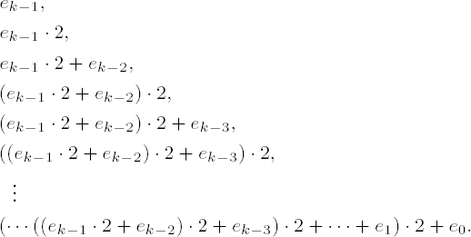
Here terms of the sequence are omitted if ej = 0 for a particular j. For the number 123, for example, based on the binary method the result is the following addition chain with 12 elements: 1, 2, 3, 6, 7, 14, 15, 30, 60, 61, 122, 123.
In general, a sequence of numbers 1 = a0, a1, a2, . . . , ar = e for which for every i = 1, . . . , r there exists a pair (j, k) with j ≤ k < i such that ai = aj + ak holds is called an addition chain for e of length r.
The M-ary method generalizes this principle for the representation of the exponent to other bases. Both methods have the goal of producing addition chains that are as short as possible, in order to minimize the calculational expense for the exponentiation. The addition chain for 123 produced by the 23-ary method is 1, 2, 3, 4, 7, 8, 15, 30, 60, 120, 123; with the 24-ary method the addition chain 1, 2, 3, 4, 7, 11, 14, 28, 56, 112, 123 is created. These last chains are, as expected, considerably shorter than those obtained by the binary method, which for larger numbers will have a greater effect than in this example. In view of the real savings in time one must, however, note that in the course of initialization for the calculation of ae mod n the M-ary methods construct the powers a2, a3, a5, aM−1 also for those exponents that are not needed in the representation of e to the base M or for the construction of the addition chain.
Binary exponentiation represents the worst case of an addition chain: By considering it we obtain a bound on the greatest possible length of an addition chain of log2 e + H (e) − 1, where H(e) denotes the Hamming weight of e.[14] The length of an addition chain is bounded below by log2 e + log2 H (e) − 2.13, and so a shorter addition chain for e is not to be found (cf. [Scho] or [Knut], Section 4.6.3, Exercises 28, 29). For our example this means that the shortest addition chain for e = 123 has length at least 8, and so the results of the M-ary methods cited earlier seem not to be the best possible.
The search for shortest addition chains is a problem for which there is as yet no known polynomial-time procedure. It lies in the complexity class NP of those decision problems that can be solved in polynomial time by nondeterministic methods, that is, those that can be solved by "guessing," where the necessary time for calculation is bounded by a polynomial p that is a function of the size of the input. In contrast to this, the class P contains those problems that can be solved deterministically in polynomial time.[15] It is not surprising that P is a subset of NP, since all polynomial-time deterministic problems can also be solved nondeterministically.
The determination of the shortest addition chain is an NP-complete problem, that is, a problem that is at least as difficult to solve as all other problems in the set NP (cf. [Yaco] and [HKW], page 302). The NP-complete problems are therefore of particular interest, since if for even one of them a deterministic polynomial-time procedure could be found, then all other problems in NP could be solved in polynomial time as well. In this case, the classes P and NP would collapse into a single set of problems. Although P ≠ NP is conjectured, this problem has remained unsolved, and it represents a central problem of complexity theory.
With this it is clear that all practical procedures for generating addition chains must rest on heuristics, that is to say, mathematical rules of thumb such as that for the determination of the exponent k in 2k-ary exponentiation, of which one knows that it has better time behavior than other methods.
For example, in 1990 Y. Yacobi [Yaco] described a connection between the construction of addition chains and the compression of data according to the Lempel–Ziv procedure; there an exponentiation algorithm based on this compression procedure as well as on the M-ary method is also given.
In the search for the shortest possible addition chains the M-ary exponentiation can be further generalized, which we shall pursue below in greater detail. The window methods represent the exponent not as in the M-ary method by digits to a fixed base M, but by digits of varying binary lengths. Thus, for example, long sequences of binary zeros, called zero windows, can appear as digits of the exponent. If we recall the M-ary algorithm from page 89, it is clear that for a zero window of length l only the l-fold repetition of squaring is required, and the corresponding step is then

Digits different from zero will be treated, depending on the process, either as windows of fixed length or as variable windows with a maximal length. As with the M-ary process, for every nonzero window (in the following called not quite aptly a "1-window") of length t, in addition to the repeated squaring an additional multiplication by a precalculated factor is required, in analogy to the corresponding step of the 2k-ary procedure:
The number of factors to be precomputed depends on the permitted maximal length of the 1-window. One should note that the 1-windows in the least-significant position always have a 1 and thus are always odd. The factorization of the exponent digit on page 89 into an even and odd factor will thus at first not be needed. On the other hand, in the course of exponentiation the exponent is processed from the most-significant to least-significant place, which means for the implementation that first the complete decomposition of the exponent must be carried out and stored before the actual exponentiation can take place.
Yet, if we begin the factorization of the exponent at the most-significant digit and travel from left to right, then every 0- or 1-window can be processed immediately, as soon as it is complete. This means, of course, that we will also obtain 1-windows with an even value, but the exponentiation algorithm is prepared for that.
Both directions of decomposition of the exponent into 1-windows with fixed length l follow essentially the same algorithm, which we formulate below for decomposition from right to left.
Decomposition of an integer e into 0-windows and 1-windows having fixed length l
If the least-significant binary digit is equal to 0, then begin a 0-window and go to step 2; otherwise, begin a 1-window and go to step 3.
Add the next-higher binary digits in a 0-window as long as no 1 appears. If a 1 appears, then close the 0-window, begin a 1-window, and go to step 3.
Collect a further l − 1 binary digits into a 1-window. If the next-higher digit is a 0, begin a 0-window and go to step 2; otherwise, begin a 1-window and go to step 3. If in the process all digits of e have been processed, then terminate the algorithm.
The decomposition from left to right begins with the most-significant binary digit and otherwise proceeds analogously. If we suppose that e has no leading binary zeros, then the algorithm cannot reach the end of the representation of e within step 2, and the procedure terminates in step 3 under the same condition given there. The following examples illustrate this process:
Let e = 1896837 = (111001111000110000101)2, and let l = 3. Beginning with the least-significant binary digit, e is decomposed as follows:
The choice l = 4 leads to the following decomposition of e:
The 2k-ary exponentiation considered above yields, for example for k = 2, the following decomposition:
The window decomposition of e for l = 3 contains five 1-windows, while that for l = 4 has only four, and for each the same number of additional multiplications is required. On the other hand, the 22-ary decomposition of e contains eight 1-windows, requires double the number of additional multiplications compared to the case l = 4, and is thus significantly less favorable.
The same procedure, but beginning with the most-significant binary digit, yields for l = 4 and e = 123 the decomposition
likewise with four 1-windows, which, as already established above, are not all odd.
Finally, then, exponentiation with a window decomposition of the exponent can be formalized by the following algorithm. Both directions of window decomposition are taken into account.
Algorithm for exponentiation ae mod m with the representation of e in windows of (maximal) length l for odd 1-windows
Decompose the exponent e into 0- and 1-windows (ωk−1 . . .ω0) of respective lengths lk−1, . . . ,l0.
Calculate and store a3 mod m, a5 mod m, a7 mod m, . . ., a2l−1 mod m.
Set p ← aωk−1 mod m and i ← k−2.
Set p ← pli mod m.
If ωi ≠ 0, set p ← paωi mod m.
Set i ← i - 1; if i ≥ 0, go to step 4.
Output p.
If not all 1-windows are odd, then steps 3 through 6 are replaced by the following, and there is no step 7:
3′. If ωk−1 = 0, set p ← p2lk−1 mod  |
4′. If ωi = 0, set p ← p2li mod  |
| If ω ≠ 0, factor ωi = 2tu with odd u; set p ← p2li−t mod m, and then p ← pau mod m; now set p ← p2t mod m. |
| 5′. Set i ← i − 1; if i ≥ 0, go to step 4′. |
| 6′. Output p. |
Now we are going to abandon addition chains and turn our attention to another idea, one that is interesting above all from the algebraic point of view. It makes it possible to replace multiplications modulo an odd number n by multiplications modulo a power of 2, that is, 2k, which requires no explicit division and is therefore more efficient than a reduction modulo an arbitrary number n. This useful method for modular reduction was published in 1985 by P. Montgomery [Mont] and since then has found wide practical application. It is based on the following observation.
Let n and r be relatively prime integers, and let r−1 be the multiplicative inverse of r modulo n; and likewise let n−1 be the multiplicative inverse of n modulo r; and furthermore, define n′ := -n−1 mod r and m := tn′ mod r. For integers t we then have
Note that on the left side of the congruence we have taken congruences modulo r and a division by r (note that t + mn ≡ 0 mod r, so the division has no remainder), but we have not taken congruences modulo n. By choosing r as a power of 2 in the form 2s we can reduce a number x modulo r simply by slicing off x at the sth bit (counting from the least-significant bit), and we can carry out the division of x by r by shifting x to the right by s bit positions. The left side of (6.8) thus requires significantly less computational expense than the right side, which is what gives the equation its charm. For the two required operations we can invoke the functions mod2_l() (cf. Section 4.3) and shift_l() (cf. Section 7.1).
This principle of carrying out reduction modulo n is called Montgomery reduction. Below, we shall institute Montgomery reduction for the express purpose of speeding up modular exponentiation significantly in comparison to our previous results. Since the procedure requires that n and r be relatively prime, we must take n to be odd. First we have to deal with a couple of considerations.
We can clarify the correctness of the previous congruence with the help of some simple checking. Let us replace m on the left-hand side of (6.8) by the expression tn′ mod r, which is (6.9), and further, replace tn′ mod r by tn′ − r
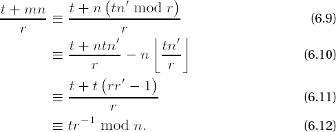
To summarize equation (6.8) we record the following: Let n, t, r €
we have
We shall return to this result later.
To apply Montgomery reduction we shift our calculations modulo n into a complete residue system (cf. Chapter 5)
with a suitable r := 2s>0 such that 2s−1 ≤ n < 2s. Then we define the Montgomery product "×" of two numbers a and b in R:
with r−1 representing the multiplicative inverse of r modulo n. We have
and thus the result of applying × to members of R is again in R. The Montgomery product is formed by applying Montgomery reduction, where again n′ := −n−1 mod r. From n′ we derive the representation 1 = gcd(n, r) = r′r − n′n, which we calculate in anticipation of Section 10.2 with the help of the extended Euclidean algorithm. From this representation of 1 we immediately obtain
1 ≡r′r mod n
and
1 ≡ −n′n mod r,
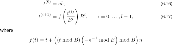
so that r′ = r−1 mod n is the multiplicative inverse of r modulo n, and n′ = −n−1 mod r the negative of the inverse of n modulo r (we are anticipating somewhat; cf. Section 10.2). The calculation of the Montgomery product now takes place according to the following algorithm.
Calculation of the Montgomery product a × b in R(r, n)
Set t ← ab.
Set m ← tn′ mod r.
Set u ← (t + mn)/r (the quotient is an integer; see above).
If u ≥ n, output u − n, and otherwise u. Based on the above selection of the parameter we have a, b < n as well as m, n < r and finally u < 2n; cf. (6.21).
The Montgomery product requires three long-integer multiplications, one in step 1 and two for the reduction in steps 2 and 3. An example with small numbers will clarify the situation: Let a = 386, b = 257, and n = 533. Further, let r = 210. Then n′ = −n−1 mod r = 707, m = 6, t + mn = 102400, and u = 100.
A modular multiplication ab mod n with odd n can now be carried out by first transforming a′ ← ar mod n and b′ ← br mod n to R, there forming the Montgomery product p′ ← a′ × b′ = a′b′r−1 mod n and then with p ← p′ × 1 = p′r−1 = ab mod n obtaining the desired result. However, we can spare ourselves the reverse transformation effected in the last step by setting p ← a′ × b at once and thus avoid the transformation of b, so that in the end we have the following algorithm.
Calculation of p = ab mod n (n odd) with the Montgomery product
Determine r := 2s with 2s−1 ≤ n < 2s. Calculate 1 = r′r − n′n by means of the extended Euclidean algorithm.
Set a′ ← ar mod n.
Set p ← a′ × b and output p.
Again we present an example with small numbers for clarification: Let a = 123, b = 456, n = 789, r = 210. Then n′ = −n−1 mod r = 963, a′ = 501, and p = a′ × b = 69 = ab mod n.
Since the precalculation of r′ and n′ in steps 1 and 2 is very time-consuming and Montgomery reduction in this version also has two long-number multiplications on its balance sheet, there is actually an increased computational expenditure compared with "normal" modular multiplication, so that the computation of individual products with Montgomery reduction is not worthwhile.
However, in cases where many modular multiplications with a constant modulus are required, for which therefore the time-consuming precalculations occur only once, we may expect more favorable results. Particularly suited for the Montgomery product is modular exponentiation, for which we shall suitably modify the M-ary algorithm. To this end let once again e = (em−1em−2 . . . e0)B and n = (nl−1nl−2 . . . n0)B be the representations of the exponent e and the modulus n to the base B = 2k. The following algorithm calculates powers ae mod n in • n with odd n using Montgomery multiplication. The squarings that occur in the exponentiation become Montgomery products a × a, in the computation of which we can use the advantages of squaring.
Exponentiation modulo n (n odd) with the Montgomery product
Set r ← Bl = 2kl. Calculate 1 = rr′ − nn′ with the Euclidean algorithm.
Set

If em−1 ≠ 0, factor em−1 = 2tu with odd u. Set
If em−1 = 0, set

In each case set i ← m − 2.
If ei = 0, set

If ei ≠ 0 factor ei = 2tu with odd u. Set

If i ≥ 0, set i ← i − 1 and go to step 4.
Output the Montgomery product

Further possibilities for improving the algorithm lie less in the exponentiation algorithm than in the implementation of the Montgomery product itself, as demonstrated by S. R. Dussé and B. S. Kaliski in [DuKa]: In calculating the Montgomery product on page 108, in step 2 we can avoid the assignment m ← tn′ mod r in the reduction modulo r. Furthermore, we can calculate with n′0 := n′ mod B instead of with n′ in executing the Montgomery reduction.
We can create a digit mi ← tin′0 modulo B, multiply it by n, scale by the factor Bi, and add to t. To calculate ab mod n with a, b < n the modulus n has the representation n = (nl−1nl−2 . . . n0)B as above, and we let r := Bl as well as rr′ − nn′ = 1 and n′0 := n′ mod B.
Calculation of the Montgomery product a × b à la Dussé and Kaliski
Set t ← ab, n′0 ← n′ mod B, i ← 0.
Set mi ← tin′0 mod B (mi is a one-digit integer).
Set t ← t + minBi.
Set i ← i + 1; if i ≤ l − 1, go to step 2.
Set t ←t/r.
If t ≥ n, output t − n and otherwise t.
Dussé and Kaliski state that the basis for their clever simplification is the method of Montgomery reduction to develop t as a multiple of r, but they offer no proof. Before we use this procedure we wish to make more precise why it suffices to calculate a × b. The following is based on a proof of Christoph Burnikel [Zieg]:
| In steps 2 and 3 the algorithm calculates a sequence |
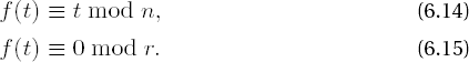
where
is the already familiar function that is induced by the Montgomery equation (cf. (6.13), and there set r ← B in f(t)). The members of the sequence t(i) have the properties
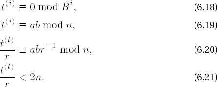
Properties (6.18) and (6.19) are derived inductively from (6.14), (6.15), (6.16), and (6.17); from (6.18) we obtain
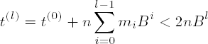
(note here that t(0) = ab < n2 < nBl).
The expenditure for the reduction is now determined essentially by multiplication of numbers of order of magnitude the size of the modulus. This variant of Montgomery multiplication can be elegantly implemented in code that forms the core of the multiplication routine mul_l() (cf. page 36).
Function: | Montgomery product |
Syntax: | void mulmon_l (CLINT a_l, CLINT b_l, CLINT n_l,
USHORT nprime, USHORT logB_r,
CLINT p_l); |
Input: | a_l, b_l (factors a and b) n_l (modulus n > a, b) nprime (n′ mod B) logB_r (logarithm of r to base B = 216; it must hold that BlogB_r−1 ≤ n < BlogB_r) |
Output: | p_l (Montgomery product a × b = a•b•r−1 mod n) |
void
mulmon_l (CLINT a_l, CLINT b_l, CLINT n_l, USHORT nprime,
         USHORT logB_r, CLINT p_l)
{
 CLINTD t_l;
 clint *tptr_l, *nptr_l, *tiptr_l, *lasttnptr, *lastnptr;
 ULONG carry;
 USHORT mi;
 int i;

 mult (a_l, b_l, t_l);
 lasttnptr = t_l + DIGITS_L (n_l);
 lastnptr = MSDPTR_L (n_l);
Note
The earlier use of mult() makes possible the multiplication of a_l and b_l without the possibility of overflow (see page 72); for the Montgomery squaring we simply insert sqr(). The result has sufficient space in t_l. Then t_l is given leading zeros to bring it to double the number of digits of n_l if t_l is smaller than this.
for (i = DIGITS_L (t_l) + 1; i <= (DIGITS_L (n_l) << 1); i++)
 {
  t_l[i] = 0;
 }
SETDIGITS_L (t_l, MAX (DIGITS_L (t_l), DIGITS_L (n_l) << 1));
Note
Within the following double loop the partial products minBi with mi := tin′0 are calculated one after the other and added to t_l. Here again the code is essentially that of our multiplication function.
for (tptr_l = LSDPTR_L (t_l); tptr_l <= lasttnptr; tptr_l++)
 {
  carry = 0;
  mi = (USHORT)((ULONG)nprime * (ULONG)*tptr_l);

  for (nptr_l = LSDPTR_L (n_l), tiptr_l = tptr_l;
    nptr_l <= lastnptr; nptr_l++, tiptr_l++)
   {
    *tiptr_l = (USHORT)(carry = (ULONG)mi * (ULONG)*nptr_l +
      (ULONG)*tiptr_l + (ULONG)(USHORT)(carry >> BITPERDGT));
   }
Note
In the following inner loop a possible overflow is transported to the most-significant digit of t_l, and t_l contains an additional digit in case it is needed. This step is essential, since at the start of the main loop t_l was given a value and not initialized via multiplication by 0 as was the variable p_l.
for ( ;
  ((carry >> BITPERDGT) > 0) && tiptr_l <= MSDPTR_L (t_l);
  tiptr_l++)
 {
  *tiptr_l = (USHORT)(carry = (ULONG)*tiptr_l +
                      (ULONG)(USHORT)(carry >> BITPERDGT));
 }
if (((carry >> BITPERDGT) > 0))
 {
  *tiptr_l = (USHORT)(carry >> BITPERDGT);
  INCDIGITS_L (t_l);
 }
}
Note
Now follows division by Bl, and we shift t_l by logB_r digits to the right, or ignore the logB_r least-significant digits of t_l. Then if applicable the modulus n_l is subtracted from t_l before t_l is returned as result into p_l.
tptr_l = t_l + (logB_r);
SETDIGIT_L (tptr_l, DIGITS_L (t_l) - (logB_r));
if (GE_L (tptr_l, n_l))
 {
  sub_l (tptr_l, n_l, p_l);
 }
else
 {
  cpy_l (p_l, tptr_l);
 }
}
The Montgomery squaring sqrmon_l() differs from this function only marginally: There is no parameter b_l in the function call, and instead of multiplication with mult(a_l, b_l, t_l) we employ the squaring function sqr(a_l, t_l), which likewise ignores a possible overflow. However, in modular squaring in the Montgomery method one must note that after the calculation of p′ ← a′ × a′ the reverse transformation p ← p′ × 1 = p′ r− 1 = a2 mod n must be calculated explicitly (cf. page 108).
Function: | Montgomery square |
Syntax: | void sqrmon_l (CLINT a_l, CLINT n_l, USHORT nprime,
USHORT logB_r, CLINT p_l); |
Input: | a_l (factor |
Output: | p_l (Montgomery square |
In their article Dussé and Kaliski also present the following variant of the extended Euclidean algorithm, to be dealt with in detail in Section 10.2, for calculating n′0 = n′ mod B, with which the expenditure for the precalculations can be reduced. The algorithm calculates −n−1 mod 2s for an s > 0 and for this requires long-number arithmetic.
Algorithm for calculating the inverse −n−1 mod 2s for s > 0, n odd
Set x ← 2, y ← 1, and i ← 2.
If x < ny mod x, set y ← y + x.
Set x ← 2x and i ← i + 1; if i ≤ s, go to step 2.
Output x − y.
With complete induction it can be shown that in step 2 of this algorithm yn ≡ 1 mod x always holds, and thus y ≡ n−1 mod x. After x has taken on the value 2s in step 3, we obtain with 2s − y ≡ −n−1 mod 2s the desired result if we choose s such that 2s ≡ B. The short function for this can be obtained under the name invmon_l() in the FLINT/C source. It takes only the modulus n as argument and outputs the value −n−1 mod B.
These considerations are borne out in the creation of the functions mexp5m_l() and mexpkm_l(), for which we give here only the interface, together with a computational example.
Function: | modular exponentiation with odd modulus(25 -ary or 2k -ary method with Montgomery product) |
Syntax: | int mexp5m_l (CLINT bas_l, CLINT exp_l,
CLINT p_l, CLINT m_l);
int mexpkm_l (CLINT bas_l, CLINT exp_l,
CLINT p_l, CLINT m_l); |
Input: | bas_l (base) exp_l (exponent) m_l (modulus) |
Output: |
|
Return: | E_CLINT_OK if all is ok E_CLINT_DBZ if division by 0 E_CLINT_MAL if malloc() error E_CLINT_MOD if even modulus |
These functions employ the routines invmon_l(), mulmon_l(), and sqrmon_l() to compute the Montgomery products. Their implementation is based on the functions mexp5_l() and mexpk_l() modified according to the exponentiation algorithm described above.
We would like to reconstruct the processes of Montgomery exponentiation in mexpkm_l() with the same numerical example that we looked at for M -ary exponentiation (cf. page 100). In the following steps we shall calculate the power 1234667 mod 18577:
Precomputations
The exponent e = 667 is represented to the base 2k with k = 2 (cf. the algorithm for Montgomery exponentiation on page 114). The exponent e thereby has the representation
The value r for Montgomery reduction is r = 216 = B = 65536.
The value n′0 (cf. page 110) is now calculated as n′0 = 34703.
The transformation of the base a into the residue system R(r, n) (cf. page 107) follows from
The power ā3 in R(r, n) has the value ā3 = 9227. Because of the small exponent, further powers of ā do not arise in the precomputation.
Exponentiation loop
exponent digit ei = 2tu
21 • 1
21 • 1
20 • 1
21 • 1
20 • 3

–
16994
3682
14511
11066

–
–
6646
–
12834

5743
15740
8707
16923
1583

9025
11105
–
1628
–
Result
The value of the power p after normalization:
Those interested in reconstructing the coding details of the functions mexp5m_l() and mexpkm_l() and the calculational steps of the example related to the function mexpkm_l() are referred to the FLINT/C source code.
At the start of this chapter we developed the function wmexp_l(), which has the advantage for small bases that only multiplications p ← pa mod m of the type CLINT * USHORT mod CLINT occur. In order to profit from the Montgomery procedure in this function, too, we adjust the modular squaring to Montgomery squaring, as in mexpkm_l(), with the use of the fast inverse function invmon_l(), though we leave the multiplication unchanged. We can do this because with the calculational steps for Montgomery squaring and for conventional multiplication modulo n,
we do not abandon the residue system R(r, n) = {ir mod n | 0 ≤ i < n } introduced above. This process yields us both the function wmexpm_l() and the dual function umexpm_l() for USHORT exponents, respectively for odd moduli, which in comparison to the two conventional functions wmexp_l() and umexp_l() again yields a significant speed advantage. For these functions, too, we present here only the interface and a numerical example. The reader is again referred to the FLINT/C source for details.
Function: | modular exponentiation with Montgomery reduction for USHORT-base, respectively |
Syntax: | int wmexpm_l (USHORT bas, CLINT e_l,
CLINT p_l, CLINT m_l);
int umexpm_l (CLINT bas_l, USHORT e,
CLINT p_l, CLINT m_l); |
Input: | bas, bas_l (base) e, e_l (exponent) m_l (modulus) |
Output: | p_l (residue of base_l mod m_l, resp. bas_le mod m_l) |
Return: | E_CLINT_OK if all is ok E_CLINT_DBZ if division by 0 E_CLINT_MOD if even modulus |
The function wmexpm_l() is tailor-made for our primality test in Section 10.5, where we shall profit from our present efforts. The function will be documented with the example used previously of the calculation of 1234667 mod 18577.
Precalculations
The binary representation of the exponent is e = (1010011011)2.
The value r for the Montgomery reduction is r = 216 = B = 65536.
The value n′0 (cf. page 110) is calculated as above, yielding n′0 = 34703.
The initial value of

Exponentiation loop
Exponent bit
1
0
1
0
0
1
1
0
1
1

9805
9025
16994
11105
3682
6646
14511
1628
11066
9350

5743
–
15740
–
–
8707
16923
–
1349
1583
Result
The value of the exponent p after normalization:
A detailed analysis of the time behavior of Montgomery reduction with the various optimizations taken into account can be found in [Boss]. There we are promised a ten to twenty percent saving in time over modular exponentiation by using Montgomery multiplication. As can be seen in the overviews in Appendix D of typical calculation times for FLINT/C functions, our implementations bear out this claim fully. To be sure, we have the restriction that the exponentiation functions that use Montgomery reduction can be used only for odd moduli. Nonetheless, for many applications, for example for encryption and decryption, as well as for computing digital signatures according to the RSA procedure (see Chapter 17), the functions mexp5m_l() and mexpkm_l() are the functions of choice.
Altogether, we have at our disposal a number of capable functions for modular exponentiation. To obtain an overview, in Table 6-5 we collect these functions together with their particular properties and domains of application.
Table 6-5. Exponentiation functions in FLINT/C
Function: | Domain of Application |
|---|---|
| General 25-ary exponentiation, without memory allocation, greater stack requirements. |
| General 2k -ary exponentiation with optimal k for |
| 25 -ary Montgomery exponentiation for odd moduli, without memory allocation, greater stack requirements. |
| 2k -ary Montgomery exponentiation for odd moduli, with optimal k for |
| Mixed binary exponentiation of a |
| Mixed binary exponentiation of a |
| Mixed binary exponentiation of a |
| Mixed binary exponentiation with Montgomery squaring of a |
| Mixed exponentiation with a power-of-2 exponent, lower stack requirements. |
We have worked hard in this chapter in our calculation of powers, and it is reasonable to ask at this point what modular exponentiation might have to offer to cryptographic applications. The first example to come to mind is, of course, the RSA procedure, which requires a modular exponentiation for encryption and decryption—assuming suitable keys. However, the author would like to ask his readers for a bit (or perhaps even a byte) of patience, since for the RSA procedure we still must collect a few more items, which we do in the next chapter. We shall return to this extensively in Chapter 17.
For those incapable of waiting, we offer as examples of the application of exponentiation two important algorithms, namely, the procedure suggested in 1976 by Martin E. Hellman and Whitfield Diffie [Diff] for the exchange of cryptographic keys and the encryption procedure of Taher ElGamal as an extension of the Diffie–Hellman procedure.
The Diffie–Hellman procedure represents a cryptographic breakthrough, namely, the first public key, or asymmetric, cryptosystem (see Chapter 17). Two years after its publication, Rivest, Shamir, and Adleman published the RSA procedure (see [Rive]). Variants of the Diffie–Hellman procedure are used today for key distribution in the Internet communications and security protocols IPSec, IPv6, and SSL, which were developed to provide security in the transfer of data packets in the IP protocol layer and the transfer of data at the application level, for example from the realms of electronic commerce. This principle of key distribution thus has a practical significance that would be difficult to overestimate.[16]
With the aid of the Diffie–Hellman protocol two communicators, Ms. A and Mr. B, say, can negotiate in a simple way a secret key that then can be used for the encryption of communications between the two. After A and B have agreed on a large prime number p and a primitive root a modulo p (we shall return to this below), the Diffie–Hellman protocol runs as follows.
Protocol for key exchange à la Diffie–Hellman
Since
after step 4, A and B are dealing with a common key. The values p and a do not have to be kept secret, nor the values yA and yB exchanged in steps 1 and 2. The security of the procedure depends on the difficulty in calculating discrete logarithms in finite fields, and the difficulty of breaking the system is equivalent to that of calculating values xA or xB from values yA or yB in • p.[17] That the calculation of axy from ax and ay in a finite cyclic group (the Diffie–Hellman problem) is just as difficult as the calculation of discrete logarithms and thus equivalent to this problem is, in fact, conjectured but has not been proved.
To ensure the security of the procedure under these conditions the modulus p must be chosen sufficiently large (at least 1024 bits, better 2048 or more; see Table 17-1), and one should ensure that p − 1 contains a large prime divisor close to (p − 1)/2 to exclude particular calculational procedures for discrete logarithms (a constructive procedure for such prime numbers will be presented in Chapter 17 in connection with the generation of strong primes, for example for the RSA procedure).
The procedure has the advantage that secret keys can be generated as needed on an ad hoc basis, without the need for secret information to be held for a long time. Furthermore, for the procedure to be used there are no further infrastructure elements necessary for agreeing on the parameters a and b. Nonetheless, this protocol possesses some negative characteristics, the gravest of which is the lack of authentication proofs for the exchanged parameters yA and yB. This makes the procedure susceptible to man-in-the-middle attacks, whereby attacker X intercepts the messages of A and B with their public keys yA and yB and replaces them with falsified messages to A and B containing his own public key yX.
Then A and B calculate "secret" keys s′A := yXxA mod p and s′B := yXxB mod p, which X on his or her part calculates s′A from yAxA ≡ axAxX ≡ axXxA ≡ yXxA ≡ s′A mod p and s′B analogously. The Diffie–Hellman protocal has now been executed not between A and B, but between X and A as well as between X and B. Now X is in a position to decode messages from A or B and to replace them by falsified messages to A or B. What is fatal is that from a cryptographic point of view the participants A and B are clueless as to what has happened.
To compensate for these defects without giving up the advantages, several variants and extensions have been developed for use in the Internet. They all take into account the necessity that key information be exchanged in such a way that its authenticity can be verified. This can be achieved, for example, by the public keys being digitally signed by the participants and the associated certificate of a certification authority being sent with them (see in this regard page 400, Section 17.3), which is implemented, for example, in the SSL protocol. IPSec and IPv6 use a complexly constructed procedure with the name ISAKMP/Oakley,[18] which overcomes all the drawbacks of the Diffie–Hellman protocol (for details see [Stal], pages 422–423).
To determine a primitive root modulo p, that is, a value a whose powers ai mod p with i = 0, 1, ... , p − 2 constitute the entire set of elements of the multiplicative group • pX = {1, ... , p − 1 } (see in this regard Section 10.2), the following algorithm can be used (see [Knut], Section 3.2.1.2, Theorem C). It is assumed that the prime factorization p − 1 = P1e1 . . . pekk of the order of
Finding a primitive root modulo p
Choose a random integer a € [0, p − 1] and set i ← 1.
Compute t ← a(p−1)/pi mod p.
If t = 1, go to step 1. Otherwise, set i ← i + 1. If i ≤ k, go to step 2. If i > k, output a and terminate the algorithm.
The algorithm is implemented in the following function.
Function: | ad hoc generation of a primitive root modulo p (2 < p prime) |
Syntax: | int primroot_l (CLINT a_l, unsigned noofprimes,
clint **primes_l); |
Input: |
|
Output: |
|
Return: |
− 1 if p − 1 odd and thus p is not prime |
int
primroot_l (CLINT a_l, unsigned int noofprimes, clint *primes_l[])
{
 CLINT p_l, t_l, junk_l;
 ULONG i;

 if (ISODD_L (primes_l[0]))
  {
   return −1;
  }
Note
primes_l[0] contains p − 1, from which we obtain the modulus in p_l.
cpy_l (p_l, primes_l[0]);
inc_l (p_l);
SETONE_L (a_l);

do
 {
  inc_l (a_l);
Note
As candidates a for the sought-after primitive root only natural numbers greater than or equal to 2 are tested. If a is a square, then a cannot be a primitive root modulo p, since then already a(p−1)/2 ≡ 1 mod p, and the order of a must be less than
if (issqr_l (a_l, t_l))
 {
  inc_l (a_l);
 }

i = 1;
Note
The calculation of t ← a(p − 1)/pi mod p takes place in two steps. All prime factors pi are tested in turn; we use Montgomery exponentiation. If a primitive root is found, it is output in a_l.
do
 {
  div_l (primes_l[0], primes_l[i++], t_l, junk_l);
  mexpkm_l (a_l, t_l, t_l, p_l);
 }
while ((i <= noofprimes) && !EQONE_L (t_l)); } while (EQONE_L (t_l)); return E_CLINT_OK; }
As a second example for the application of exponentiation we consider the encryption procedure of ElGamal, which as an extension of the Diffie–Hellman procedure also provides security in the matter of the difficulty of computing discrete logarithms, since breaking the procedure is equivalent to solving the Diffie–Hellman problem (cf. page 119). Pretty good privacy (PGP), the workhorse known throughout the world for encrypting and signing e-mail and documents whose development goes back essentially to the work of Phil Zimmermann, uses the ElGamal procedure for key management (see [Stal], Section 12.1).
A participant A selects a public and associated private key as follows.
ElGamal key generation
Achooses a large prime number p such that p − 1 has a large prime divisor close to (p − 1)/2 (cf. page 388) and a primitive root a of the multiplicative group
Achooses a random number x with 1 ≤ x > p − 1 and computes b := ax mod p with the aid of Montgomery exponentiation.As public key A uses the triple

Using the public key triple
Protocol for encryption à la ElGamal
Bchooses a random number y with 1 ≤ y < p − 1.Bcalculates α := ay mod p and β := Mby mod p = M (ax)y mod p.Bsends the cryptogram C := (α, β) toA.Acomputes from C the plain text using M = β/αx modulo p.
Since
the procedure works. The calculation of β/αx is carried out by means of a multiplication βαp−1−x modulo p.
The size of p should be, depending on the application, 1024 bits or longer (see Table 17-1), and for the encryption of different messages M1 and M2 unequal random values y1 ≠ y2 should be chosen, since otherwise, from
it would follow that knowledge of M1 was equivalent to knowledge of M2. In view of the practicability of the procedure one should note that the cryptogram C is twice the size of the plain text M, which means that this procedure has a higher transmission cost than others.
The procedure of ElGamal in the form we have presented has an interesting weak point, which is that an attacker can obtain knowledge of the plain text with a small amount of information. We observe that the cyclic group
axy €
U (ax € U or ay € U). This, and whether also β € U, is tested withFor all u €

One may ask how bad it might be if an attacker could gain such information about M. From the point of view of cryptography it is a situation difficult to accept, since the message space to be searched is reduced by half with little effort. Whether in practice this is acceptable certainly depends on the application. Surely, it is a valid reason to be generous in choosing the length of a key.
Furthermore, one can take some action against the weakness of the procedure, without, one hopes, introducing new, unknown, weaknesses: The multiplication Mby mod p in step 2 of the algorithm can be replaced with an encryption operation V (H (axy) , M) using a suitable symmetric encryption procedure V (such as Triple-DES, IDEA, or Rijndael, which has become the new advanced encryption standard; cf. Chapter 11) and a hash function H (cf. page 398) that so condenses the value axy that it can be used as a key for V.
So much for our examples of the application of modular exponentiation. In number theory, and therefore in cryptography as well, modular exponentiation is a standard operation, and we shall meet it repeatedly later on, in particular in Chapters 10 and 17. Furthermore, refer to the descriptions and numerous applications in [Schr] as well as in the encyclopedic works [Schn] and [MOV].
[14] If n possesses a representation n = (nk−1nk−2 . . . n0)2, then H(n) is defined as Σini (See [HeQu], Chapter 8.)
[15] If the input to such a problem is an integer n, then the number of digits of n can serve as a measure of the size of the input. There then exists a polynomial p such that the calculation time is bounded by p(log2 n). The difference whether the cost of solving the problem grows with n or with the number of digits of n is decisive.
[16] IP Security (IPSec), developed by the Internet Engineering Task Force (IETF), is, as an extensive security protocol, a part of the future Internet protocol IPv6. It was created so that it could also be used in the framework of the then current Internet protocol (IPv4). Secure Socket Layer (SSL) is a security protocol developed by Netscape that lies above the TCP protocol, which offers end-to-end security for applications such as HTTP, FTP, and SMTP (for all of this see [Stal], Chapters 13 and 14).
[17] For the problem of calculating discrete logarithms see [Schn], Section 11.6, as well as [Odly].
[18] ISAKMP: Internet Security Association and Key management Protocol.