
Constructing Spline Curves
A spline is a flexible rod of wood or plastic. It has its origins in shipbuilding, where splines were used to draft the curves (ribs) that define a ship body. Early uses go back to the 1600s, and are documented in [450]. Although mechanical splines are used less frequently now, the underlying principle still gives rise to new algorithms.
9.1 Greville Interpolation
In Chapter 7, we saw how to pass a polynomial curve of degree n through n + 1 data points p0, …, pn with parameter values t0, …, tn. The key to the solvability of the problem was simple: the number of knowns (the data points with parameter values) had to equal the number of unknowns (the polynomial coefficients).
Something quite analogous happens in a spline context. A spline curve of degree n is defined over a knot sequence u0, …, uK. Such a knot sequence has K – n + 2 Greville abscissae ξi and hence the spline curve has L + 1 = K – n + 2 B-spline control points d0, …, dL.
In view of these numbers, the following is a meaningful interpolation problem:
Given: A knot sequence u0, …, uK and a degree n, also a set of data points ![]() with
with ![]()
Find: A set of B-spline control points d0, …, dLuch that the resulting curve x(u) satisfies
In this case, the parameter values associated with the data points are not the knots ui but rather the Greville abscissae ξi. This gives us a problem in which the number of unknowns equals the number of knowns.
The solution is obtained in complete analogy to the polynomial case: write out (9.1) as

and collect them in matrix form:
There is a significant difference to the polynomial case: the matrix in (9.3) has nonzero entries only near the diagonal. Because of the local support property of B-splines, most of the ![]() are zero; at most n + 1 of them are nonzero for any
are zero; at most n + 1 of them are nonzero for any ![]() . This means that the matrix in (9.3) is banded and thus much easier to handle than a full matrix as encountered in polynomial interpolation. The cubic case (with triple end knots and simple interior knots) looks like this:
. This means that the matrix in (9.3) is banded and thus much easier to handle than a full matrix as encountered in polynomial interpolation. The cubic case (with triple end knots and simple interior knots) looks like this:
The ![]() elements represent the nonzero
elements represent the nonzero ![]() ; zero matrix entries are left blank. Instead of employing a general-purpose linear system solver, routines for banded matrices may be used—they are much more efficient.
; zero matrix entries are left blank. Instead of employing a general-purpose linear system solver, routines for banded matrices may be used—they are much more efficient.
Greville interpolation works well where the given data points correspond to the Greville abscissae of a knot sequence. It is the most commonly used method for quadratic spline interpolation; see [138] and [156].
In most practical situations, however, it will be hard to come up with such a knot sequence, and different methods are employed.
9.2 Least Squares Approximation
Curves are not always required to pass through a set of points; sometimes it may suffice to be close to the given points. In this case, we speak of approximating curves. We encountered situations like this in Section 7.8.
As an example, consider the generation of an airplane wing: its cross sections (profiles) are defined by analytical means, optimizing some airflow characteristics for example.1 One can now compute many (100, say) points on the profile and then ask for a curve through them. A cubic spline interpolant would do the job, but it would have too many segments—for a typical profile, a curve with 15 segments might provide a perfect fit. One possibility is to simply discard data points until we are left with the desired number. We would then compute the interpolant to the reduced data set and check if the discarded points are within tolerance. This is expensive, and a more frequently encountered approach is one that makes sure that all data points are as close as possible to the curve, avoiding any iterations.
To make matters more precise, assume that we are given data points pi with i = 0, …, P.2 We wish to find an approximating B-spline curve p(u) of degree n with K + 1 knots u0, …, uK. We want the curve to be close to the data points in the least squares sense. Suppose the data point pi is associated with a data parameter value wi.3 Then we would like the distance ![]() pi – p(wi)
pi – p(wi)![]() to be small. Attempting to minimize all such distances then amounts to
to be small. Attempting to minimize all such distances then amounts to
The squared distances are introduced to simplify our subsequent computations. They gave the name to this method: least squares approximation. We shall minimize (9.5) by finding suitable B-spline control vertices dj:
The least squares approach—identical to our development of the polynomial case in Section 7.8—produces the normal equations

This is a linear system of L + 1 equations for the unknowns dk, with a coefficient matrix M whose elements mj,k are given by
The symmetric matrix M is often ill conditioned—special equation solvers, such as a Cholesky decomposition, should be employed. For more details on the numerical treatment of least squares problems, see [376].
The matrix M is singular if and only if there is a span [uj–1, uj+n] that contains no wi. This fact is known as the Schoenberg–Whitney theorem.
In cases where there are gaps in the data points, there is still a remedy: we may employ smoothing equations in exactly the same way as was done in Section 7.9. The addition of these equations, now applied to B-spline control vertices instead of Bézier control vertices, will guarantee a solution. In cases where there is noise in the data, these equations will also help in obtaining a better shape of the least squares curve.
We have so far assumed much more than would be available in a practical situation. First, what should the degree n be? In most cases, n = 3 is a reasonable choice. The knot sequence poses a more serious problem.
Recall that the data points are typically given without assigned data parameter values wi. The centripetal parametrization from Section 9.6 will give reasonable estimates, provided that there is not too much noise in the data. But how many knots uj shall we use, and what values should they receive? A universal answer to this question does not exist—it will invariably depend on the application at hand. For example, if the data points come from a laser digitizer, there will be vastly more data points pi than knots ui.
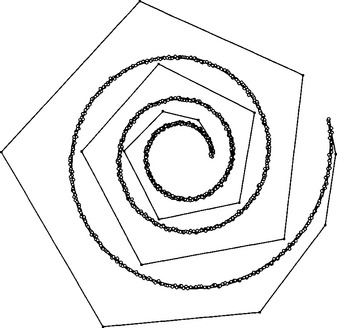
Figures 9.1 through 9.4 give some examples. In all four figures, 1,000 points were sampled from a spiral, and noise was added. The parameter values were assigned according to the centripetal parametrization; the knots were assigned uniformly. The best fit and shape is obtained, not surprisingly, by using a relatively high degree and many intervals; see Figure 9.4. The corresponding curvature plots are shown in Figure 23.1.

After the curve p(u) has been computed, we will find that many distance vectors pi – p(wi) are not perpendicular to ![]() (wi). This means that the point p(wi)on the curve is not the closest point to pi, and thus
(wi). This means that the point p(wi)on the curve is not the closest point to pi, and thus ![]() pi – p(wi)
pi – p(wi) ![]() does not measure the distance of pi to the curve. This indicates that we could have chosen a better data parameter value wi corresponding to pi. We may improve our estimate for wi by finding the closest point to pi on the computed curve and assigning its parameter value
does not measure the distance of pi to the curve. This indicates that we could have chosen a better data parameter value wi corresponding to pi. We may improve our estimate for wi by finding the closest point to pi on the computed curve and assigning its parameter value ![]() to pi; see Figure 9.5. We do this for all i and then recompute the least squares curve with the new
to pi; see Figure 9.5. We do this for all i and then recompute the least squares curve with the new ![]() . This process typically converges after three or four iterations.4 It was named parameter correction by J. Hoschek [337], [577].
. This process typically converges after three or four iterations.4 It was named parameter correction by J. Hoschek [337], [577].

Figure 9.5 Parameter correction: the connection of pi and p(wi) is typically not perpendicular to the tangent at p(wi). A better value for wi is found by projecting pi onto the tangent.


Figure 9.3 Least squares approximation: n = 3, K = 15, smoothing factor α = 0.05. Figure courtesy M. Jeffries.
The new parameter value ![]() is found using a Newton iteration. We project pi onto the tangent at p(wi), yielding a point qi. Then the ratio of the lengths
is found using a Newton iteration. We project pi onto the tangent at p(wi), yielding a point qi. Then the ratio of the lengths ![]() is a measure for the adjustment of wi. The actual Newton iteration step looks like this:
is a measure for the adjustment of wi. The actual Newton iteration step looks like this:
In this equation,![]() denotes the arc length of the segment that wi is in, that is, uk<wi ≤ uk+1. This length may safely (and cheaply) be overestimated by the length of the Bézier polygon of the kth segment.
denotes the arc length of the segment that wi is in, that is, uk<wi ≤ uk+1. This length may safely (and cheaply) be overestimated by the length of the Bézier polygon of the kth segment.
We finally note that (9.8) should not be used to compute the point on a curve closest to an arbitrary point pi. It works only if pi is close to the curve, and if a good estimate wi is known for the closest point on the curve.
9.3 Modifying B-Spline Curves
The use of B-spline curves is often described like this: pick a control point, move it, observe the shape of the resulting curve, and stop once a desired shape is obtained. It is more intuitive, however, to let a user pick a point on the curve, move it to a new position, and then compute a control polygon that will accommodate this change. We already did this for the case of Bézier curves in Section 7.10.
Having solved the Bézier case makes the corresponding B-spline problem a relatively easy task. Suppose we want to change a point x(û) on a B-spline curve. Because of the local control property of B-spline curves, this point is determined by n + 1 B-spline control points di. With some relabeling, we can write it as
We wish to find new control points di such that the new curve goes through a point y for parameter value Û. This is exactly the same problem as for the Bézier case if we want to change only d1,…, dn–1. If changing all vertices d0, …, dn is desired, the linear system has to be changed to
This is a linear system consisting of one equation for n + 1 unknowns and is solved as in Section 7.10. Figure 9.6 gives an example.

Figure 9.6 Modifying B-spline curves: a point on a cubic B-spline curve is moved and a new polygon is computed that passes through the new point.
It is possible to change not only a point on a curve. Since this results in an underdetermined system, more constraints such as more point changes or prescription of derivatives may be added. This was covered in detail by Bartels and Forsey [48].
9.4 C2 Cubic Spline Interpolation
This is the most popular of all spline algorithms. For this section, we will use the condensed form of the knot sequence, denoting each knot as τi. We will be dealing only with knot sequences that are simple (μi = 1) except for the end knots that are of multiplicity three: μ0= 3, μk = 3.
The problem statement is as follows:
Given: A set of data points p0,… ., pK and a knot sequence τ0, τk and a multiplicity vector 3, 1, 1, …, 1, 1, 3.
Find: A set of B-spline control points d0, …, dL with L = K + 2 such that the resulting C2 piecewise cubic curve x(u) satisfies
Consult Figure 9.7 for an example of the numbering scheme.

As it turns out, the preceding problem is ill posed: the number of unknowns is K + 3, whereas the number of given data points is K + 1. This is an underdetermined problem; two more conditions are needed in order to have a uniquely solvable problem. We will discuss several possibilities for this; to begin with, we consider clamped end conditions.
A clamped end condition corresponds to the prescription of two derivatives ![]() and
and ![]() . They are given by
. They are given by
The geometry of this interpolation problem is illustrated in Figure 9.7
Because of the triple end knots, we immediately have
this takes care of equations #0 and #K of (9.10). We will not use these in setting up our linear system.
The clamped end conditions yield
Thus, the first and last equations of our linear system become
with
Each of the remaining unknowns d2, …, dL–2 is related to the data points by one equation. Because of the local support property of cubic B-splines, it is of the form
Together, these are K – 1 equations for the K – 1 unknown control points. In matrix form, we have
Schematically, the case K = 5 looks like this:

The entries in this tridiagonal matrix are easily computed from the definitions of the cubic B-splines Ni3.
In the case of uniform knots ui = i, the interpolation conditions (9.11) take on a particularly simple form:
We conclude with a method for cubic spline interpolation that occasionally appears in the literature (e.g., in Yamaguchi [621]). It is possible to solve the interpolation problem without setting up a linear system! Just do the following: define d0, d1, dL–1, dL as before, and set di = pi–1 for all other control points. Then, for i = 2, …, L – 2, correct the location of di such that the curve passes through pi–1. Repeat until the solution is found.
This method will always converge and will not need many steps in order to do so. So why bother with linear systems? The reason is that tridiagonal systems are most effectively solved by a direct method, whereas the earlier iterative method amounts to solving the system via Gauss-Seidel iteration. So though geometrically appealing, the iterative method needs more computation time than the direct method.
9.5 More End Conditions
For cubic spline interpolation, the choice of end conditions is important for the shape of the interpolant near the endpoints—they do not matter much in the interior. We have seen a clamped end condition earlier. It works well in situations where the end derivatives are actually known. But in most applications, we do not have this knowledge. Still, two extra equations are needed in addition to the basic interpolation conditions (9.10).
We list several possibilities:
The natural end conditions are derived from the physical analogy of a wooden beam that is clamped at some positions; see Figure 9.22. Beyond the first and last clamps, such a beam assumes the shape of a straight line. A line is characterized by having a zero second derivative, and hence the end conditions
Figure 9.22 Spline interpolation: a plastic beam, the spline, is forced to pass through data points, marked by metal weights, the ducks.
are called natural end conditions.
The second derivative of a Bézier curve at b0 is given by b0 – 2b1 + b2. In terms of B-spline control vertices (using triple end knots), this becomes
where we set Δi = τi+1 – τi. We rearrange and obtain
A similar condition holds at the other endpoint. Unless required by a specific application, this end condition should be avoided since it forces the curve to behave linearly near the endpoints.
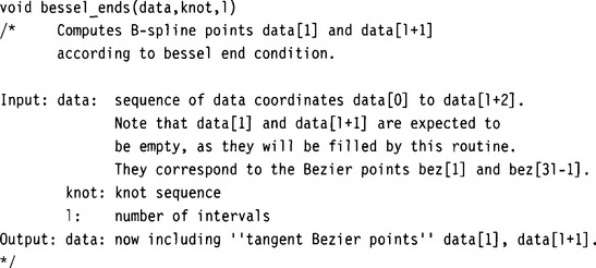
Typically another end condition, called Bessel end condition, yields better results. It works as follows: the first three data points and their parameter values determine an interpolating quadratic curve. Its first derivative at p0 is taken to be the one for the spline curve. If we set
and
then
This value for d1 is then used in the earlier clamped end condition. The control point dL–1 is obtained in complete analogy; it is then also used for a clamped end condition.
Other end conditions exist: requiring ![]() is called a quadratic end condition. If all data points and parameter values were read off from a quadratic curve, then this condition would ensure that the spline interpolant reproduces that quadratic. The same is true, of course, for the Bessel end conditions. If the first and second cubic segment are parts of one cubic, then their third derivatives at τ1 would agree. The corresponding end condition is called not-a-knot condition since the knot τ1 does not act as a breakpoint between two distinct cubic segments.
is called a quadratic end condition. If all data points and parameter values were read off from a quadratic curve, then this condition would ensure that the spline interpolant reproduces that quadratic. The same is true, of course, for the Bessel end conditions. If the first and second cubic segment are parts of one cubic, then their third derivatives at τ1 would agree. The corresponding end condition is called not-a-knot condition since the knot τ1 does not act as a breakpoint between two distinct cubic segments.
We finish this section with a few examples, courtesy T. Foley, using uniform parameter values in all examples.5 Figure 9.8 shows equally spaced data points read off from a circle of radius 1 and the cubic spline interpolant obtained with clamped end conditions, using the exact end derivatives of the circle. Figure 9.9 shows the curvature plot 6 of the spline curve. Ideally, the curvature should be constant, and the spline curvature is quite close to this ideal.

Figure 9.10 shows the same data, but now using Bessel end conditions. Near the endpoints, the curvature deviates from the ideal value, as shown in Figure 9.11.


Finally, Figure 9.12 shows the curve that is obtained using natural end conditions. The end curvatures are forced to be zero, causing considerable deviation from the ideal value, as shown in Figure 9.13. This end condition should be avoided unless the linear behavior near the ends is desired.


9.6 Finding a Knot Sequence
The spline interpolation problem is usually stated as “given data points pi and parameter values ui, … .” Of course, this is the mathematician’s way of describing a problem. In practice, parameter values are rarely given and therefore must be made up somehow. The easiest way to determine the ui is simply to set ui = i. This is called uniform or equidistant parametrization. This method is too simplistic to cope with most practical situations. The reason for the overall poor 7 performance of the uniform parametrization can be blamed on the fact that it “ignores” the geometry of the data points.
The following is a heuristic explanation of this fact. We can interpret the parameter u of the curve as time. As time passes from time u0 to time uL, the point x(u) traces the curve from point x(u0) to point x(uL). With uniform parametrization, x(u) spends the same amount of time between any two adjacent data points, irrespective of their relative distances. A good analogy is a car driving along the interpolating curve. We have to spend the same amount of time between any two data points. If the distance between two data points is large, we must move with a high speed. If the next two data points are close to each other, we will overshoot since we cannot abruptly change our speed—we are moving with continuous speed and acceleration, which are the physical counterparts of a C2 parametrization of a curve. It would clearly be more reasonable to adjust speed to the distribution of the data points.
One way of achieving this is to have the knot spacing proportional to the distances of the data points:
A knot sequence satisfying (9.15) is called chord length parametrization. Equation (9.15) does not uniquely define a knot sequence; rather, it defines a whole family of parametrizations that are related to each other by affine parameter transformations. In practice, the choices u0 = 0 and uL = 1 or u0 = 0 and uL = L are reasonable options.
Chord length usually produces better results than uniform knot spacing, although not in all cases. It has been proven (Epstein [186]) that chord length parametrization (in connection with natural end conditions) cannot produce curves with corners 8 at the data points, which gives it some theoretical advantage over the uniform choice.
Another parametrization has been named “centripetal” by E. Lee [378]. It is derived from the physical heuristics presented earlier. If we set

the resulting motion of a point on the curve will “smooth out” variations in the centripetal force acting on it.
Yet another parametrization was developed by G. Nielson and T. Foley [449]. It sets
where dj = ![]() Δ pi
Δ pi ![]() and
and
and Θi is the angle formed by Pi–1, pi, pi+1 Thus ![]() is the “adjusted” exterior angle formed by the vectors Δpi and Δpi+1. As the exterior angle
is the “adjusted” exterior angle formed by the vectors Δpi and Δpi+1. As the exterior angle ![]() increases, the interval Δi increases from the minimum of its chord length value up to a maximum of four times its chord length value. This method was created to cope with “wild” data sets.
increases, the interval Δi increases from the minimum of its chord length value up to a maximum of four times its chord length value. This method was created to cope with “wild” data sets.
We note one property that distinguishes the uniform parametrization from its competitors: it is the only one that is invariant under affine transformations of the data points. Chord length, centripetal, and the Foley methods all involve length measurements, and lengths are not preserved under affine maps. One solution to this dilemma is the introduction of a modified length measure, as described in Nielson [446].9
For more literature on parametrizations, see Cohen and O’Dell [122], Hartley and Judd [314], [315], McConalogue [421], and Foley [239].
Figures 9.14 to 9.2110 show the performance of the discussed parametrization methods for one sample data set. For each method, the interpolant is shown together with its curvature plot. For all methods, Bessel end conditions were chosen.

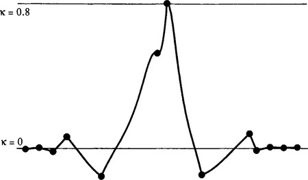


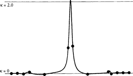

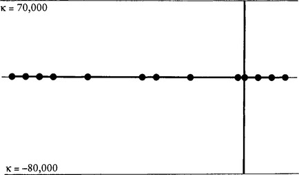
Although the figures are self-explanatory, some comments are in order. Note the very uneven spacing of the data points at the marked area of the curves. Of all methods, Foley’s copes best with that situation (although we add that many examples exist where the simpler centripetal method wins out). The uniform spline curve seems to have no problems there, if one just inspects the plot of the curve itself. However, the curvature plot reveals a cusp in that region! The huge curvature at the cusp causes a scaling in the curvature plot that annihilates all other information. Also note how the chord length parametrization yields the “roundest” curve, having the smallest curvature values, but exhibiting the most marked inflection points.
There is probably no “best” parametrization, since any method can be defeated by a suitably chosen data set. The following is a (personal) recommendation. You may improve the shape of the curve, at an increase of computation time, by the following hierarchy of methods: uniform, chord length, centripetal, Foley. The best compromise between cost and result is probably achieved by the centripetal method.
9.7 The Minimum Property
In the early days of design, say, ship design in the 1800s, the problem had to be handled of how to draw (manually) a smooth curve through a given set of points. One way to obtain a solution was the following: place metal weights (called ducks) at the data points, and then pass a thin, elastic wooden beam (called a spline) between the ducks. The resulting curve is always very smooth and usually aesthetically pleasing. The same principle is used today when an appropriate design program is not available or for manual verification of a computer result; see Figure 9.22.
The plastic or wooden beam assumes a position that minimizes its strain energy. The mathematical model of the beam is a curve s, and its strain energy E is given by
where κ denotes the curvature of the curve. The curvature of most curves involves integrals and square roots and is cumbersome to handle; therefore, one often approximates the preceding integral with a simpler one:
Note that ![]() is a vector; it is obtained by performing the integration on each component of s.
is a vector; it is obtained by performing the integration on each component of s.
Equation (9.18) is more directly motivated by the following example: when an airplane is scheduled to fly from A to B, it will have to fly over a number of intermediate “way points.” The amount of fuel used by an airplane is mostly affected by its acceleration, which is essentially equivalent to the second derivative of its trajectory. Thus if the plane follows a cubic spline curve passing through all the way points, it will be guaranteed to use the least amount of fuel!11
In a more general setting, we may word this as: among all C2 curves interpolating the given data points at the given parameter values and satisfying the same end conditions, the cubic spline yields the smallest value for each component of Ê. For a proof, let s(u) be the C2 cubic spline and let y(u) be another C2 interpolating curve. We can write y as
The preceding integrals are defined componentwise; we will show the minimum property for one component only. Let s(u) and y(u) be the first component of s and y, respectively. The “energy integral” ![]() of y’s first component becomes
of y’s first component becomes
We may integrate the middle term by parts

The first term vanishes because of the common end conditions. In the second term, ![]() is piecewise constant:
is piecewise constant:

All terms in the sum vanish because both s and y interpolate. Since
for continuous ![]()
we have proved the claimed minimum property.
The minimum property of splines has spurred substantial research activity. The replacement of the actual strain energy measure E by ![]() is motivated by the desire for mathematical simplicity. The curvature of a curve is given by
is motivated by the desire for mathematical simplicity. The curvature of a curve is given by
But we need ![]() in order for
in order for ![]() to be a good approximation to κ. This means, however, that the curve must be parametrized according to arc length; see (10.7). This assumption is not very realistic for cubic splines in a design environment; see Problems.
to be a good approximation to κ. This means, however, that the curve must be parametrized according to arc length; see (10.7). This assumption is not very realistic for cubic splines in a design environment; see Problems.
While the classical spline curve merely minimizes an approximation to (9.18), methods have been developed that produce interpolants that minimize the true energy (9.18), see [425], [99]. Moreton and Séquin have suggested to minimize the functional ![]() instead; see [431].
instead; see [431].
9.8 C1 Piecewise Cubic Interpolation
Spline curves come in the B-spline form, but they may also be described as piecewise Bézier curves. We now consider that approach, applied to piecewise cubic interpolation. First, we try to solve the following problem:
Given: Data points x0, …, xL and tangent directions 10, …,1L at those data points; see Figure 9.23.

Find: A C1 piecewise cubic polynomial that passes through the given data points and is tangent to the given tangent directions there.
It is important to note that we only have tangent directions, that is, we have no vectors with a prescribed length since our problem statement did not involve a knot sequence. We can assume without loss of generality that the tangent directions 1i have been normalized to be of unit length:
The easiest step in finding the desired piecewise cubic is the same as before: the junction Bézier points b3i are again given by b3i = xi, i = 0, …, L.
For each inner Bézier point, we have a one-parameter family of solutions: we only have to ensure that each triple b3i–1, b3i, b3i+1 is collinear on the tangent at b3i, and ordered by increasing subscript in the direction of 1i. We can then find a parametrization with respect to which the generated curve is C1 [see (5.30)].
In general, we must determine the inner Bézier points from
so that the problem boils down to finding reasonable values for αi and βi. Although any nonnegative value for these numbers is a formally valid solution, values for αi and βi that are too small cause the curve to have a corner at xi, whereas values that are too large can create loops. There is probably no optimal choice for αi and βi that holds up in every conceivable application—an optimal choice must depend on the desired application.
A “quick and easy” solution that has performed decently many times (but also failed sometimes) is simply to set
(The factor 0.4 is, of course, heuristic.)
The parametrization with respect to which this interpolant is C1 is the chord length parametrization. It is characterized by
A more sophisticated solution is the following: if we consider the planar curve in Figure 9.24, we see that it can be interpreted as a function, where the parameter t varies along the straight line through b3i and b3i+3. Then
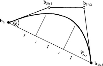
Figure 9.24 Inner Bézier points: this planar curve can be interpreted as a function in an oblique coordinate system with b3i, b3i+3 as the x-axis.
We are dealing with parametric curves, however, which are in general not planar and for which the angles Θ and Ψ could be close to 90 degrees, causing the preceding expressions to be undefined. But for curves with Θi, Ψi+1 smaller than, say, 60 degrees, these expressions could be used to find reasonable values for αi and βi:
Since cos 60° = 1/2, we can now make a case distinction:

and

This method has the advantage of having linear precision. It is C1 when the knot sequence satisfies Δi/Δi+1 = βi/αi+1.
Note that neither of these two methods is affinely invariant: the first method—(9.22)—does not preserve the ratios of the three points b3i–1, b3i, b3i+1 since the ratios ![]() Δxi–1
Δxi–1![]() :
: ![]() Δxi
Δxi![]() are not generally invariant under affine maps.12 The second method uses angles, which are not preserved under affine transformations. However, both methods are invariant under euclidean transformations. We now address a different version of piecewise cubic interpolation:
are not generally invariant under affine maps.12 The second method uses angles, which are not preserved under affine transformations. However, both methods are invariant under euclidean transformations. We now address a different version of piecewise cubic interpolation:
Given: Data points x0, …,xL together with corresponding parameter values u0, …, uL.
Find:A C1 piecewise cubic polynomial that passes through the given data points.
One solution to this problem is provided by C2 (and hence also C1) cubic splines, which are discussed in Section 9.4. Although those provide a global solution, a local one might be preferred for some applications where C2 smoothness is not crucial. We are then faced with the problem of estimating tangents from the given data points and parameter values.
The simplest method for tangent estimation is known under the name FMILL. It constructs the tangent direction li at xi to be parallel to the chord through xi–1 and xi+1:
Once the tangent direction vi has been found,13 the inner Bézier points are placed on it according to Figure 9.25:
This interpolant is also known as a Catmull–Rom spline.

This construction of the inner Bézier points does not work at x0 and xL. The next method, Bessel tangents, does not have that problem.
The idea behind Bessel tangents14 is as follows: to find the tangent vector mi at xi, pass the interpolating parabola qi(u) through xi–1, xi, xi+1 with corresponding parameter values ui–1, ui, ui+1 and let mi be the derivative of qi. We differentiate qi at ui:
Written in terms of the given data, this gives
where
The endpoints are treated in the same way: m0 = d/duq1(u0), mL = d/duqL–1(uL), which gives
Another interpolant that makes use of the parabolas qi is known as an Overhauser spline, after work by A. Overhauser [452] (see also [91] and [154]). The ith segment si of such a spline (defined over [ui, ui+1]) is defined by
In other words, each si is a linear blend between qi and qi+1. At the ends, one sets s0(u) = q0(u) and sL–1(u) = qL–1(u).
On closer inspection, it turns out that the last two interpolants are not different at all: they both yield the same C1 piecewise cubic interpolant (see Problems). A similar way of determining tangent vectors was developed by McConalogue [421], [422].
Finally, we mention a method created by H. Akima [3]. It sets
where
and
This interpolant appears fairly involved. It generates very good results, however, in situations where curves are needed that oscillate only minimally.
9.9 Implementation
The following routines produce the cubic B-spline polygon of an interpolating C2 cubic spline curve. First, we set up the tridiagonal linear system:

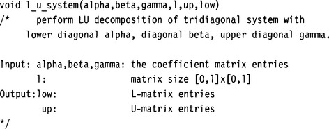
The next routine performs the LU decomposition of the matrix from the previous routine. (Note that we do not generate a full matrix but rather three linear arrays!)
Finally, the routine that solves the system for the B-spline coefficients di:

In case Bessel ends are desired instead of clamped ends, this is the code:
The centripetal parametrization is achieved by the following routine:

A calling sequence that uses the preceding programs might look like this:
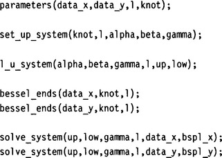
Here, we solved the 2D interpolation problem with given data points in data– x, data–y, a knot sequence knot, and the resulting B-spline polygon in bspl–x, bspl–y. This calling sequence is realized in the routine c2–spline.c.
9.10 Problems
1. For the case of closed curves, C1 quadratic spline interpolation with uniform knots does not always have a solution. Why?15
*2. Show that interpolating splines reproduce cubic polynomial curves—that they have cubic precision. This means that if all data points pi are read off from a cubic, pi = c(ui), and the end tangent vectors are read off from the cubic, then the interpolating spline equals the original cubic.
3. Show that Akima’s interpolant always passes a straight line segment through three subsequent points if they happen to lie on a straight line.
*4. Show that Overhauser splines are piecewise cubics with Bessel tangents at the junction points.
*5. One can generalize the quintic Hermite interpolants from Section 7.6 to piecewise quintic Hermite interpolants. These curves need first and second derivatives as input positions. Devise ways to generate second derivative information from data points and parameter values.
P1. Using piecewise cubic C1 interpolation, approximate the semicircle with radius 1 to within a tolerance of ∈ = 0.001. Use as few cubic segments as possible. Literature: [172], [260].
P2. Program the following: instead of prescribing end conditions for interpolating C2 splines at both ends, prescribe first and second derivatives at ![]() . The interpolant can then be built segment by segment. Discuss the numerical aspects of this method (they will not be wonderful).
. The interpolant can then be built segment by segment. Discuss the numerical aspects of this method (they will not be wonderful).
1Many explicit wing section equations are given by the so-called NACA profiles.
2We are thus assuming that the data points are numbered in a meaningful order. The problem changes completely if this assumption is not valid, see [382].
3Note that wi does not have to be one of the knots!
4In theory, more iterations should produce better fits. In practice, however, the fit often deteriorates after more than four iterations.
5Owing to the symmetry inherent in the data points, all parametrizations discussed later yield the same knot spacing. All circle plots are scaled down in the y-direction.
6The graph of curvature versus arc length; see also Chapter 23.
7There are cases in which uniform parametrization fares better than other methods. An interesting example is in Foley [239], p. 86.
8A corner is a point on a curve where the tangent (not necessarily the tangent vector!) changes in a discontinuous way. The special case of a change in 180 degrees is called a cusp; it may occur even using the chord length parametrization.
9The Foley parametrization was in fact first formulated in terms of that modified length measure.
10Kindly provided by T. Foley.
11I am grateful to P. Crouch for bringing the airplane analogy to my attention.
12Recall that only the ratio of three collinear points is preserved under affine maps!
13Note that here we do not have ![]() vi
vi![]() = 1!
= 1!
14They are also attributed to Ackland [2].
15T. DeRose pointed this out to me.