Surfaces with Arbitrary Topology
The surfaces that we have met so far are best suited for shapes that are the image of some part of the plane—of a rectangle in the case of B-spline or Bézier surfaces, of a triangulated region in the case of composite Bézier triangles. This limits the topology of these surfaces; for example, it is not possible to construct even a sphere without introducing degenerate patches while using a C1 map of a part of the plane. Even shapes that have the topology of a planar region may be too complex to model with one tensor product surface; just imagine modeling a glove that way. The complexity issue may be tackled using the approach of hierarchical B-spline surfaces as proposed by Forsey and Bartels [245]. But even with this method, arbitrary topology is not achievable.
In this chapter, we will investigate methods that are suited for the construction of shapes of arbitrary complexity and/or topology. We can present only a brief selection of methods; more literature on the topic: [177], [596], [595], [594], [289], [290], [293], [321], [431], [627], [398], [561]. The first in-depth study of recursive subdivision processes goes back to U. Reif [503]. The basic concepts of surface topology are nicely explained in [323].
21.1 Recursive Subdivision Curves
We already encountered Chaikin’s algorithm in Section 8.4. Starting with a polygon, it produces a sequence of refined polygons that ultimately converge to the uniform quadratic B-spline curve defined by the initial polygon.
This principle may be applied to higher-degree uniform splines; we discuss the cubic case here. If we double a uniform knot sequence by inserting the midpoint of every knot, new control points ![]() are generated from the existing ones by setting
are generated from the existing ones by setting

See Figure 21.1 for an illustration. We may analyze the resulting curve by exploiting the fact that we are dealing with a cubic B-spline curve. However, that analysis may also be carried out without this knowledge. Let us investigate the limit of the sequence ![]() . We may write the recursion in matrix form as
. We may write the recursion in matrix form as
and abbreviate it as
The matrix A has eigenvalues ![]() and may be diagonalized1 as
and may be diagonalized1 as
where

The matrix E contains A’s eigenvectors, and the diagonal matrix Λ contains A’s eigenvalues.
For the next iteration, we have
Using our diagonalization for A, we get
and further
Taking the limit r → ∞ yields
Since
this becomes
implying that all three points dk–1, dk, dk+1 converge to the same point (dk–1+ 4dk + dk+1)/6. This result is no surprise since we know we are dealing with B-spline curves. It does illustrate, however, a general principle that is ubiquitous in all subdivision theory, namely, that convergence analysis is normally carried out via an eigenvalue analysis.
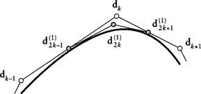
Subdivision may also be used to generate interpolating curves. The basic four-point principle was developed by Dyn, Levin, and Gregory [178], [176]. Let a sequence of points pi be given; then successively construct new sequences by setting

For an illustration, see Figure 21.2. The point ![]() is the result of applying cubic Lagrange interpolation at uniform knots, see [519].
is the result of applying cubic Lagrange interpolation at uniform knots, see [519].
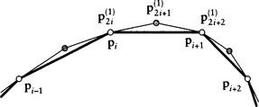
At each level of the subdivision process, the points of the previous step are retained; this causes the scheme to interpolate to the initial set of points. The limit curve is C1, but fails to be C2.
21.2 Doo–Sabin Surfaces
The fundamental idea of this kind of surface goes back to Chaikin’s algorithm; see Section 8.4. There, we started with a polygon, iteratively applied a refinement procedure to it, and observed that in the limit we ended up with a smooth curve. M. Sabin and D. Doo asked if this principle could be carried over to surfaces: start with a polyhedron, iteratively apply a refinement procedure to it, and see if a smooth surface would result.
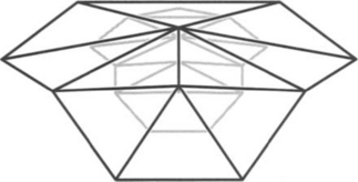
They then came up with the following algorithm, illustrated in Fig. 21.3 and documented in [174]: input: an arbitrary closed polyhedron with vertices pi. These vertices form (straight) edges and (not necessarily planar) faces, thus defining the topology of the polyhedron. The refinement step now becomes:

Step 2 needs some more explanation. The new polyhedron will have faces that are constructed according to three different rules:
2a. The F-faces are found by cyclically connecting the ![]() of each original face.
of each original face.
2b. The E-faces are found by considering any two original faces sharing a common edge: there are exactly four midpoints on the lines connecting each face centroid with the edge endpoints. These four points produce a four-sided face.
2c. The V-faces are formed by considering all E-faces around an original vertex. They surround a face that is “centered” on that vertex.
As we keep repeating the algorithm, it produces mostly four-sided faces. The only non-four-sided faces are V-faces generated by those initial vertices whose valency2 is not four, or F-faces whose initial faces are not four sided. These faces give rise to limit points whose valency is not four, so-called extraordinary vertices. In fact, it is not hard to see that after the first step the valency of every new vertex is four. In this manner, large regions of the new polyhedra are covered with nets that have a tensor product structure. Doo–Sabin surfaces are thus “mostly” biquadratic B-splines. See Figure 21.4 for an example.
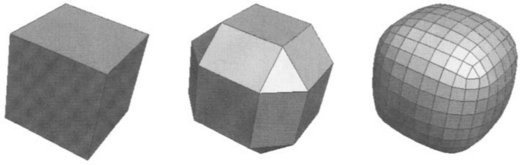
Figure 21.4 The Doo–Sabin algorithm: an example. Left, the original mesh (a cube). Middle, after one iteration. Right, after three iterations. Figure courtesy A. Nasri.
Let us briefly analyze the structure of the Doo–Sabin algorithm. New face points ![]() are created from previous ones in a linear fashion that lends itself to a matrix formulation. Let us consider a five-sided face such as the center face in Figure 21.3. We obtain
are created from previous ones in a linear fashion that lends itself to a matrix formulation. Let us consider a five-sided face such as the center face in Figure 21.3. We obtain

We may write this as
which becomes
after r applications of the algorithm. In the general case, we have the same structure but have to replace A5 by a matrix An for faces with n edges.
As r increases, the behavior of the subdivision process depends crucially on the eigenvalues of An since we may write ![]() as
as
following the approach of Section 21.1. Since all rows of An sum to unity, one eigenvalue is λ1 = 1. The remaining ones are all real since A is symmetric and are all between 0 and 1 since each V(k) is contained in the convex hull of V(k–1). An exact analysis of this process is fairly involved and is omitted here. It reveals, however, that Doo–Sabin surfaces are G1 everywhere. For more details, see [174] or [18], [19], [503]. The matrices An are circulant, and their eigenstructure has been studied in detail by P. Davis [134]. A matrix is circulant if each row may be obtained from the previous row by a “right shift.”
Figure 21.4 gives an example of several steps of the algorithm.
As a rather trivial observation, Doo–Sabin surfaces have the convex hull and local control properties, and their construction is affinely invariant. But they also do not need an underlying parametrization, which makes them more geometric than tensor product B-spline surfaces. A drawback of this nice feature is the problem of point evaluation: though we can evaluate as many points as close to the surface as we like, computation of just one point is not trivial.
One set of points on the surface is easy to identify: at every level of subdivision, the centroid of any face will be on the final surface. For a proof, we observe that any face will produce a sequence of F-faces converging to its centroid. In the limit, the centroid is thus on the surface.
21.3 Catmull–Clark Subdivision
The same issue of Computer-Aided Design that included the Doo–Sabin algorithm also contained a competing method, invented by E. Catmull and J. Clark; see [103]. Whereas Doo–Sabin surfaces are a generalization of biquadratic B-splines to arbitrary topology, Catmull–Clark surfaces generalize bicubic B-spline surfaces to arbitrary topology.
We start with a polygonal mesh ![]() consisting of vertices
consisting of vertices ![]() . We iteratively refine the mesh, resulting in finer and finer meshes
. We iteratively refine the mesh, resulting in finer and finer meshes ![]() consisting of vertices
consisting of vertices ![]() . Each refinement step can be described by explaining what happens locally for the points adjacent to a vertex vi:
. Each refinement step can be described by explaining what happens locally for the points adjacent to a vertex vi:
1. Form face points ![]() : for each face in the mesh, find the centroid of its vertices.
: for each face in the mesh, find the centroid of its vertices.
2. Form edge points ![]() : for each edge in the mesh, average the edge’s endpoints and the two face points on either side of the edge.
: for each edge in the mesh, average the edge’s endpoints and the two face points on either side of the edge.
3. Form a new vertex point vi+1: assuming there are n faces around vi, it is computed as follows:
4. Form new faces. Each new face consists of a loop of the form
where the two fi+1’s refer to the same face point.
Note that all faces after the first level will be four sided. The basic principle is shown in Figure 21.5. Figure 21.6 gives an example.
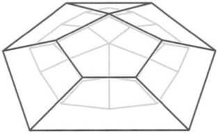
Figure 21.5 The Catmull–Clark algorithm: the original control net (black) and one level of subdivision (gray).

Figure 21.6 The Catmull–Clark algorithm: an example. Left, the original mesh (a cube). Middle, after one iteration. Right, after three iterations. Figure courtesy A. Nasri.
For the example of a vertex with valency n = 4, the relationship between new and old vertices may be expressed as a matrix equation:

For valencies other than four, similar matrix equations hold; see [308]. Those vertices converge to extraordinary vertices.
We may abbreviate (21.3) as
An equivalent form of (21.9) is given by
We note that the matrix A must be stochastic; that is, the elements of each row must sum to one. This is a consequence of the fact that (21.8) represents a barycentric combination. We further note that our mesh refinement consists of taking convex combinations at each level: this implies that all meshes ![]() lie in the convex hull of
lie in the convex hull of ![]()
It follows that A has the dominant eigenvalue 1; the magnitudes of all other (possibly complex) eigenvalues are bounded by 1.
A careful eigenvalue analysis (see Ball and Storry [18]) can now be used to show that
While Catmull–Clark surfaces are generalizations of uniform bicubic spline surfaces, a generalization of the nonuniform case also exists; it is described in [561].
21.4 Midpoint Subdivision
This algorithm is simpler than either Catmull–Clark or Doo–Sabin and goes back to Peters and Reif [469] who call it “the simplest scheme.”
1. Form edge points e: for each edge in the mesh, compute its midpoint.
2. Form faces of new level. There are two types: faces inscribed to the existing ones and faces whose vertices are the edge midpoints around old vertices. See Figure 21.7 for an illustration. In order to discuss convergence of the scheme, let pl …, pn be the vertices of a face. This face generates vertices ![]() as edge midpoints
as edge midpoints
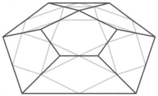
Figure 21.7 Midpoint subdivision: the original control net (black) and one level of subdivision (gray).
We write this as
Matrices of the form (21.12) are called circulant.
After k iterations, this becomes
The matrix M may be decomposed into a product
where E is the matrix containing M’s eigenvectors and Λ is the diagonal matrix containing M’s eigenvalues. We then have, following the reasoning in Section 21.1,
The analysis of the limit process is thus closely related to the eigenstructure of M. A result from Davis [134] asserts that for any initial polygon P, we obtain regular planar polygons in the limit. These will be the tangent planes to our surface, which therefore is G1.
21.5 Loop Subdivision
A triangle-based subdivision scheme was discussed by C. Loop [397]. Its input is a triangular mesh as discussed in Section 21.9. It then successively refines this mesh, resulting in a smooth limit surface.
Loop subdivision proceeds as follows.
1. Form edge points ![]() : assuming that
: assuming that ![]() and
and ![]() are the endpoints of an edge in the mesh and that
are the endpoints of an edge in the mesh and that ![]() and
and ![]() are the remaining vertices of the two triangles sharing the edge, set
are the remaining vertices of the two triangles sharing the edge, set
This process is easily visualized using a mask, shown in Figure 21.8. The coefficients shown are then multiplied by a factor of 1/8 in order to produce barycentric combinations.
2. For each vertex vi in the mesh, form a new vertex point vi+1. Assuming vi has n neighbors ![]() it is computed as follows:
it is computed as follows:
for n > 3 and ![]() if n = 3.
if n = 3.
3. Form new triangles. Figure 21.9 illustrates.
Now consider the mesh that is obtained after some number k of iterations. Select any vertex v of it. This vertex will converge to a point v∞ on the limit surface. Using an eigenvalue analysis as mentioned, we can show (see [584]) that this limit point is given by
where the vj are the neighbors of v in the mesh obtained after k iterations. For the special case k = 0, (21.15) gives the limit points corresponding to the original mesh vertices.
If all vertices in the mesh have valency six, then the resulting limit surface will be a collection of quartic Bézier triangles that form a C2 surface over an equilateral triangulation of a simply connected region of a (domain) plane. We note that closed surfaces cannot be formed using only points with valency six. Vertices with different valencies converge to extraordinary vertices, where the surface is only G1.
21.6  Subdivision
This scheme was developed by L. Kobbelt [362] and was also considered by Sabin [517]. We start with a triangular mesh and then subdivide each triangle into three triangles by splitting it at its centroid. Next, all edges of the initial mesh are flipped—instead of joining the initial vertices, they now join adjacent centroids. Finally, each initial vertex p (having valency n) is replaced by a barycentric combination of its neighbors:
where the neighbors of p are averaged to obtain c. The value for αn is set at
An example of one step of the ![]() scheme is shown in Figure 21.10.
scheme is shown in Figure 21.10.
Each subdivision step rotates the directional structure of the triangular mesh; after two applications, the initial orientation is reestablished. Each original triangle has then given rise to nine new triangles. Following a rigorous study of the eigenstructure of the ![]() operator, we can show that the resulting limit surface is G2 except at extraordinary points, where it still is G1.
operator, we can show that the resulting limit surface is G2 except at extraordinary points, where it still is G1.
21.7 Interpolating Subdivision Surfaces
When dealing with B-splines, we could start from a control polygon and design a curve, or we could start with data points and find an interpolating curve. We can also use recursive subdivision surfaces for interpolation. The idea goes back to Nasri [440] and to M. Lounsbery, S. Mann, and T. DeRose [402]. The latter reference constructs interpolating Catmull–Clark surfaces, whereas Nasri constructs interpolating Doo–Sabin surfaces—we will start with them.
Given is a polyhedron with vertices pi, and we wish to find another polyhedron with vertices vi such that the resulting Doo–Sabin surfaces pass through the pi. Each of the (unknown) vi will generate a V-face with vertices qi,k; k= 1, …, ni, where ni is the valency of vi. We know that the centroids of these V-faces are on the surface, and we simply require them to be the given data points:
Note that the given points are not on the faces of the desired polyhedron, but rather on the V-faces obtained from it after one level of subdivision; see Figure 21.11 for an illustration.
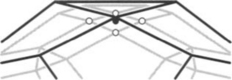
Figure 21.11 Interpolating Doo–Sabin surfaces: given points pi: solid. Intermediate points qi,k: hollow. Desired vertices vi: vertices of black mesh.
Since the relationship between the qi,k and the unknowns vi is known, we have a set of linear equations relating the given pi to the unknown vi. For closed polyhedra, the number of equations equals the number of unknowns, leading to a sparse linear system.
This method lends itself to a hybrid usage: some control mesh vertices vi may be given as with freeform design, whereas others are replaced by interpolation points pi Each of the interpolation points gives rise to one linear equation, and the resulting system is easily solved. See Figure 21.12 for an example.
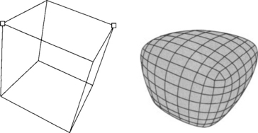
Figure 21.12 Interpolating Doo–Sabin surfaces: two vertices of the initial control net are marked as interpolation points. Resulting surface: right. (Courtesy A. Nasri.)
For open polyhedra, the situation is more complicated; it is dealt with by Nasri [439], [440], [441].
Catmull–Clark subdivision surfaces may also be employed to generate surfaces passing through a prescribed set of data points. We can use (21.11) to generate a control mesh that interpolates to a set of known data points v∞. All (21.11) form a linear system for the unknowns v1. This is a sparse system and thus quickly solved even if there are many (> 1000) data points.
It is mentioned in [308] that simply solving the least squares equations for the control points will result in “wiggly” surfaces. Adding shape equations as in Section 15.6 will overcome this problem.
In an similar fashion, (21.15) may be used to find a set of vertices vi that will generate a Loop surface through the data points pi. All these equations form a sparse linear system for the vi. It may be solved using a sparse solver or by an iterative method.
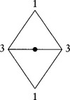
A more direct way to interpolation, that is, without the need to “invert” existing methods, is given by the butterfly scheme, due to Dyn, Gregory, and Levin [176]. Its structure is identical to Loop subdivision, but different weights are applied. At a given level in the refinement process, the vertex points are kept, and only new edge points are generated. Each new edge point is generated from the surrounding vertex points by a mask as shown in Figure 21.13. The (solid) edge point is obtained as a barycentric combination of nearby points; the coefficients in that combination are indicated in the figure. They have to be multiplied by a factor of 1/16.

Just as in the four-point curve interpolation scheme of Section 21.1, interpolation is assured since vertex points are kept.
21.8 Surface Splines
As we iterate through the Doo–Sabin algorithm, more and more of the surface is covered by biquadratic patches, just leaving the extraordinary regions. After two iterations, these are already nicely separated—they correspond to s-sided regions. J. Peters had the idea of deviating from the Doo–Sabin procedure after two steps and to fill in these s-sided regions with a collection of bicubics, such that the overall surface is G1; see [467] and also [466] or [463].3 It is not equivalent to the Doo–Sabin surface, but it has the advantage of being a collection of standard patches without singularities.
The situation after two (or more) steps of the Doo–Sabin algorithm is shown in Figure 21.14. We have so far created the points marked by squares. The solid squares mark control points surrounding an s-sided region, whereas the open ones are control points of the network of biquadratic patches. We are going to cover the s-sided region by a collection of s bicubic patches, all having a center point c in common. This center point is simply the average of all solid control points surrounding the s—sided region, only partially shown in Figure 21.14.
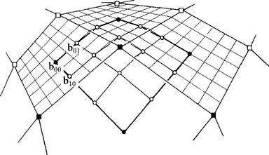
Figure 21.14 Surface splines: the control points determining the Bézier points bij of one bicubic patch.
Next, we have to degree elevate each quadratic boundary curve of the s-sided region and to subdivide it at its (parametric) midpoint. This gives two boundary curves of each bicubic patch.
The “outer” two layers of each bicubic patch lie on bilinear patches as shown in Figure 21.14. Their computation4 is illustrated for the four top left points in that figure:

The remaining eight Bézier points along the outer patch boundary are found analogously.
The three remaining Bézier points b22, b23, b32 are determined as follows:

where the superscript (i) refers to the ith bicubic patch of the patch collection covering the s-sided region. Now all angles ∠(b33, b32, b23) are equal. The points ![]() must be determined such that G1 continuity is ensured around b33. Setting c = cos(2π/s) and
must be determined such that G1 continuity is ensured around b33. Setting c = cos(2π/s) and ![]() , they are
, they are
A surface spline is shown in Figure 21.15.
Surface splines may also be used to interpolate to a mesh of data points in the same way as Doo–Sabin surfaces did: after two steps of the Doo–Sabin algorithm, move those control points that surround given data points such that their average equals that data point. Then proceed as before, and interpolation is ensured.
21.9 Triangular Meshes
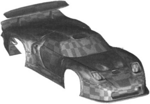
We encountered triangular meshes in Section 3.7—there, we were dealing with 2D meshes. Keeping the same data structure, we may generalize 2D triangulations to 3D triangle meshes: these are surfaces consisting of a collection of triangles; see Figure 21.16. The vertices pi of the triangles are now 3D points. Triangle meshes are piecewise linear and thus are not smooth—although this defect may be overcome by using very many triangles. One example is provided by the “Digital Michelangelo” project, carried out by M. Levoy. The aim of the project is to digitally record sculptures by Renaissance artist Michelangelo. Each sculpture was digitized using a laser digitizer; the resulting “point cloud” was then triangulated. For some sculptures, around two billion triangles were needed; see [386].

Figure 21.16 Triangular meshes: an example of a triangulated turbine. (Courtesy 3D Compression Technologies.)
Boundary edges are edges in the mesh that belong to one triangle only; all other edges, being part of two triangles, are called interior edges. A vertex is called boundary vertex if it is on a boundary edge; otherwise, it is called an interior vertex. The solid vertex in Figure 21.17 is an interior vertex.
A significant difference between 2D and 3D triangulations is their topology. Every 2D triangulation must have boundary vertices, but 3D triangulations do not have to have any. Consider the example of a tetrahedron, the simplest 3D triangle mesh. It has four vertices and four triangles, all of them interior vertices. Triangular meshes without boundaries are called closed; those that do have boundaries are called open.
Two additional examples of closed meshes are a triangulated sphere and a triangulated torus. A major difference between these is their genus, a number describing the topology of a mesh. The genus of a closed mesh is the number of holes it has. Thus a sphere has genus zero, a torus has genus one, a double torus has genus two, and so forth. If we denote the number of faces, edges, and vertices by f, e, v, respectively, then the following equation may be used to define the genus G:
This is known as the Euler-Poincaré formula and is valid even for meshes with polygonal faces, not just triangular ones. For example, a cube consisting of six square faces, twelve edges, and eight vertices, has genus 0. If we split each square into two triangles, we have (f, e, v) = (12, 18, 8), again resulting in genus zero. For more details, see Hoffmann [327].
21.10 Decimation
In many cases, triangulations are far too dense for an efficient representation of an object. What is called for then is a reduction in size, also known as decimation.5The goal is to remove as many points as possible, while still staying close to the initial triangulation.
A decimation algorithm will thus perform a check on every point and determine if it can be removed. If so, the point (and sometimes its neighbors) are removed and the resulting gap will be retriangulated. The process continues until no more data can be removed.
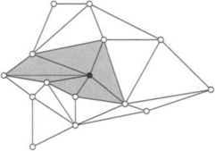
An important ingredient in many mesh algorithms is a test for determining if a mesh is flat in the vicinity of a vertex p. For the following, we will need the concept of the star ![]() of a vertex pi: this is the set of all triangles having pi as a vertex; see Figure 21.17. Thus the star of a point is itself a triangle mesh.
of a vertex pi: this is the set of all triangles having pi as a vertex; see Figure 21.17. Thus the star of a point is itself a triangle mesh.
In order to check if the mesh is flat around p, we compute the angles between all pairs of neighboring triangles in p![]() . If the largest of these angles is less than a given tolerance, then we label p as flat. The tolerance is naturally application dependent, but 0.1 to 1 degrees should work well. This flatness test is independent of scalings of the mesh since angles are not affected by scales.
. If the largest of these angles is less than a given tolerance, then we label p as flat. The tolerance is naturally application dependent, but 0.1 to 1 degrees should work well. This flatness test is independent of scalings of the mesh since angles are not affected by scales.
A different flatness criterion is due to M. Garland and P. Heckbert [254]. It locally constructs a quadric that approximates the neighborhood of a vertex. If the vertex is within a prescribed tolerance to this quadric, then it is labeled removable. This test is scale dependent: if the mesh is scaled, then the tolerance has to be scaled as well.
We now discuss a decimation method that is due to M. Lounsbery [400], [401]. It checks if an edge in a triangulation can be safely removed. If so, the edge is replaced by a point on it, thereby replacing two points by one. Retriangulation is fairly trivial: Figure 21.18 gives an example. A simple choice for the edge replacement point is the midpoint of the edge; more elaborate methods place it such that the shape of the resulting triangles is optimized.

Figure 21.18 Edge collapse: an edge is marked for collapsing, left. It is then collapsed into a single point, right.
When can an edge be removed? We simply perform a flatness test on the two edge vertices. If both meet the criterion, then the edge may be removed. Before that happens, it is advisable to check if the new triangles are within a specified tolerance to the old ones. An example of a decimated mesh is shown in Figure 21.19. This decimation method lends itself well to a multiresolution analysis of a triangle mesh. If we keep track of each collapsed edge, we create a hierarchy of triangle meshes. Each vertex in that hierarchy “knows” if it was generated by an edge collapse. The inverse process—recreating an edge from a vertex—is known as vertex split. Thus a heavily decimated mesh may be refined by successively adding in more edges using vertex splits. This successive refinement lends itself to streaming data transfer. More literature on multiresolution methods: [184], [183], [331], [330], [355].
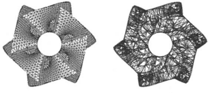
Figure 21.19 Decimation: the data set of Figure 21.16 (left), and after decimation (right). (Courtesy 3D Compression Technologies.)
A different decimation strategy is to remove a vertex, not an edge; this is due to Schroeder, Zarge, and Lorensen [545]. If a vertex is labeled removable, it is deleted and its star is retriangulated, see Figure 21.20.

Figure 21.20 Vertex removal: a vertex is labeled removable (left), and its star is retriangulated (right).
For more literature on mesh decimation, see [116], [404], [544].
21.11 Problems
1. Consider the following subdivision method: starting with a closed polygonal mesh, recursively subdivide by alternating between the Doo–Sabin and Catmull–Clark schemes. What can you say about the number of extraordinary vertices?
2. The Euler-Poincaré formula (21.16) always produces a genus that is an integer. Why?
3. Take a cube with square faces and place three square holes through it, each hole connecting opposite faces. What is the genus of the resulting object?
4. Sketch the effect of two levels of the ![]() scheme.
scheme.
*5. The Doo–Sabin recursion generates a sequence of F-faces for every face, in the limit converging to the centroid of the considered face. Show that the limiting F-faces are planar.
*6. Each of the triangles in p![]() forms an angle at p. Call the sum of all these angles ΣP. If ΣP = 360, then all triangles are in one plane. Thus the quantity 360 – |ΣP| measures the nonplanarity of p
forms an angle at p. Call the sum of all these angles ΣP. If ΣP = 360, then all triangles are in one plane. Thus the quantity 360 – |ΣP| measures the nonplanarity of p![]() —yet it is not a good flatness indicator. Why?
—yet it is not a good flatness indicator. Why?
P1. Write a program to find an interpolating Doo–Sabin surface to the eight vertices of a cube.
1The process of diagonalization is a standard linear algebra procedure.
2The valency of a vertex is the number of edges emanating from it.
3For a similar treatment of Catmull-Clark meshes, see [468].
4We give a slightly simplified version of Peters’s original development [467] here.
5The origin of the word can be traced to Roman times. When a legion fled during battle, it was punished by having every tenth soldier killed (decimated).