24.1 Bézier Curves or B-Spline Curves?

Taken at face value, this is a meaningless question: Bézier curves are a special case of B-spline curves. Any system that contains B-splines in their full generality, allowing for multiple knots, is capable of representing a Bézier curve or, for that matter, a piecewise Bézier curve.

In fact, several systems use both concepts simultaneously. A curve may be stored as an array holding B-spline control vertices, knots, and knot multiplicities. For evaluation purposes, the curve may then be converted to the piecewise Bézier form.

24.2 Spline Curves or B-Spline Curves?

This question is often asked, yet it does not make much sense. B-splines form a basis for all splines, so any spline curve can be written as a B-spline curve. What is often meant is the following: if we want to design a curve, should we pass an interpolating spline curve through data points, or should we design a curve by interactively manipulating a B-spline polygon? Now the question has become one concerning curve generation methods rather than curve representation methods.

A flexible system should have both: interpolation and interactive manipulation. The interpolation process may of course be formulated in terms of B-splines. Since many designers do not favor interactive manipulation of control polygons, we should allow them to generate curves using interpolation. Subsequent curve modification may also take place without display of a control polygon: for instance, the designer might move one (interpolation) point to a new position. The system could then compute the B-spline polygon modification that would produce exactly that effect. So a user might actually work with a B-spline package, but a system that is adapted to his or her needs might hide that fact. See Section 9.3 for details.

We finally note that every C² B-spline curve may be generated as an interpolating spline curve: read off junction points, end tangent vectors, and knot sequence from the B-spline curve. Feed these data into a C² cubic spline interpolator, and the original curve will be regenerated.

24.3 The Monomial or the Bézier Form?

We have made the point in this book that the monomial form¹ is less geometric than the Bézier form for a polynomial curve. A software developer, however, might not care much about the beauty of geometric ideas—in the workplace, the main priority is performance. Since the fundamental work by Farouki and Rajan [224], [225], [220], one important performance issue has been resolved: the Bézier form is numerically more stable than the monomial form. Farouki and Rajan observed that numerical inaccuracies, unavoidable with the use of finite precision computers, affect curves in the monomial form significantly more than those in Bézier form. More precisely, they show that the condition number of simple roots of a polynomial² is smaller in the Bernstein basis than in the monomial basis. If one decides to use the Bézier form for stability reasons, then it is essential that no conversions be made to other representations; these will destroy the accuracy gained by the use of the Bézier form. For example, it is not advisable from a stability viewpoint to store data in the monomial form and to convert to Bézier form to perform certain operations. More details are given in Daniel and Daubisse [132].

Figure 24.1 shows a numerical example, carried out using the routine bez_–to_– pow with single precision arithmetic. A degree 18 Bézier curve (top) was converted to the monomial form. Then, the coefficients of the Bézier and of the monomial form were perturbed by a random error, less than 0.001 in each coordinate. (The x-values of the control polygon extend from 0 to 20.) The Bézier curve shows no visual sign of perturbation, whereas the monomial form is not very reliable near t = 1. The experiment was then repeated for a degree 20 curve (bottom) with even more disastrous results. Although degrees like 18 or 20 look high, we should not forget that such degrees already appear in harmless-looking tensor product surfaces: for example, the diagonal u = v of a patch with n = m = 9 is of degree 18!

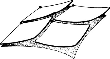
As a consequence of its numerical instability, the monomial form is not very reliable for the representation of curves or surfaces. For the case of surfaces, Figure 24.2 gives an illustration (in somewhat exaggerated form). Since the monomial form is essentially a Taylor expansion around the local coordinate (0.0) of each patch, it is quite close to the intended surface there. Farther away from (0,0), however, roundoff takes its toll. The point (1,1) is computed and therefore missed. For an adjacent patch, the actual point is stored as a patch corner, thus giving rise to the discontinuities shown in Figure 24.2. The significance of this phenomenon increases dramatically when curves or surfaces of high degrees are used.

Let’s not forget to mention the main attraction of the monomial form: speed. Horner’s method is faster than the de Casteljau algorithm; it is also faster than the routine hornbez. There is a tradeoff therefore between stability and speed. (Given modern hardware, things are not quite that clear-cut, however: T. DeRose and T. Holman [166] have developed a multiprocessor architecture that hardwires the de Casteljau algorithm into a network of processors and now outperforms Horner’s method.)

24.4 The B-Spline or the Hermite Form?

Cubic B-spline curves are numerically more stable than curves in the piecewise cubic Hermite form. This comes as no surprise, since some of the Hermite basis functions are negative, giving rise to numerically unstable nonconvex combinations. However, there is an argument in favor of the piecewise Hermite form: it stores interpolation points explicitly. In the B-spline form, they must be computed. Even if this computation is stable, it may produce roundoff.

A significant argument against the use of the Hermite form points to its lack of invariance under affine parameter transformations. Everyone who has programmed the Hermite form has probably experienced the trauma resulting from miscalculated tangent lengths. A programmer should not be burdened with the subtleties of the interplay between tangent lengths and parameter interval lengths.

An important advantage of the B-spline form is storage. For B-spline curves, one needs a control point array of length L + 2 plus a knot vector array of length L + 1 for a curve with L data points, resulting in an overall storage requirement of 4L + 7 reals.³ For the piecewise Hermite form, one needs a data array of length 2L (position and tangent at each data point) plus a knot vector of length L + 1, resulting in a storage requirement of 7L + 1 reals. For surfaces (with same degrees in u and v for simplicity), the discrepancy becomes even larger: 3(L + 2)² + 2(L + 1) versus 12L² + 2(L + 1) reals. (For the Hermite form, we have to store position, u- and v-tangents, and twist for each data point.)

When both forms are used for tensor product interpolation, the Hermite form must solve three sets of linear equations (see Section 15.5) while the B-spline form must solve only two sets (see Section 15.4).

24.5 Triangular or Rectangular Patches?

Most of the early CAD efforts were developed in the car industry, and this is perhaps the main reason for the predominance of rectangular patches in most CAD systems; the first applications of CAD methods to car body design were to the outer panels such as roof, doors, and hood. These parts basically have a rectangular geometry, hence it is natural to break them down into smaller rectangles. These smaller rectangles were then represented by rectangular patches.

Once a CAD system had been successfully applied to a design problem, it seemed natural to extend its use to other tasks: the design of the interior carbody panels, for instance. Such structures do not possess a notably rectangular structure, and rectangular patches are therefore not a natural choice for modeling these complicated geometries. However, rectangle-based schemes already existed, and the obvious approach was to make them work in “unnatural” situations also. They do the job, although with some difficulties, which arise mainly in the case of degenerate rectangular patches.

Triangular patches do not suffer from such degeneracies and are thus better suited to describe complex geometries than are rectangular patches. It seems obvious, therefore, to advise any CAD system developer to add triangular patches to the system.

The French car company Citroën used triangular patches in the early 1960s, but later abandoned their use. In the middle 1980s, Evans and Sutherland used triangular patches as the backbone of their CDDRS system—they were subsequently replaced by B-spline surfaces. More recently, NVIDIA uses triangular patches to fill in holes in rectangular topologies.