Chapter 6

Getting the Most from Minimal-Run Designs

The best carpenters make the fewest chips.

German Proverb

In the previous chapter, we demonstrated how to shave runs from a two-level factorial design by performing only a fraction of all possible combinations. In this chapter, we explore minimal designs with one fewer factor than the number of runs, e.g., seven factors in 8 runs. Statisticians consider such designs to be “saturated” with factors. These resolution III designs confound main effects with two-factor interactions—a major weakness. However, they may be the best option when time and other resources are limited. If you are lucky, nothing will be significant and any questions about aliasing become moot. However, if the results exhibit significance, you must make a big leap of faith to assume that the reported effects are correct. To be safe, do further experimentation (known as design augmentation) to de-alias the main effects and/or two-factor interactions. The most popular method of design augmentation is the foldover. We will illustrate this method with a case study.

Minimal-Resolution Design: The Dancing Raisin Experiment

The dancing raisin experiment provides a vivid demonstration of the power of interactions. It normally involves just two factors:

1. Liquid: Tap water versus carbonated
2. Solid: A peanut versus a raisin

Only one out of the four possible combinations produces an effect. Peanuts will generally float in water, and raisins usually sink. Peanuts are even more likely to float in carbonated liquid. However, when you drop in a handful of raisins, the results can be delightful. Most will drop to the bottom. There the raisins become coated with tiny bubbles, which lift some of them to the surface. At the surface, the bubbles pop, and some raisins drop to the bottom again. The up-and-down process can continue for some time, creating a “dancing” effect. Conduct this experiment with your family and friends and follow up by getting their ideas on the cause of this interaction of factors. Consider also why some raisins fail to dance, which may be due to their freshness, the specific brand of carbonated liquid, and so forth. For an alternative, try using a popcorn kernel rather than a raisin. These and other factors listed in Table 6.1 became the subject of a two-level factorial design. Note that the aging of the objects, factor G, was accelerated by baking them under a 100-watt lightbulb for 15 minutes.

The full two-level factorial for seven factors requires 128 runs. This can be computed as 2 * 2 * 2 * 2 * 2 * 2 * 2 = 128 or, more conveniently, by exponential notation: 27. We chose the 1/16th fraction (2-4 in scientific notation) that requires only 8 runs (= 27 * 2-4 = 27-4 in exponential notation). This is a minimal design with resolution III. At each set of conditions, we rated the dancing performance of 10 objects on a scale of 1 to 5; the higher, the more delightful. Table 6.2 shows the results. The actual order was randomized within one block (Blk) of runs.

The half-normal plot of effects is shown in Figure 6.1.

Three effects stood out: cap (E), age of object (G), and size of container (B). The analysis of variance (ANOVA) on the resulting model revealed highly significant statistics: An F-value of 27.78 with an associated probability of 0.0039, which falls far below the maximum threshold of 0.05. (Reminder: A probability value of 0.05 indicates a 5% risk of a false positive, i.e., saying something happened because of a specific effect when it actually occurred by chance. An outcome like this is commonly reported to be significant at the 95% confidence level.) The cube plot on Figure 6.2 shows the predicted responses for the three listed factors.

The worst rating (lowest) occurs at the upper-left, back corner of the cube; essentially no reaction at all. It reflects negative impacts of stale objects (G+) and capped liquid (E+), both of which make sense. However, the effect of container size (B) does not make much sense. Could this be an alias for the real culprit, perhaps an interaction? Take a look at the alias structure for this resolution III design, shown in Table 6.3. Each main effect in this experiment is actually aliased with 15 other effects, but we have simplified the table to list only two-factor interactions.

Can you pick out the likely suspect from the lineup for B? Although the number of possibilities may seem overwhelming, they can be narrowed by assuming that the effects form a family.

The obvious alternative to B (size) is the interaction EG. However, this is only one of several feasible “hierarchical” models (ones that maintain family unity):

• E, G, and EG (disguised as B)
• B, E, and BE (disguised as G)
• B, G, and BG (disguised as E)

Figure 6.3a–c illustrates these three alternative models.

Notice that each figure predicts the same maximum outcome. However, the actual cause remains murky. The EG interaction seems far more plausible than the alternatives, but further experimentation is needed to verify this.

Complete Foldover of Resolution III Design

By adding a second block of runs with signs reversed on all factors, you can break the aliases between main effects and two-factor interactions. This procedure is called a complete foldover. It works on any resolution III factorial. It’s especially popular with Plackett–Burman designs, such as the 11 factors in 12-run choice. Table 6.4, which shows the second block of experiments with all signs reversed on the control factors, illustrates how the foldover method works on the dancing raisin experiment.

Notice that the signs of the two-factor interactions do not change from block 1 to block 2. For example, in block 1 the signs of columns B and EG are identical, but in block 2 they differ, thus the combined design no longer aliases B with EG. If B really is the active effect, it should come out on the plot of effects for the combined design.

As you can see in Figure 6.4, factor B has disappeared and AD has taken its place. But, hold on. What happened to family unity? Neither of AD’s parents (A or D) appear in this chosen model.

The problem is that complete foldover of a resolution III design does not break the aliasing of two-factor interactions, so AD remains aliased with EG as well as CF. The listing of the effect as AD—the interaction of container material with beverage temperature—is arbitrary, by alphabetical order. Figure 6.5 shows the AD interaction with all other factors set arbitrarily at their low levels (specified in Table 6.1). It makes no sense physically for the effect of material (A) to depend on temperature of the beverage (room temperature D– versus ice-cold D+).

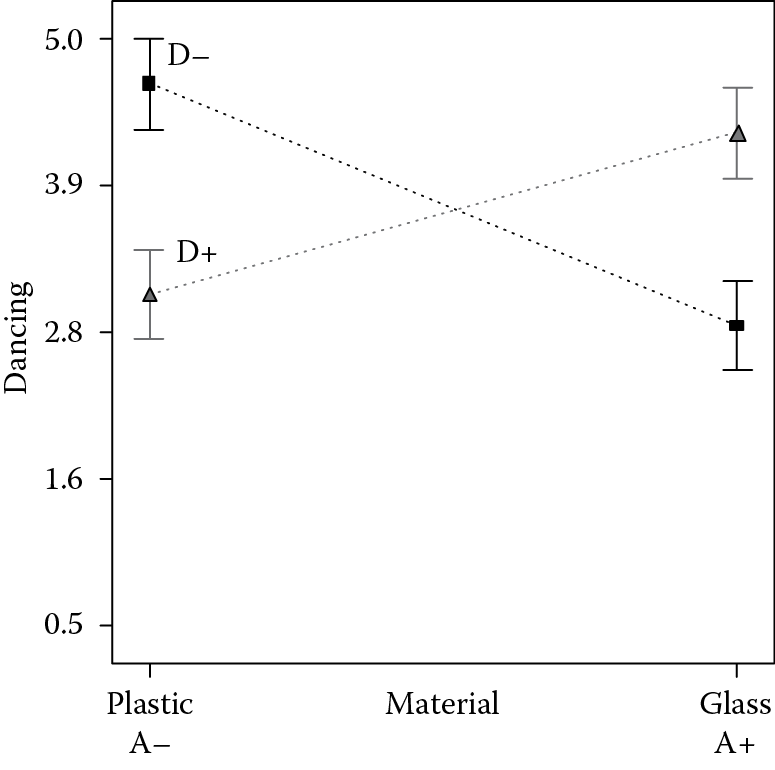
Discounting the CF interaction (liquid type versus object type) is not easy, but this new evidence clearly shows that the interaction between E and G is the most plausible, particularly since we now know that these two factors are present as main effects. Figure 6.6 shows the EG interaction.

It appears that the effect of cap (E) depends on the age of the object (G). When the object is stale (the G+ line at the bottom of Figure 6.6), twisting on the bottle cap (going from E– at left to E+ at right) makes little difference. However, when the object is fresh (the G– line at the top), the bottle cap quenches the dancing reaction. More experiments are required to confirm this interaction. One obvious way to do this is to conduct a full factorial on E and G alone. Other ideas on de-aliasing are presented after the next sidebar.

Single-Factor Foldover

Another simple way to de-alias a resolution III design is the “single-factor foldover.” Like a complete foldover, this requires a second block of runs, but in this variation of the general method, you change signs on only one factor. This factor and all its two-factor interactions become clear of any other main effects or interactions. To see how this works, go back to the original resolution III design on the dancing raisins. It makes sense to focus on the biggest effect: E (refer to Figure 6.1). The end result of the foldover on factor E (only) is a design with 16 runs in two blocks of eight. The resulting alias structure (main effects and two-factor interactions only) is shown in Table 6.5.

The combined design remains at resolution III because, with the exception of E, all main effects remained aliased with 2 two-factor interactions. Factor E is a resolution V, because the main effect is clear of troublesome aliases (anything less than a four-factor interaction), and the two-factor interactions are aliased only with three-factor or higher-order interactions. In the case of the dancing raisins, the single-factor foldover would have revealed that B was actually EG, not AD. On the other hand, factor G remains aliased with 2 two-factor interactions. You can’t win either way.

Choose a High-Resolution Design to Reduce Aliasing Problems

The best way to reduce aliasing problems is to run a higher resolution design in the first place by selecting fewer factors and/or a bigger design. For example, in the dancing raisin experiment, we would have prevented much confusion by testing the 7 factors in 32 runs (27-2). This option was discussed in the previous chapter on fractional factorials. It is a resolution IV design, but all 7 main effects and 15 of the 21 two-factor interactions are clear of other two-factor interactions. The remaining 6 two-factor interactions are shown in Table 6.6.

The trick is to label the likely interactors anything but D, E, F, and G. For example, knowing now that capping and age interact in the dancing raisin experiment, we would not label these factors E and G. If only we knew then what we know now.

Another option, one that requires no premonition, is to use a minimum-run resolution V (MR5) design (described in the appendix of this chapter). With just 30 runs, all main effects and two-factor interactions can be estimated.

Practice Problems

Problem 6.1

(Warning: The following story contains liberal doses of fantasy.) One of the authors became envious of the skating ability of his co-author. The “wannabe” skater secretly got together with a local manufacturer of in-line skates and borrowed the latest and greatest experimental gear. Bewildered by all the options, he decided to try various combinations at the local domed stadium, which opened its concourse to skaters when not in use for sporting events. The special skates would have to be returned fairly soon, so the wannabe skater set up a quick-and-dirty fractional factorial. If anything proved to be statistically significant, the result would be a faster time around the track (and, of course, some ego gratification). The experimenter knew that aliasing of effects would obscure a true picture of what really enhanced speed, but he anticipated that this could be figured out later through follow-up designs using the foldover method. Table 6.7 shows the initial design, a 27-4 resolution III fractional factorial, and the resulting times around the track.

Here is more background on the factors and levels to help you interpret the outcome:

1. Pad goes inside skate to elevate the heel: Out (−), In (+)
2. Bearing constructed either from old material (−) or new high-tech alloy (+)
3. Gloves made specially for in-line skating to protect wrists: On (−), Off (+)
4. Helmet fits with logo to back (−) or front (+): Can’t tell which is correct, so try both and ignore laughs when wrong
5. Wheels can be made of hard (−) or soft (+) polymer
6. Covers go on wheels to make them look faster: On (−), Off (+)
7. Neon lighting (from generator on skates) for night-time use: Off (−), On (+)

Analyze the data to see if any of these factors appear to be significant. Do the results make sense? Could the real answer be disguised by an alias? (Suggestion: Refer to Table 6.3. Use the software provided with the book. Create a two-level factorial design for 7 factors in 8 runs and sort the resulting layout by standard order, then enter the time data from Table 6.7. Do the analysis as outlined in the factorial tutorial that comes with the program.)

Problem 6.2

This is a continuation of the skating saga from Problem 6.1. Rolling right along, the experimenter decided to do a complete foldover on the initial design. Table 6.8 shows the factor levels and results for this follow-up design.

Add these data to the design from Problem 6.1 and analyze it as a second block of data. Do any of the significant model terms turn out to be interactions rather than main effects? Remember that the foldover upgrades the resolution III design to resolution IV, but interactions may still be aliased with other interactions. If interactions do appear, do they make more sense than the aliased alternatives? (Suggestion: Use the software provided with the book. Look for a data file called “6-P2 Skate2,” open it, then do the analysis. View the aliased interactions and try substitutions. Graphically compare the alternatives in a similar manner to that outlined for the dancing raisin case.)

Appendix: Minimum-Run Designs for Screening

In the presence of two-factor interactions, only designs of resolution IV (or higher) can ensure accurate screening. If you are limited by time, materials, or other experimental resources, in most cases (other than eight factors), modern “minimum run” resolution IV (MR4) designs offer savings in runs over the equivalent standard two-level fractional factorial design (2k-p). A nine-factor MR4 design, for example, requires only 18 runs, far fewer than the 32 runs needed for a standard 2k-p. In general, the MR4 designs require only two times the number of factors (2k). Table 6.9 details a minimum-run screening design on six factors that a biotechnologist ran on a fermentation process (from: Mark Anderson and Patrick Whitcomb, October 2006, Chemical Processing. Online at www.chemicalprocessing.com/articles/2006/166/).

What you do as a result of running such a screening design depends on the statistical analysis of the effects:

Scenario 1: Nothing significant. Look for other factors that affect your response(s).

Scenario 2: Only main effects significant. Change these factors to their best levels.

Scenario 3: Two-factor interaction(s) significant. De-alias by performing a semifoldover.

By following this strategy you will increase your odds of uncovering breakthrough main effects and interactions at a relatively minimal cost in experimental runs.

The development of minimum-run, two-level factorial designs has gone to the next level with resolution V “characterization” designs such as the MR5 (minimum-run resolution five) shown in Table 6.10 for six factors in only 22 runs. The following boxed text provides some background and a reference for more details on the new class of MR5 designs.