Chapter 7

General Multilevel Categoric Factorials

Invention is discernment, choice. … The useful combinations are precisely the most beautiful.

Henri Poincaré

In Chapter 2, we showed how to perform simple comparative experiments on individual factors with any number of levels. In the chapters that followed, we shifted to experiments with multiple factors, but restricted to just two levels. You might find it helpful at this point to revisit the flowchart in the Introduction, which directs you to the various types of experiments covered in this book. Your decision on which designs will prove most useful depends on:

• Number of factors
• Number of levels
• Nature of factors: numerical or categorical, process or mixture.

Quite often, you may be confronted with a number of categorical alternatives, such as three suppliers (A versus B versus C), as well as other categorical factors that could interact with the first. A good example of this is what happens when brewing several varieties of coffee with a number of flavoring additives—a second categorical factor. A simple solution to this problem is to run all combinations of all factors. Unfortunately, this “general factorial” design is not very popular and with good reason:

1. The number of combinations becomes excessive after only a few factors. It may be possible to perform fractional designs, but except for special cases documented in the literature, you must resort to computer-aided selection via matrix-based methods. This goes well beyond the scope of DOE Simplified, but see the boxed text on optimal design at the end of Chapter 6 for some clues.
2. Each design is unique to the given situation, with many possible levels for the specified varying numbers of factors. Therefore, you may not find a template or example that you can follow for design and analysis.
3. Due to the already large number of combinations, general factorials for three or more factors are often done without replication. Because no pure error is available, you must assume that highest-order interactions are insignificant and build your analysis of variance (ANOVA) from this basis.
4. Predictive models for categorical factors must be coded in a nonintuitive manner.

To avoid these complications, stick with simple comparisons and two-level factorials. In the coffee example cited above, for example, you can begin by screening several varieties of coffee via a one-factor, simple-comparative taste test. After eliminating all but the top two varieties, combine these with your two favorite flavor additives, with additional factors at two levels, such as brewing temperature low versus high, in a standard factorial. It is important to note, however, this simplistic approach to experiment design may overlook critical interactions that will be revealed in a general factorial design. For example, perhaps one of the coffee varieties eliminated early on may have worked really well if paired with a particular flavor additive. Therefore, rather than taking the simpler route, we will detail the more comprehensive general factorial choice in the following case study.

Putting a Spring in Your Step: A General Factorial Design on Spring Toys

A coiled spring, made to specific dimensions (see boxed text below), will gracefully “walk” down an incline. The most obvious factor affecting speed is the degree of incline, which must be between 20 and 40 degrees. If the incline is too shallow, the coil will not move. Too steep an incline causes the coil to tumble or roll out of control. Friction also plays a role. During our coiled-spring experiment, after observing slippage on bare wood, we added a high-friction rubber mat for the walking surface. Many other variables are associated with the construction of the coil, such as the spring constant, mass, diameter, and height.

Several varieties of coiled springs are made by Poof-Slinky, including the Slinky and the smaller Slinky Junior. They come in traditional metal or styrene-butadiene plastic. The first two “bent” springs (resting in curved formation) shown in Figure 7.1 (starting from bottom left and then going on up the picture) are a metal Slinky in traditional size and a plastic Slinky Junior. We also looked at a larger plastic Giant Slinky (shown in the hands of tester in Figure 7.1), but it walked too slowly and frequently stopped.

Two additional generic plastic spring toys (the coiled ones in the picture) were tested. The smaller of these walked too fast for valid comparison to the Slinky brands. That left three coiled spring toys to test at two inclines in a full factorial experiment. We replicated each of the six combinations (3 * 2) in a completely randomized test plan. The 12 results are sorted by standard order in Table 7.1.

The response is time in seconds for the springs to walk a four-foot inclined plank. The two results per cell represent the replicated runs. As noted earlier, these runs were performed at random, not one after the other, as shown. Therefore, the difference in time reflects the variations due to setting of the board, placement of the coil, how the operator made it move, and so forth. The ANOVA is seen in Table 7.2. Procedures for calculating the sums of squares are provided in referenced textbooks and encoded in many statistical software packages.

Look first at the probability value (Prob > F) for the model. Recall that we consider values less than 0.05 to be significant. (Reminder: A probability value of 0.05 indicates a 5% risk of a false positive, i.e., saying something happened because it was influenced by a factor when it actually occurred due to chance. An outcome like this is commonly reported to be significant at the 95% confidence level.) In this case, the probability value of 0.0056 for the model easily passes the test for significance, falling well below the 0.05 threshold. Because we replicated all six combinations, we obtained six degrees of freedom (df) for estimation of error. This is shown in the line labeled Residual. The three effects can be individually tested against the residual. The result is an unexpectedly large interaction (AB). This is shown graphically in Figure 7.2.

The two Slinky springs behaved as expected by walking significantly faster down the steeper incline (B+). However, just the opposite occurred with the generic plastic spring. It was observed taking unusually long, but low steps down the shallow slope, much like the way the comedic actor Groucho Marx slouched around in the old movies. While it didn’t look very elegant, it was fast. On the steep slope, the generic spring shifted into the more pleasing, but slower and shorter high-step, like the Slinky toys.

How to Analyze Unreplicated General Factorials

The example shown above involved only six combinations for the full factorial, so doing a complete replicate of the design was feasible. When you add a third factor, the cost of replication goes up twofold or more, depending on how many levels you must run. In this case, it’s common practice to assume that interactions of three or more factors are not significant. In other words, whatever effects you see for these higher order interactions are more than likely due to normal process variability. Therefore, these effects can be used for estimating error. Other insignificant interactions also may be pooled as error in much the same way as with two-level factorials discussed earlier in this book. A new example based on the same toys as before illustrates this concept in a way that keeps things simple and fun.

Before conducting the earlier case study on the springs, we rejected two abnormal toys:

• A larger one: The “original plastic Slinky”
• A smaller one: A generic plastic variety

In this new example, we will go back and test these two springs, along with two from the earlier test, excluding only the generic plastic toy. The factor of incline will be retained at two levels. A third factor will be added, which is whether an adult or a child makes the springs walk. The resulting 16 combinations (4 * 2 * 2) are shown in Table 7.3, along with the resulting times.

The impact of the three main effects and their interactions can be assessed by analysis of variance. In general factorials like this, it helps to view a preliminary breakdown of sum of squares (a measure of variance) before doing the actual ANOVA. In many cases you will see that some or all of the two-factor interactions contribute very little to the overall variance. These trivial effects then can be used as estimates of error, in addition to the three-factor or higher interactions already destined for error. Table 7.4 provides the sum of squares, degrees of freedom, and the associated mean squares for the time data from the experiment on spring toys.

The main effect from factor A ranks first on the basis of its mean square. The main effect of B comes next. The other main effect, from factor C, contributes relatively little to the variance. Continuing down the list, you see fairly low mean squares from each of the 3 two-factor interactions (AB, AC, BC). Finally, you get to the three-factor interaction effect ABC, which (as stated earlier) will be used as an estimate of error. Because none of the other interactions caused any larger mean square, these also will be thrown into the error pool (labeled “Residual” in the ANOVA). The rankings in terms of mean square (the last column in Table 7.4) provide support for this decision. Although it appears to be trivial, the C term will be kept in the model because it is a main effect. The resulting main-effects-only (A, B, C) model is the subject of the ANOVA shown in Table 7.5.

The model passes the significance test with a probability of less than 0.001 (>99.9% confidence). As expected, A and B are significant, as indicated by their probability values being less than 0.05. By this same criterion, we conclude that the effect of factor C (child operator versus adult operator) is not significant. The probability is high (0.3626) that it occurred by chance. In other words, it makes no difference whether the adult or the child walked the spring toy. The effect of A—the type of spring toy—can be seen in Figure 7.3, the interaction plot for AB. (Normally we would not show an interaction plot when the model contains only main effects, but it will be helpful in this case for purposes of comparison.)

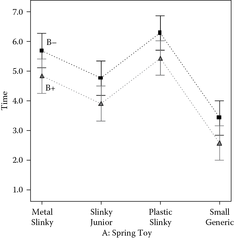
Compare Figure 7.3 with Figure 7.2. Notice that in this second design the lines are parallel, which indicates the absence of an interaction. The effects of A and B evidently do not depend on each other. You can see from Figure 7.3 that the shallower incline (B−) consistently produced longer predicted times. The main-effect plot in Figure 7.4 also shows the effect of B, but without the superfluous detail on the type of spring.

As expected, the spring toys walked faster down the steeper slope.

This example created a template for general factorial design. Setup is straightforward: Lay out all combinations by crossing the factors. With the aid of computers, you can create a fractional design that fits only your desired model terms, but this goes beyond the scope of the current book. Check your software to see if it supports this “optimal design” feature. If you don’t include too many factors or go overboard on the number of levels, you might prefer to do the full factorial. Replication is advised for the two-factor design, but it may not be realistic for larger factorials. In that case, you must designate higher-order interactions as error and hope for the best.

If at all possible, try to redesign your experiment to fit a standard two-level factorial. This is a much simpler approach. Another tactic is to quantify the factors and do a response surface method design (see above boxed text).

Practice Problems

Problem 7.1

Douglas Montgomery describes a general factorial design on battery life (see Recommended Readings, Design and Analysis of Experiments, 2012, ex. 5.3.1). Three materials are evaluated at three levels of temperature. Each experimental combination is replicated four times in a completely randomized design. The responses from the resulting 36 runs can be seen in Table 7.6.

Which, if any, material significantly improves life? How are results affected by temperature? Make a recommendation for constructing the battery. (Suggestion: Use the software provided with the book. First do the tutorial on general factorials that comes with the program. It’s keyed to the data in Table 7.6.)

Problem 7.2

One of the authors (Mark) lives about 20 miles due east of his workplace in Minneapolis. He can choose among three routes to get to work: southern loop via freeway, directly into town via stop-lighted highway, or northern loop on the freeway. The work hours are flexible so Mark can come in early or late. (His colleagues frown on him coming in late and leaving early, but they don’t object if he comes in early and leaves late.) In any case, the time of Mark’s commute changes from day to day, depending on weather conditions and traffic problems. After mulling over these variables, he decided that the only sure method for determining the best route and time would be to conduct a full factorial replicated at least twice. Table 7.7 shows the results from this general factorial design. The run order was random.

Analyze this data. Does it matter which route the driver takes? Is it better to leave early or late? Does the route depend on the time of departure? (Suggestion: Use the software provided with the book. Look for a data file called “7-P2 Drive,” open it, then do the analysis. View the interaction graph. It will help you answer the questions above.)

Appendix: Half-Normal Plot for General Factorial Designs

Stat-Ease statisticians developed an adaptation of the half-normal plot—so very handy for selecting effects for two-level factorial designs—for similar use in the analysis of experimental data from general factorial designs. This is especially useful for unreplicated experiments, such as the second one done on spring toys. Notice, for example, how the main effect of factor A (and to some extent B) stands out in Figure 7.5.

The other (unlabeled) five effects, C, AB, AC, BC, and ABC, line up normally near the zero-effect level and, in all likelihood, they vary because of experimental error (noise). This graphical approach provides a clear signal that A and B ought to be tested via the analysis of variance (ANOVA) for statistical significance. In this case, having access to this half-normal plot (not yet invented when the initial baseline experiment was performed) would have saved the trouble of testing the main effect of factor C for significance (Table 7.5). For details, see the proceeding for “Graphical Selection of Effects in General Factorials” by Patrick J. Whitcomb and Gary W. Oehlert. Paper submitted for the 2007 Fall Technical Conference of the American Society for Quality (ASQ) and American Statistical Association (ASA), October.