Chapter 5

Fractional Factorials

Believe nothing and be on your guard against everything.

Latin Proverb

The full-factorial approach to experimentation covers all combinations of factors, providing valuable information on interactions. However, the number of experimental runs increases rapidly, even if you test the factors at only two levels each. Fortunately, by cutting back to a “fractional factorial,” you may find it possible to study more factors within a given experimental budget. Table 5.1 shows how few runs we suggest you pare back to for four to seven factors (see Appendix 2 for details on layout.). These particular designs are especially good for “screening” the main effects of many factors in search of the vital few or more in-depth “characterizing” for possible two-factor interactions. For reference, we show the number of main effects and two-factor interactions (2 fi). A minimal experiment for screening requires at least two times the number of runs as the number of factors, e.g., 8 runs for 4 factors. An efficient fraction for characterization contains at least this many runs plus one more for estimating the overall average, but no more. The five-factor, 16-run half fraction is an ideal example—a “minimum run” design for resolving main effects and 2 fis. Unless runs come free, consider choosing a fractional factorial for four or more factors.

We hope this whets your appetite, because we will soon get into the nitty-gritty of fractional factorial design. You will learn that there is a price to pay in the form of “aliasing” effects and, due to the reduction in runs, an inevitable power loss. The more you know about this the better, because conducting fractional factorials is like playing with fire. It’s a powerful tool that can burn you if not handled carefully.

Example of Fractional Factorial at Its Finest

Let’s begin with an example of a very safe fractional factorial: five factors at two levels each, done in 16 runs (a half fraction). This data comes from an actual experiment on an uncooperative grass trimmer, commonly known as a weedwacker. A one-cylinder engine that runs on a mixture of gasoline and oil powers the weedwacker (Figure 5.1). Perhaps you have become frustrated trying to start small engines such as this one.

The weedwacker engine features a manual starter (pull cord), and its performance is largely a function of three controls: primer pump, choke, and gas. Before starting the engine, you must first give the primer several pumps, choke the air intake, and pull the starter cord several times. To start the engine, the choke must be open. Table 5.2 lists the tested factors and levels.

It would require 32 runs to perform all the combinations of these five factors. This full, two-level factorial would reveal 31 effects: 5 main effects, 10 two-factor interactions, 10 three-factor interactions, 5 four-factor interactions, and 1 five-factor interaction. Interactions of three or more factors are highly unlikely in an engine or any other system. Moreover, the principle of sparsity of effects states that only 20% of the main effects and two-factor interactions are likely to be significant in any particular system. If this is true, then only about three effects will be significant, which leaves 28 effects for estimation of error; far more than necessary. Therefore, a full factorial on five factors (or more) will waste much of its effects on unneeded estimates of error.

A properly constructed half fraction (16 runs) estimates the overall mean, the 5 main effects, and the 10 two-factor interactions. The design for the weedwacker, constructed by standard methods, is shown in Table 5.3. Experiments are listed in standard (Std) order, not randomized run order. Factors are shown in coded format. The response (Y) is pulls needed to start the engine.

You can use this as a template for your own experiment on five factors. Notice that the first four factor columns form a full factorial with 16 runs. The fifth factor column (E) is the product of the first four columns (ABCD). Check it out. This and many other fractional designs can be generated via statistical software or from tables in referenced textbooks on DOE. We will give you more clues on their construction later on in this section.

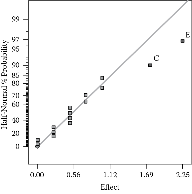
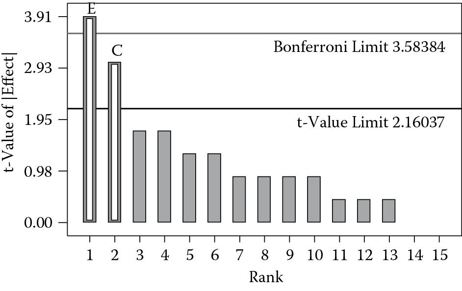
The half-normal plot of effects (Figure 5.2) reveals two large main effects: factors E and C. The Pareto plot in Figure 5.3 supports the hypothesis that these two effects are the vital few versus the others being the trivial many. Do not forget, however, that E was constructed from ABCD and that these two effects are, therefore, aliased. The effect of C is also aliased with a four-factor interaction: ABDE. (Check this out by multiplying the appropriate columns and comparing signs.) Four-factor interactions are not plausible, so we will ignore these aliases. This assumption follows the generally accepted practice of statisticians. However, you must keep in mind that you rarely get something for nothing; fractional factorials save on runs but they produce aliases, which can be troublesome. (See the next section, (Potential Confusion Caused by Aliasing in Lower Resolution Factorials), for more on this subject.)

The F-test on the resulting model was significant at a 99.9% confidence level. Residual analysis showed no abnormalities. Figure 5.4 shows the four combinations of the two significant factors. The best combination (least number of pulls) occurs at low C and high E at the upper left of the square plot.

None of the other factors created a statistical significant effect, so for ease of operation they were set at their most advantageous level. The ideal procedure for minimizing pulls is:

• Prepare engine with three primer pumps and three pulls at 100% choke with 0% gas
• Start at 0% choke at 100% gas

In the confirmation trial, the engine started immediately on the first pull.

Potential Confusion Caused by Aliasing in Lower Resolution Factorials

You may be wondering whether the application of fractions to factorial design appears to be too good to be true, and, as noted above, this is a valid point to consider. The price you pay when you cut down the number of runs is the aliasing of effects. This is measured by the “resolution” of the fractional factorial. The half-fractional design on the five weedwacker factors is a resolution V (the resolution is represented by Roman numerals), which indicates aliasing of at least one main effect with one or more four-factor interaction(s), and/or at least one two-factor interaction(s) with one or more three-factor interaction(s). Think of these as relationships of 1 with 4 and 2 with 3, both of which total to 5. As detailed in the sidebar on A Handy Way To Put Your Finger On The Concept Of Resolution, you can figure this out with your fingers!

As you might expect, as resolution decreases, alias problems increase. Let’s go to a worst-case scenario for two-level factorials—a resolution III design, which we will demonstrate by revisiting the popcorn case from Chapter 3. The unshaded rows in Table 5.4 represent a half-fraction of the original data. It was created by eliminating the minus ABC runs (shaded in the table).

Can you see any problems with the resulting pattern of pluses and minuses in the clear rows?

At first glance, the design looks good, with a nicely balanced pattern for the main effects of A, B, and C. However, upon closer inspection, notice that each effect column has an identical twin in terms of the pattern of pluses and minuses (shown below in parentheses) that you see from top to bottom in the clear rows:

A = BC (+, –, –, +)

B = AC (–, +, –, +)

C = AB (–, –, +, +)

These equalities are called confounding relationships, or aliases. The most troublesome of these aliases involves the interaction BC. Recall that the full factorial revealed this to be a significant effect. However, as shown above, the half fraction attributes the BC effect to A, which is completely misleading. The effect labeled “A” is actually the combination of A and BC, which can be expressed mathematically as: A = A + BC. (To check this equation, observe that the effects of A and BC from the full factorial are –1.0 and –21.5, respectively, which sum to the value of –22.5 for A in the half fraction.)

Finally, notice that the last effect column, ABC, displays only plus symbols in the clear rows of Table 5.4. Because there is no contrast in the signs, this effect can no longer be estimated. The calculated value of 64.75, labeled as an effect, is actually an estimate of the overall mean or intercept.

You can now see the downside to creating a fractional design: aliasing of effects. In this case, we cut a full factorial to a half fraction by eliminating the negative ABC rows. The resulting loss of information about the ABC effect is not critical, because three-factor interactions rarely occur. However, you should be very concerned about the aliasing of main effects with two-factor interactions. Statisticians consider such a design to be resolution III, the lowest possible for standard fractional two-level factorials. We recommend that you avoid resolution III designs if at all possible, because if your system contains any interactions, the true cause will be disguised by the aliasing. However, because shortcuts must be taken from time to time under extreme deadlines, we will provide more details on resolution III designs and show how to “de-alias” them in the next chapter.

So far we have shown examples of resolution V (good) and resolution III (bad). Let’s fill the gap with a resolution IV design, which represents a reasonable compromise between minimal runs and maximum information on the main effects. Table 5.5 shows a complete matrix of effects for four factors. The rows where ABCD is minus are shaded. The remaining rows form the half fraction. Look over the resulting columns very carefully, ignoring the gray cells. Can you see the aliases? (Hint: Start in the middle, at AD–BC and work outward.)

In this case, every main effect is aliased with a three-factor interaction, and all the two-factor interactions are aliased with each other, so this design is resolution IV.

Assuming that three-factor interactions are unlikely, you can rely on main effect estimates from resolution IV designs, but don’t jump to any conclusions on any significant two-factor interactions. For example, if AB shows significance, it might really be due to CD, which changes in exactly the same way: +, +, –, –, –, –, +, + from top to bottom, clear rows only. We will show you how to escape from this trap in the next chapter of the book.

Not all resolution IV designs are the same. Some have only a few two-factor interactions aliased with each other. For example, the seven factors in 32-run design (1/4 fraction) shown on Table 5.6 are listed as a resolution IV, but only six of the two-factor interactions (those involving D, E, F, and G) are actually aliased (DE = FG, DF = EG, and DG = EF). The other 15 two-factor interactions are aliased only with three-factor or higher interactions. Therefore, you would be wise to assign factors that are least likely to interact with the labels D, E, F, or G, and those factors most likely to interact with A, B, and C.

On the other hand, you might be tempted to cut back to only 16 runs for the seven-factor design, a 1/8 fraction. After all, as shown in Table 5.6, it too is resolution IV. However, as you can see from the alias structure shown in Table 5.7, no matter how you do the labeling, even one active interaction may cause confusion. For example, let’s say that only C and D interact in a particular system. This interaction (CD) will be mislabeled as AG due to the aliasing. It should be apparent by now that you must investigate the alias structure for anything less than resolution V designs. You will find the details on construction of optimal fractions and their alias structures from referenced textbooks by Box et al. and Montgomery, found in Recommended Readings. Good DOE software also will set up the appropriate fraction and supply information on the specific aliases of your chosen design.

Plackett–Burman Designs

The standard two-level designs, which we recommend, provide the choice of 4, 8, 16, 32, or more runs, but only for powers of 2. In 1946, Robin Plackett and J. P. Burman invented alternative two-level designs that are multiples of 4. The 12-, 20-, 24-, and 28-run Plackett–Burman designs are of particular interest because they fill gaps in the standard designs. Unfortunately, these particular Plackett–Burman designs also have very messy alias structures. For example, the 11 factor in the 12-run choice, which is very popular, causes each main effect to be partially aliased with 45 two-factor interactions. In theory, you can get away with this if absolutely no interactions are present, but this is a very dangerous assumption in our opinion.

Of course, you could cut down the number of factors in a given Plackett–Burman, but the alias structure may not be optimal. Assuming that your software provides such information, be sure to look at the alias structure before doing your experiment.

Overall, because of the unexpected aliasing that occurs with many Plackett–Burman designs, we recommend that you avoid them in favor of the standard two-level designs. However, if you must use Plackett–Burman, consider following up with a second set of runs, but not an exact replicate of the initial block. In the next chapter, we show how to do a “foldover” that doubles the number of runs in a way that increases the resolution of highly aliased Plackett–Burmans and standard fractional factorials.

Irregular Fractions Provide a Clearer View

At this point, you have seen several options for the standard two-level design, which apply fractions that are negative powers of 2 (1/2, 1/4, etc.). However, it is possible to use other “irregular” fractions and still maintain a relatively high resolution. A prime example of this is the three-quarter (3/4) replication (rep) for four factors (the first design in Table 5.1). It can be created by identifying the standard quarter fraction, and then selecting two more quarter fractions. This design contains only 12 runs, yet it estimates all main effects and two-factor interactions aliased only by three-factor or higher interactions, thus making it a viable alternative to the 16-run full factorial. (Details on this and other designs of the like can be found in Peter John’s Statistical Design and Analysis of Experiments (see Recommended Readings).) In Table 5.8 is an example of this irregular fraction with four factors in 12 runs.

In the 1990s, the authors frequently presented computer-intensive workshops on DOE in corporate training rooms equipped with RGB (red-green-blue) projectors. Students often found it difficult to read the projected statistical outputs. To improve readability, co-author Mark investigated four factors at two levels as shown in Table 5.8. The assignment of minus versus plus levels for the categorical variables (B, C, D) is completely arbitrary.

During one of our workshops, students worked together on the exercise. Mark (the instructor) displayed a column of numbers in random order. One student transcribed the data from top to bottom while the other timed it. The actual experiment was performed by many students. By treating each student as an individual block, Mark eliminated variability caused by differing distance from the screen and reading ability. However, to keep it simple, the results are shown as one block of data. Table 5.9 provides the complete design with the resulting readability measured in seconds. Shorter times are desired.

The four main effects (A, B, C, D) can be calculated in the usual way by contrasting the average of the plus values with the average of the minus values for the associated response (symbolized by Y). For example, the main effect of factor A is

$\begin{array}{c}Effec{t}_A=\frac{{\displaystyle \sum Y_{A+}}}{n_{A+}}-\frac{{\displaystyle \sum Y_{A-}}}{n_{A-}}=\frac{39+27+31+28+30+19}{6}-\frac{52+42+37+57+52+47}{6}\\ =\text{2}9.00-47.83=-18.83\end{array}$

In other words, with a font size of 18 points, students read the projected display 18.83 seconds faster (on average) than with a font size of 10 points. In this case, the bigger the better. The effect of A (font size), in absolute value, stands out on the half-normal plot (Figure 5.5).

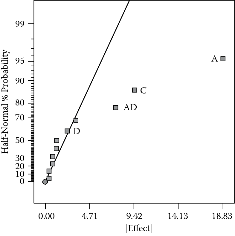
The main effect of C (background) and the interaction AD (font size times lighting) also fall off the normally distributed line of near-zero effects. As usual, we did not label any of the smaller, presumably insignificant effects, with one exception: D. For statistical reasons, which will be discussed later, this main effect must be chosen to support the choice of the AD interaction.

The sharper-eyed (and particular) readers among you may be wondering why 11 points are displayed on Figure 5.5. Ten of the points show estimates of the effects of interest: four main effects plus 6 two-factor interactions. The eleventh point is a three-factor interaction, which provides an estimate of error. Remember that we started with 12 runs. We used one bit of information (degree of freedom) to estimate the overall mean. That leaves us with 11 bits of information, of which 10 get used for designed-for effects, with one left over to use as an estimate of error. There is no reason to throw away information if it can be used to serve some purpose.

Table 5.10 shows the analysis of variance for the RGB data.

You may still be curious as to why we include factor D in the model because it is not significant in the analysis of variance (ANOVA). The factor was chosen to support the significant AD interaction, thus maintaining model “hierarchy” (see Preserving Family Unity below).

Although factor D is not significant on its own, it does have an effect on readability, but only in conjunction with factor A. This becomes very clear when you look at the interaction graph in Figure 5.6 (produced with other factors averaged).

If you split the differences from left (D−) to right (D+), you get a nearly flat line, indicating that D has no effect, thus explaining why it falls on the near-zero effect line shown in the half-normal plot. However, to say that D has no effect makes no sense. Factor D does affect the response, but it depends on the level of Factor A (font size). When A is low (−), increasing D increases the response. However, when A is high (+), increasing D decreases the response. In either case, factor D does cause an effect. Therefore, it should not be excluded.

From a practical perspective, the upper line on the AD interaction tells us that students find it more difficult to read the RGB screen when the font size is small (A−) with the lights turned on (D+). The lower line shows that when font size is large enough, it doesn’t matter if you turn on the lights; in fact, the readability results actually improved. This was a very desirable outcome, because it allowed students to read their notes while viewing the RGB screen.

One other effect stood out on the half-normal plot: the main effect of C (background). As you can see in Figure 5.7, the readability improves (lower the time, the better) at the high level of this factor, which represents the background set to white.

Finally, we put all three of the significant factors together in the form of the cube plot shown in Figure 5.8. It shows the best result (19 seconds) at the right, back, and upper corner where all factors are set at their high levels.

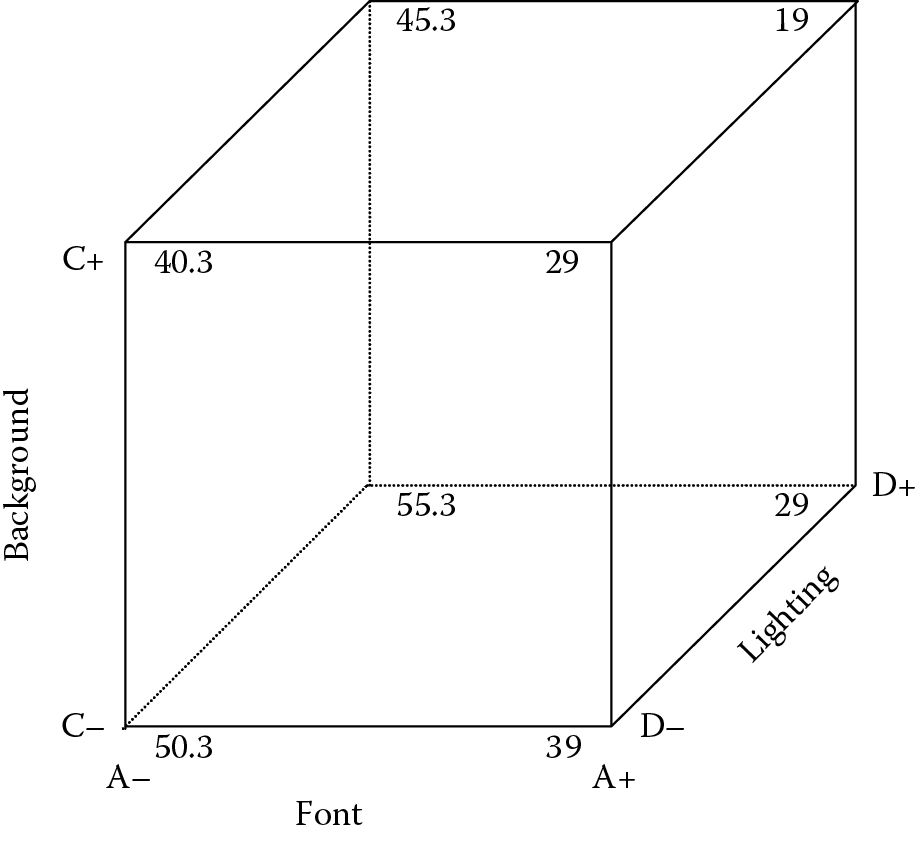
Note that B (font style) was not significant, so either style can be chosen. One author likes Arial and the other Times New Roman, but neither is likely to affect readability. Thankfully, projection technology has improved far beyond RGB to a point where its brightness, contrast, and resolution make it far easier to read all the numbers we put up on the screen.

Practice Problem

Problem 5.1

An injection molder wanted to gain better control of part shrinkage. The experimenter set aside two parallel production lines for a study of seven factors (Table 5.11).

All possible combinations of these factors require 128 runs, but only 32 of these were actually done: a 1/4 fraction. This DOE is symbolized mathematically as 27-2. It is one of the recommended fractional factorial designs for screening (see Table 5.1). From the 32 runs, you can get information on all the main effects and nearly all two-factor interactions. Table 5.12 shows the design matrix in terms of coded factor levels, and the results for shrinkage.

Notice that the experiment is divided into two blocks of 16 runs in a standard way that preserved the greatest possible information on main effects and interactions. The experimenters then ran the DOE on the two parallel lines, greatly reducing the time needed to generate the data, as well as providing information on machine-to-machine variation.

The blocking does cause further loss of information in the form of additional aliasing (revealed by statistical DOE software):

[Block 1] = Block 1 + CDG + CEF + ABDE + ABFG

[Block 2] = Block 2 – CDG – CEF – ABDE – ABFG

The loss of the three-factor and higher interactions didn’t cause much worry. The experimenters also carefully reviewed the alias structure (see Appendix 2.4) before assigning labels. By labeling the most likely interactors—booster pressure and moisture—as C and D, they avoided deliberate aliasing of this potential effect with other two-factor interactions.

Analyze the data. Look for conditions that minimize and/or stabilize shrinkage. Remember to check the significant factors against the alias structure.

(Suggestion: Use the software provided with the book. Look for a data file called “5-P1 Molding” and open it. Otherwise, create the design by choosing a factorial for 7 factors in 32 runs with 2 blocks and enter the data (from Table 5.12) in standard order. Then do the analysis as outlined in the factorial tutorial that comes with the program.)