
4
S-weighted Instrumental Variables
This chapter deals with two problems – with the situation when the orthogonality condition is broken and with the problem when an atypical data set contains a significant amount of information in a group of good leverage points but includes also a “troublesome” group of outliers.
Several robust methods were recently modified in order to overcome problem with the broken orthogonality condition, employing typically the idea of instrumental variables. In an analogous way, modified S-weighted estimator is also able to cope with broken orthogonality condition. We prove its consistency and we offer a small pattern of results of simulations.
It is believed that the bad leverage points are a more challenging problem in identification of underlying regression model than outliers. We show that sometimes outliers can also represent an intricate task.
4.1. Summarizing the previous relevant results
The median is the only classical statistic that is able to cope with high contamination, even 50%, and to give reasonable information about the location parameter of a data set. When Peter Bickel (Bickel 1975) opened the problem of possibility to construct an analogy of median in the framework of regression model, that is, an estimator of regression coefficients with 50% breakdown point, nobody had an idea how long and painful way to the solution we would have to go.
It seemed several times that we had achieved solution but finally always a bitter disappointment arrived. For instance, as the median is in fact the 50% quantile, we hoped that Koenker and Bassett’s regression quantiles were the solution (Koenker and Bassett 1978). However, results by Maronna and Yohai (1981), establishing the maximal value of breakdown point of M-estimators, ruined our dreams.
By proposing the repeated median, Siegel (Siegel 1982) has broken this long years lasting nightmare. But only proposals of the least median of squares (LMS) and the least trimmed squares (LTS) by Rousseeuw (Rousseeuw 1983, 1984) and (Hampel et al. 1986) brought feasible methods. In fact, he “rediscovered” the power of such statistical notion as the order statistics of (squared) residuals (see Hájek and Šidák 1967). Unfortunately, at those days we have not at hand a proper tool for studying the asymptotic properties of these estimators (the proof of consistency of LTS arrived after 20 years from its proposal (see Víšek 2006) and this technical problem was (except of others) an impulse for proposing S-estimator (Rousseeuw and Yohai 1984) with an immediately available proof of consistency and the simultaneous preservation of high breakdown point.
The algorithms for all these estimators were also successfully found. For LTS, it was based on repeated application of algorithm for the ordinary least squares and it was so simple that it was not published (as such, see Víšek 1990) until the moment when an improvement for large data set became inevitable (Číek and Víšek 2000, Hawkins 1994, Hawkins and Olive 1999). The algorithm for the S-estimator was a bit more complicated but feasible (see Campbell and Lopuhaa 1998).
Nevertheless, results by Hettmansperger and Sheater (1992), although they were wrong (due to the bad algorithm they used for LMS – for efficient algorithm, see Boček and Lachout 1993), they warned us that the situation need not be so simple as we had assumed. It led to a return to the order statistics of squared residuals and to the proposal of the least weighted squares (LWS) in Vsek (2000). It profited from extremely simple algorithm, basically the same as the algorithm for LTS (see Víšek 2006b), however, the study of its properties was tiresome and clumsy (see Víšek 2002). A significant simplification came with generalization of Kolmogorov–Smirnov result for the regression scheme (see Víšek 2011a), together with the fact that the rank of given order statistic is given by the value of empirical distribution function of these order statistics at given order statistic (see Víšek 2011b). It opened a way for defining an estimator covering all above-mentioned estimators as special cases – S-weighted estimator – and to describe its asymptotics (see Víšek 2015, 2016).
Due to the character of data in the social sciences, we can expect that the orthogonality condition is frequently broken. That was the reason why there are several attempts to modify the robust methods to be able to cope with the broken orthogonality condition, similarly as the ordinary least squares were “transformed” into the instrumental variables (e.g. Carroll and Stefanski 1994, Cohen-Freue et al. 2013, Desborges and Verardi 2012, Heckman et al. 2006, Víšek 1998, 2004, 2006a,b, 2017, or Wagenvoort and Waldmann 2002). This chapter offers a similar modification of the S-weighted estimator, which is able to cope with the broken orthogonality condition (S-weighted instrumental variables).
At the end of chapter, we answer to the problem whether the leverage points represent always more complicated problem than outliers. And the answer is bit surprising.
4.2. The notations, framework, conditions and main tool
Let N denote the set of all positive integers, R the real line and Rp the p-dimensional Euclidean space. All random variables are assumed to be defined on a basic probability space (Ω, A, P ). (We will not write – as the mathematical rigor would ask it – the random variable as X(ω) (say) but sometimes by including (ω) we emphasize the exact state of things.) For a sequence of (p + 1)-dimensional random variables ![]() for any
for any ![]() and a fixed
and a fixed ![]() the linear regression model given as
the linear regression model given as
will be considered. (It is clear that the results of paper can be applied for the panel data – the model [4.1] will be used to keep the explanation as simple as possible.) We will need some conditions on the explanatory variables and the disturbances.
CONDITION C1.– The sequence ![]() is sequence of independent p + 1-dimensional random variables (r.v.’s) distributed according to distribution functions
is sequence of independent p + 1-dimensional random variables (r.v.’s) distributed according to distribution functions ![]() where
where ![]() is a parent d.f. and
is a parent d.f. and ![]() Further,
Further, ![]() ei = 0 and
ei = 0 and
We denote Fe|X(r|X1 = x) as the conditional d.f. corresponding to the parent d.f. FX,e(x, r). Then, for all x ∈ Rp Fe|X(r|X1 = x) is absolutely continuous with density fe|X(r|X1 = x) bounded by Ue (which does not depend on x).
In what follows, FX(x) and Fe(r) will denote the corresponding marginal d.f.s of the parent d.f. FX,e(x, r). Then, assuming that e is a “parent” r.v. distributed according to parent d.f. Fe(r), we have Fei(r) = P (ei < r) = P (σi · e < r) = P (e < ![]() · r) = Fe(
· r) = Fe(![]() · r), etc. Condition C1 implies that the marginal d.f. FX(x) does not depend on i, that is, the sequence
· r), etc. Condition C1 implies that the marginal d.f. FX(x) does not depend on i, that is, the sequence ![]() is sequence of independent and identically distributed (i.i.d.) r.v.’s.
is sequence of independent and identically distributed (i.i.d.) r.v.’s.
Let, for any β ∈ Rp, ai = |Yi – ![]() | be absolute values of the ith residual and Fi, β(v) its d.f., i.e. Fi,β(v) = P (ai(β) < v). Then put
| be absolute values of the ith residual and Fi, β(v) its d.f., i.e. Fi,β(v) = P (ai(β) < v). Then put
Further, let ![]() be the empirical distribution function (e.d.f.) of the absolute values of residuals, that is,
be the empirical distribution function (e.d.f.) of the absolute values of residuals, that is,
It seems strange to consider the e.d.f. of ai’s, as they are heteroscedastic, but lemma 4.1 shows that it makes sense. Finally, let a(1) ≤ a(2) ≤ … ≤ a(n) denote the order statistics of absolute values of residuals and ![]() (v) be a continuous and strictly increasing modification of Fβ(n)(v) defined as follows. Let
(v) be a continuous and strictly increasing modification of Fβ(n)(v) defined as follows. Let ![]() coincide with
coincide with ![]() and let it be continuous and strictly monotone between any pair of a(i)(β) and a(i+1)(β). Then it holds as follows.
and let it be continuous and strictly monotone between any pair of a(i)(β) and a(i+1)(β). Then it holds as follows.
LEMMA 4.1.– Let condition C1 hold. Then for any ε > 0, there is a constant Kε and nε ∈ N so that for all n > nε
The proof that employs Skorohod’s embedding into Wiener process (see Breiman 1968) is a slight generalization of lemma 1 of Víšek (2011a) and it is based on the fact that Rp × R+ is separable space and that ![]() is monotone.
is monotone.
Condition C2 specifies the character of objective and weight functions.
CONDITION C2.–
- – w : [0, 1] → [0, 1] is a continuous, non-increasing weight function with w(0) = 1. Moreover, w is Lipschitz in absolute value, i.e. there is L such that for any pair u1, u2 ∈ [0, 1] we have |w(u1) − w(u2)|≤ L×× |u1 − u2| .
- – ρ : (0, ∞) → (0, ∞), ρ(0) = 0, non-decreasing on (0, ∞) and differentiable (denote the derivative of ρ by ψ).
- – ψ(v)/v is non-increasing for v ≥ 0 with
4.3. S-weighted estimator and its consistency
DEFINITION 4.1.– Let w : [0, 1] → [0, 1] and ρ : [0, ∞ ] → [0, ∞ ] be a weight function and an objective function, respectively. Then
where ![]() is called the S-weighted estimator (see Víšek 2015).
is called the S-weighted estimator (see Víšek 2015).
REMARK 4.1.– Note that we cannot write [4.5] simply ![]() because we would assign the weight
because we would assign the weight ![]() to other residual. (Let us recall that varFe (e) = 1, so that the scale of e need not appear in the definition of b.)
to other residual. (Let us recall that varFe (e) = 1, so that the scale of e need not appear in the definition of b.)
Employing a slightly modified argument of Rousseeuw and Yohai (1984), we can show that ![]() has the solution
has the solution
where ji is the index of observation corresponding to a(i) and ![]() fulfills the constraint
fulfills the constraint
Then by following Hájek and Šidák (1967) and putting
we arrive at
and utilizing the equality ![]() (see Víšek 2011b), we finally obtain
(see Víšek 2011b), we finally obtain
Then the fact that ψ(0) = 0 allows us to write the normal equation [4.8] as

Note that if w and ρ fulfill condition ![]() 2, then
2, then ![]() is well defined and it also fulfills
is well defined and it also fulfills ![]() 2 for any fixed σ > 0. Note also that [4.10] coincides with the normal equations of the LWS only if ρ(v) = v2 compared with (Víšek 2011b). Otherwise, first,
2 for any fixed σ > 0. Note also that [4.10] coincides with the normal equations of the LWS only if ρ(v) = v2 compared with (Víšek 2011b). Otherwise, first, ![]() is implicitly modified by ψ(v) and second,
is implicitly modified by ψ(v) and second, ![]() depends also on
depends also on ![]() As the S-weighted estimator controls the influence of residuals by the weight and objective functions, the Euclidean metrics is substituted by a Riemannian one and the consequence is that – contrary to the ordinary least squares – we need an identification condition.
As the S-weighted estimator controls the influence of residuals by the weight and objective functions, the Euclidean metrics is substituted by a Riemannian one and the consequence is that – contrary to the ordinary least squares – we need an identification condition.
CONDITION C3.– There is the only solution of the equation
(for ![]() , see [4.9]) at β = β0.
, see [4.9]) at β = β0.
REMARK 4.2.– Note that [4.11] is for the classical ordinary least squares fulfilled because ![]() Similarly, it can be shown that when w is zero-one function and ρ is quadratic function (as for the LTS) that [4.11] also holds but in that case it is technically rather complicated (see (Víšek 2006)).
Similarly, it can be shown that when w is zero-one function and ρ is quadratic function (as for the LTS) that [4.11] also holds but in that case it is technically rather complicated (see (Víšek 2006)).
THEOREM 4.1.– Let conditions ![]() 1,
1, ![]() 2 and
2 and ![]() 3 be fulfilled and
3 be fulfilled and ![]() be a weakly consistent estimator of varFe(e) fulfilling the constraint [4.6]. Then any sequence
be a weakly consistent estimator of varFe(e) fulfilling the constraint [4.6]. Then any sequence ![]() of the solutions of sequence of normal equations [4.9] for n = 1, 2, …, is weakly consistent.
of the solutions of sequence of normal equations [4.9] for n = 1, 2, …, is weakly consistent.
The proof is a slight generalization of the proof of theorem 1 from Víšek (2015).
4.4. S-weighted instrumental variables and their consistency
Due to Euclidean geometry, the solution of the extremal problem that defines the ordinary least squares, namely
is given as the solution of normal equations
Having performed a straightforward algebra and the substitution from [4.1], we arrive at
which indicates that if the orthogonality condition is broken, i.e. ![]() (for e, see condition
(for e, see condition ![]() 1),
1), ![]() is biased and inconsistent. Then we look for some instrumental variables
is biased and inconsistent. Then we look for some instrumental variables ![]() usually i.i.d. r.v.’s, such that
usually i.i.d. r.v.’s, such that ![]() positive definite matrix,
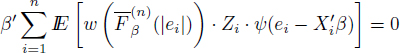
positive definite matrix, ![]() [Z1 · e] = 0 and define the estimator by means of the instrumental variables (IV) as the solution of the normal equations
[Z1 · e] = 0 and define the estimator by means of the instrumental variables (IV) as the solution of the normal equations
(An alternative way how to cope with the broken orthogonality condition is to utilize the orthogonal regression – sometimes called the total least squares, e.g. Paige and Strako 2002). There are several alternative ways to define the instrumental variables – see (Víšek 2017) and references given there – but all of them are practically equivalent to [4.15]; for the discussion which summarizes also geometric background of the instrumental variables, see again Víšek (2017). To prove the unbiasedness and consistency of classical instrumental variables, we do not need (nearly) any additional assumptions except of those which are given several lines above [4.15].
DEFINITION 4.2.– Let ![]() be a sequence of i.i.d. r.v.’s, such that
be a sequence of i.i.d. r.v.’s, such that ![]() Z1 = 0,
Z1 = 0, ![]() positive definite matrix,
positive definite matrix, ![]() [Z1 · e] = 0. The solution of the normal equation
[Z1 · e] = 0. The solution of the normal equation
will be called the estimator by means of the S-weighted instrumental variables (briefly, the S-weighted instrumental variables) and denoted by ![]() .
.
To be able to prove the consistency of ![]() , we will need some additional assumptions and an identification condition, similar to condition
, we will need some additional assumptions and an identification condition, similar to condition ![]() 3. We will start with an enlargement of notations.
3. We will start with an enlargement of notations.
Let for any β ∈ Rp and ![]() and
and ![]() be the d.f. of
be the d.f. of ![]() and e.d.f. of
and e.d.f. of ![]() respectively. Further, for any λ ∈ R+ and any a ∈ R put
respectively. Further, for any λ ∈ R+ and any a ∈ R put
CONDITION C4.– The instrumental variables ![]() are independent and identically distributed with distribution function FZ(z). Further, the joint distribution function FX,Z(x, z) is absolutely continuous with a density fX,Z(x, z) bounded by UZX < ∞. Further for any n ∈ N , we have
are independent and identically distributed with distribution function FZ(z). Further, the joint distribution function FX,Z(x, z) is absolutely continuous with a density fX,Z(x, z) bounded by UZX < ∞. Further for any n ∈ N , we have ![]() and the matrices
and the matrices ![]() as well as
as well as ![]() are positive definite. Moreover, there is q > 1 so that
are positive definite. Moreover, there is q > 1 so that ![]() Finally, there is a > 0, b ∈ (0, 1) and λ > 0 so that
Finally, there is a > 0, b ∈ (0, 1) and λ > 0 so that
for γλ,a and τλ given by [4.17].
LEMMA 4.2.– Let conditions ![]() 1 ,
1 , ![]() 2,
2, ![]() 4 be fulfilled and
4 be fulfilled and ![]() be a weakly consistent estimator of varFe(e) fulfilling the constraint [4.6]. Then for any ε > 0, there is ζ > 0 and δ > 0 such that
be a weakly consistent estimator of varFe(e) fulfilling the constraint [4.6]. Then for any ε > 0, there is ζ > 0 and δ > 0 such that
In other words, any sequence ![]() of the solutions of the sequence of normal equations [4.16]
of the solutions of the sequence of normal equations [4.16] ![]() is bounded in probability.
is bounded in probability.
The proof is formally nearly the same as the proof of lemma 1 in Vísek (2009). The allowance for the heteroscedasticity of disturbances requires some formally straightforward modifications. The fact that the modifications are relatively simple and straightforward is due to the fact that the complicated steps were made in (Víšek 2011b) but the background of proof is different from the proof in (Víšek 2009). The approximation of empirical d.f. is not by the underlying d.f. as the limit of the empirical d.f.’s but we employ the knowledge about convergence of the difference of the empirical d.f.’s and the arithmetic mean of the d.f.’s of individual disturbances (see lemma 4.1)
![]()
LEMMA 4.3.– Let conditions ![]() 1,
1, ![]() 2 and
2 and ![]() 4 be fulfilled and
4 be fulfilled and ![]() be a weakly consistent estimator of varFe(e) fulfilling the constraint [4.6]. Then for any ε > 0, δ ∈ (0, 1) and ζ > 0 there is nε,δ,ζ ∈
be a weakly consistent estimator of varFe(e) fulfilling the constraint [4.6]. Then for any ε > 0, δ ∈ (0, 1) and ζ > 0 there is nε,δ,ζ ∈ ![]() so that for any n > nε,δ,ζ we have
so that for any n > nε,δ,ζ we have
(for ai(β), see a line above [4.2] and for ![]() see [4.2] ).
see [4.2] ).
The proof has formally similar structure as the proof of lemma 2 in Vísek (2009). It is a bit more complicated because instead of employing a limiting distribution, we need to estimate differences of empirical d.f. of ai(β)’s from a sequence of the arithmetic means of underlying d.f.’s 
![]()
LEMMA 4.4.– Let conditions ![]() 1,
1, ![]() 2 and
2 and ![]() 3 hold and
3 hold and ![]() be a weakly consistent estimator of varFe(e) fulfilling the constraint [4.6]. Then for any positive ζ
be a weakly consistent estimator of varFe(e) fulfilling the constraint [4.6]. Then for any positive ζ
(for ![]() , see [4.10]) is uniformly in i ∈
, see [4.10]) is uniformly in i ∈ ![]() , uniformly continuous in β on
, uniformly continuous in β on ![]() = {β ∈ Rp : ∥β ∥ ≤ ζ}, i.e. for any ε > 0 there is δ > 0 so that for any pair of vectors β(1), β(2) ∈ Rp, ∥ β(1) − β(2)∥ < δ we have
= {β ∈ Rp : ∥β ∥ ≤ ζ}, i.e. for any ε > 0 there is δ > 0 so that for any pair of vectors β(1), β(2) ∈ Rp, ∥ β(1) − β(2)∥ < δ we have
The proof is a chain of approximations utilizing simple estimates of upper bounds of differences of the values of [4.19] for close pair of points in Rp.
![]()
Similarly as for the S-weighted estimator, we need for the S-weighted instrumenal variables the identification condition.
CONDITION ![]() 4.– For any n ∈
4.– For any n ∈ ![]() , the equation
, the equation
in the variable β ∈ Rp has a unique solution at β = β0.
THEOREM 4.2.– Let conditions ![]() 1,
1, ![]() 2,
2, ![]() 3 and
3 and ![]() 4 be fulfilled and
4 be fulfilled and ![]() be a weakly consistent estimator of varFe(e) fulfilling the constraint [4.6]. Then any sequence
be a weakly consistent estimator of varFe(e) fulfilling the constraint [4.6]. Then any sequence ![]() of the solutions of normal equations [4.16]
of the solutions of normal equations [4.16] ![]() is weakly consistent.
is weakly consistent.
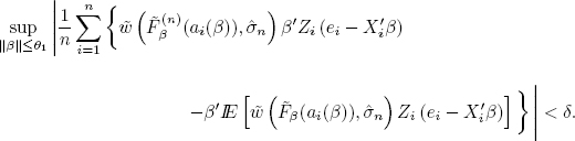
PROOF.– Without loss of generality assume that ![]() is scale and regression equivariant). To prove the consistency, we have to show that for any ε > 0 and δ > 0, there is nε,δ ∈
is scale and regression equivariant). To prove the consistency, we have to show that for any ε > 0 and δ > 0, there is nε,δ ∈ ![]() such that for all n > nε,δ
such that for all n > nε,δ
So fix ε1 > 0 and δ1 > 0. According to lemma 4.2, δ1 > 0 and θ1 > 0, so that for ε1 there is nδ1,ε1 ∈ ![]() ; for any n > nδ1,ε1
; for any n > nδ1,ε1
(denote the corresponding set by Bn). It means that for all n > nδ1,ε1, all solutions of the normal equations [4.16] ![]() are inside the ball B(0, θ1) with probability at least
are inside the ball B(0, θ1) with probability at least ![]() we have finished the proof. Generally, of course, we can have θ1 > δ.
we have finished the proof. Generally, of course, we can have θ1 > δ.
Then, using lemma 4.3 we may find for ε1 ![]() such nε1,δ,θ1 ∈
such nε1,δ,θ1 ∈ ![]() , nε1,δ,θ1 ≥ nδ1,ε1, so that for any n > nε1,δ,θ1, there is a set Cn (with P(Cn) > 1 −
, nε1,δ,θ1 ≥ nδ1,ε1, so that for any n > nε1,δ,θ1, there is a set Cn (with P(Cn) > 1 − ![]() such that for any ω ∈ Cn
such that for any ω ∈ Cn
But it means that
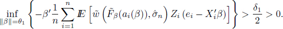
Further consider the compact set C = {β ∈ Rp : δ1 ≤ ∥β∥≤ θ1} and find
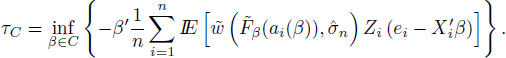
Then there is a ![]() such that
such that
On the other hand, due to compactness of C, there is a β∗ and a subsequence ![]() such that
such that
and due to the uniform continuity (uniform in i ∈ ![]() as well as in β ∈ C) of
as well as in β ∈ C) of ![]() (see lemma 4.4), we have
(see lemma 4.4), we have
Employing once again the uniform continuity (uniform in i ∈ ![]() and β ∈ C) of
and β ∈ C) of ![]() together with condition
together with condition ![]() 4 and [4.22] we find that τC > 0, otherwise there has to be a solution of [4.20] inside the compact C, which does not contain β = 0.
4 and [4.22] we find that τC > 0, otherwise there has to be a solution of [4.20] inside the compact C, which does not contain β = 0.
Now, using lemma 4.3 once again we may find for ε1, δ1, θ1 and τC nε1,δ1,θ1,τC ∈ ![]() , nε1,δ1,θ1,τC ≥ nε1,δ,θ1, so that for any n > nε1,δ1,θ1,τC there is a set Dn (with
, nε1,δ1,θ1,τC ≥ nε1,δ,θ1, so that for any n > nε1,δ1,θ1,τC there is a set Dn (with ![]() such that for any ω ∈ Dn
such that for any ω ∈ Dn
But [4.23] and [4.25] imply that for any n > nε1, δ1, θ1, τC and any ω ∈ Bn ∩ Dn
we have
Of course, P (Bn ∩ Dn) > 1 − ε1. But it means that all solutions of normal equations [4.16] are inside the ball of radius δ1 with probability at least 1 − ε1, i.e. in other words, ![]() is weakly consistent.
is weakly consistent.
![]()
4.5. Patterns of results of simulations
In the simulations, we compared S-weighted instrumental variables with classical instrumental variables (which is not robust) and with three other robust versions of instrumental variables, namely instrumental weighted variables (see Víšek 2017), S-instrumental variables and W-instrumental variables (see Cohen-Freue et al. 2013, Desborges and Verardi 2012; unfortunately the description of these estimators would require rather large space, so we only refer to original papers). The best results from these three alternative estimators were achieved by the S-instrumental variables and instrumental weighted variables, and we decided to report, in Tables 4.1, 4.2 and 4.3, S-instrumental variables (the lack of space has not allowed us to present more).
4.5.1. Generating the data
The data were generated for i = 1, 2, .., n, t = 1, 2, …, T according to the model
with Xit+1 = 0.9 · Xit + 0.1 · vit + 0.5 · eit where the initial value ![]() the innovations
the innovations ![]() and the disturbances
and the disturbances ![]() were i.id. four dimensional normal vectors with the zero means and the unit covariance matrix. Sequence
were i.id. four dimensional normal vectors with the zero means and the unit covariance matrix. Sequence ![]() is i.i.d., distributed uniformly over [0.5, 5.5]. In the role of the objective function, we have employed Tukey’s ρ given for some c > 0 as
is i.i.d., distributed uniformly over [0.5, 5.5]. In the role of the objective function, we have employed Tukey’s ρ given for some c > 0 as
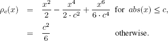
For 0 < h < g < 1, the weight function w(r) : [0, 1] → [0, 1] is equal to 1 for 0 ≤ r ≤ h, it is equal to 0 for g ≤ r ≤ 1 and it decreases from 1 to 0 for h ≤ r ≤ g, i.e. putting c = g − h and y = g − r, we compute
i.e. between h and g the weight function borrowed the shape from Tukey’s ρ.
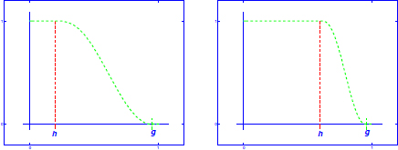
Figure 4.1. The examples of possible shapes of weight function. For a color version of this figure, see www.iste.co.uk/skiadas/data1.zip
The data were contaminated so that we selected randomly one block (i.e. one ![]() and either the bad leverage points were created as X(new) = 5 . X(original) and Y (wrong) = −Y (correct) or the outliers were created as Y (wrong) = −3 · Y (correct). The data contained the same number of good leverage points X(new) = 20 · X(original) (with the response Y calculated correctly) as bad leverage points.
and either the bad leverage points were created as X(new) = 5 . X(original) and Y (wrong) = −Y (correct) or the outliers were created as Y (wrong) = −3 · Y (correct). The data contained the same number of good leverage points X(new) = 20 · X(original) (with the response Y calculated correctly) as bad leverage points.
4.5.2. Reporting the results
We have generated 500 sets, each containing n · T observations (it is specified in heads of tables) and then we calculated the estimates
where the abbreviations IV, SIV and SWIV at the position of “index” indicate the method employed for the computation, namely IV – for the instrumental variables, SIV – for S-instrumental variables estimator and finally SWIV – for S-weighted instrumental variables estimator. The empirical means and the empirical mean squared errors (MSE) of estimates of coefficients (over these 500 repetitions) were computed, i.e. we report values (for j = 1, 2, 3, 4 and 5)
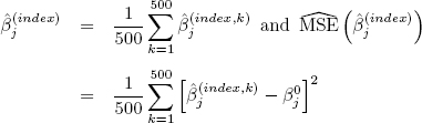
where β0 = [1, −2, 3, −4, 5]′ and the index have the same role as above. The results are given in tables in the form as follows: the first cell of each row indicates the method, e.g. ![]() , the next five cells contain then just
, the next five cells contain then just ![]() , for the first, the second up to the fifth coordinate.
, for the first, the second up to the fifth coordinate.
As discussed previously, it is believed that the leverage points are more complicated problem than outliers. Table 4.3 offers results indicating that the “classical” estimators as the LMS, the LTS or the S-estimator can exhibit a problem when data contain a group of good leverage points (far away from the main bulk of data) and some outliers (not very far from the bulk of data). As the mean squared errors of the S-estimates below indicate that the S-estimator have used the information in data less efficiently than S-weighted estimator (see [4.5]). (Due to the lack of space we present only the results for the S-estimator – which were the best among the “classical” estimators (LMS, LTS, LWS and S-estimator). The reason for large MSE of the S-estimates is the depression of the information brought by good leverage points. It happened due to the implicit estimation of variance of disturbances.
Table 4.1. The contamination by leverage points on the level of 1%, n = 100. The values of variance of the disturbances randomly selected from [0.5, 5.5]
| T = 1, n. T = 100, h = 0.98, g = 0.99 | |||||
| 0.970 (0.372) | −1.924 (0.375) | 2.835 (0.419) | −3.781 (0.429) | 4.706 (0.479) | |
| 0.993 (0.105) | −1.986 (0.133) | 2.979 (0.141) | −4.021 (0.151) | 4.987 (0.142) | |
| 0.992 (0.106) | −1.990 (0.105) | 3.002 (0.122) | −4.000 (0.120) | 4.992 (0.105) | |
| T = 2, n. T = 200, h = 0.98, g = 0.99 | |||||
| 0.966 (0.319) | −1.873 (0.404) | 2.814 (0.378) | −3.808 (0.369) | 4.690 (0.605) | |
| 0.993 (0.056) | −2.004 (0.082) | 3.007 (0.077) | −4.017 (0.071) | 4.984 (0.084) | |
| 0.993 (0.059) | −1.997 (0.069) | 3.009 (0.061) | −4.002 (0.058) | 4.992 (0.068) | |
| T = 3, n. T = 300, h = 0.98, g = 0.99 | |||||
| 0.982 (0.259) | −1.879 (0.323) | 2.795 (0.363) | −3.734 (0.453) | 4.678 (0.532) | |
| 1.002 (0.037) | −2.017 (0.050) | 2.995 (0.057) | −4.009 (0.057) | 4.989 (0.058) | |
| 0.999 (0.039) | −2.006 (0.041) | 2.990 (0.050) | −3.989 (0.046) | 4.995 (0.047) | |
| T = 4, n. T = 400, h = 0.98, g = 0.99 | |||||
| 0.961 (0.213) | −1.887 (0.280) | 2.863 (0.290) | −3.764 (0.403) | 4.743 (0.380) | |
| 0.995 (0.027) | −2.022 (0.046) | 2.986 (0.052) | −4.017 (0.047) | 4.981 (0.049) | |
| 0.994 (0.029) | −2.013 (0.038) | 2.992 (0.042) | −4.014 (0.038) | 4.986 (0.036) | |
| T = 5, n. T = 500, h = 0.98, g = 0.99 | |||||
| 0.964 (0.194) | −1.859 (0.360) | 2.806 (0.393) | −3.781 (0.334) | 4.717 (0.407) | |
| 1.003 (0.025) | −2.007 (0.042) | 2.995 (0.041) | −4.006 (0.042) | 4.997 (0.045) | |
| 1.002 (0.025) | −2.006 (0.032) | 2.991 (0.033) | −4.000 (0.033) | 5.004 (0.036) | |
Table 4.2. The contamination by leverage points on the level of 5%,n = 100. The values of variance of the disturbances randomly selected from [0.5, 5.5].
| T = 5, n. T = 100, h = 0.940, g = 0.948 | |||||
| 0.879 (4.420) | −1.505 (6.863) | 2.335 (6.609) | −3.096 (7.212) | 3.730 (7.995) | |
| 0.992 (0.662) | −1.953 (0.946) | 2.824 (1.243) | −3.920 (1.017) | 4.672 (2.158) | |
| 0.982 (0.178) | −1.982 (0.336) | 2.981 (0.349) | −4.018 (0.296) | 4.954 (0.362) | |
| T = 10, n. T = 200, h = 0.940, g = 0.948 | |||||
| 0.862 (2.967) | −1.604 (3.871) | 2.548 (3.839) | −3.227 (4.665) | 4.011 (5.258) | |
| 0.990 (0.138) | −2.001 (0.349) | 2.971 (0.350) | −3.997 (0.273) | 4.933 (0.389) | |
| 0.990 (0.082) | −1.993 (0.140) | 3.010 (0.138) | −3.992 (0.133) | 5.010 (0.154) | |
| T = 15, n. T = 300, h = 0.940, g = 0.948 | |||||
| 0.755 (1.912) | −1.479 (3.644) | 2.431 (3.242) | −3.324 (4.295) | 3.980 (4.988) | |
| 0.984 (0.053) | −2.020 (0.219) | 2.934 (0.233) | −4.020 (0.236) | 4.897 (0.218) | |
| 0.985 (0.048) | −2.008 (0.107) | 2.995 (0.121) | −4.017 (0.104) | 4.975 (0.112) | |
| T = 20, n. T = 400, h = 0.940, g = 0.948 | |||||
| 0.774 (1.463) | −1.562 (2.618) | 2.577 (2.490) | −3.374 (2.845) | 4.220 (2.826) | |
| 0.992 (0.036) | −1.988 (0.199) | 2.934 (0.191) | −3.974 (0.176) | 4.948 (0.169) | |
| 0.994 (0.033) | −1.986 (0.076) | 3.006 (0.078) | −3.981 (0.077) | 5.017 (0.072) | |
| T = 25, n. T = 500, h = 0.940, g = 0.948 | |||||
| 0.794 (1.074) | −1.629 (1.644) | 2.494 (1.923) | −3.551 (1.722) | 4.314 (2.187) | |
| 0.990 (0.034) | −1.983 (0.168) | 2.930 (0.172) | −3.991 (0.151) | 4.944 (0.209) | |
| 0.993 (0.028) | −1.985 (0.062) | 2.984 (0.069) | −3.995 (0.060) | 4.996 (0.065) | |
Table 4.3. Contamination by outliers: For randomly selected observations, we put ![]() and data contained also good leverage points
and data contained also good leverage points ![]() and responses Yi’s were computed correctly
and responses Yi’s were computed correctly
| Number of observations in each data set = 500 | |||||
| Contamination level = 1%, h = 0.973, g = 0.989 | |||||
| 1.010 (0.024) | 2.003 (0.031) | −3.021 (0.032) | 3.975 (0.035) | −4.974 (0.023) | |
| 1.002 (0.022) | 2.001 (0.013) | −3.012 (0.011) | 3.986 (0.010) | −4.990 (0.011) | |
| Contamination level = 2%, h = 0.963, g = 0.978 | |||||
| 0.993 (0.027) | 2.014 (0.032) | −2.973 (0.027) | 3.985 (0.028) | −4.996 (0.023) | |
| 0.992 (0.030) | 2.008 (0.005) | −3.000 (0.004) | 4.000 (0.005) | −5.003 (0.004) | |
| Contamination level = 5%, h = 0.921, g = 0.942 | |||||
| 0.985 (0.028) | 1.948 (0.040) | −2.967 (0.034) | 3.919 (0.038) | −4.955 (0.030) | |
| 1.014 (0.027) | 2.002 (0.002) | −3.006 (0.002) | 3.998 (0.002) | −5.003 (0.001) | |
Generally, the implicit estimation of variance of the disturbances (e.g. by LMS, LTS or LWS) is the significant advantage (from the computational point of view) because the estimators do not need any studentization – contrary to M-estimators – see (Bickel 1975). Sometimes, it can betray us.
4.6. Acknowledgment
This study was performed with the support of the Czech Science Foundation project P402/12/G097’DYME – Dynamic Models in Economics.
4.7. References
Bickel, P.J. (1975). One-step Huber estimates in the linear model. J. Amer. Statist. Assoc. 70, 428–433.
Boček, P., Lachout, P. (1993). Linear programming approach to LMS-estimation. Memorial volume of Comput. Statist. & Data Analysis, 19(1995), 129–134.
Breiman, L. (1968). Probability. Addison-Wesley Publishing Company, London.
Campbell, N.A., Lopuhaa, H.P., Rousseeuw, P.J. (1998). On calculation of a robust S-estimator if a covariance matrix. Statistics in medcine, 17, 2685–2695.
Carroll, R.J., Stefanski, L.A. (1994). Measurement error, instrumental variables and correction for attenuation with applications to meta-analyses. Statistics in Medicine, 13, 1265–1282.
Číek, P., Víšek, J.Á. (2000). The least trimmed squares. User Guide of Explore, Humboldt University, Berlin.
Cohen-Freue, G.V., Ortiz-Molina, H., Zamar, R.H. (2013). Natural robustification of the ordinary instrumental variables estimator. Biometrics, 69, 641–650.
Desborges, R., Verardi, V. (2012). A robust instrumental-variable estimator. The Stata Journal, 12, 169–181.
Hájek, J., Šidák, Z. (1967). Theory of Rank Test. Academic Press, New York.
Hampel, F.R., Ronchetti, E.M., Rousseeuw, P.J., Stahel, W.A. (1986). Robust Statistics – The Approach Based on Influence Functions. John Wiley & Sons, New York.
Heckman, J., Urza, S., Vytlacil, E.J. (2006). Understanding instrumental variables in models with essential heteroscedasticity. Working paper 12574, National Bureau of Economic Research, 2006.
Hawkins, D.M. (1994). The feasible solution algorithm for least trimmed squares regression. Computational Statistics and Data Analysis 17, 185–196.
Hawkins, D.M., Olive, D.J. (1999). Improved feasible solution algorithms for breakdown estimation. Computational Statistics & Data Analysis 30, 1–12.
Hettmansperger, T.P., Sheather, S.J. (1992). A cautionary note on the method of least median squares. The American Statistician 46, 79–83.
Koenker, R., Bassett, G. (1978). Regression quantiles. Econometrica, 46, 33–50.
Maronna, R.A., Yohai, V. (1981). Asymptotic behavior of general M-estimates for regression and scale with random carriers. Z. Wahrscheinlichkeitstheorie verw, Gebiete 58, 7–20.
Paige, C.C., Strako, Z. (2002). Scaled total least squares fundamentals. Numerische Mathematik, 91, 117–146.
Rousseeuw, P.J. (1983). Multivariate estimation with high breakdown point. In Mathematical Statistics and Applications B, Grossmann, W., Pflug, G., Vincze, I., Wertz, W. (eds), Reidel, Dordrecht, 283–297.
Rousseeuw, P.J. (1984). Least median of square regression. Journal of Amer. Statist. Association, 79, 871–880.
Rousseeuw, P.J., Yohai, V. (1984). Robust regression by means of S-estimators. In Robust and Nonlinear Time Series Analysis: Lecture Notes in Statistics No. 26, Franke, J., Härdle, W.H, Martin, R.D. (eds), Springer Verlag, New York, 256–272.
Siegel, A.F. (1982). Robust regression using repeated medians. Biometrica, 69, 242–244.
Víšek, J.Á. (1990). Empirical study of estimators of coefficients of linear regression model. Technical report of Institute of Information Theory and Automation, Czechoslovak Academy of Sciences, 1699.
Víšek, J.Á. (1998). Robust instruments. In Robust’98, Antoch, J., Dohnal, G. (eds), Union of Czech Mathematicians and Physicists, Matfyzpress, Prague, 195–224.
Víšek, J.Á. (2000). Regression with high breakdown point. In Robust 2000, Antoch, J., Dohnal, G. (eds), The Union of the Czech Mathematicians and Physicists and the Czech Statistical Society 2001, Matfyzpress, Prague, 324–356.
Víšek, J.Á. (2002). The least weighted squares II. Consistency and asymptotic normality. Bulletin of the Czech Econometric Society, 9, 1–28.
Víšek, J.Á. (2004). Robustifying instrumental variables. In Proceedings of COMPSTAT’ 2004, Antoch, J. (ed.), Physica-Verlag/Springer, 1947–1954.
Víšek, J.Á. (2006). The least trimmed squares. Part I – Consistency. Part II – √n-consistency. Part III – Asymptotic normality and Bahadur representation. Kybernetika, 42, 1–36, 181–202, 203–224.
Víšek, J.Á. (2006). Instrumental weighted variables. Austrian Journal of Statistics, 35, 379–387.
Víšek, J.Á. (2006). Instrumental weighted variables – algorithm. In Proceedings of COMPSTAT 2006, Rizzi, A., Vichi, M. (eds), Physica-Verlag, Springer Company, Heidelberg, 777–786.
Víšek, J.Á. (2009). Consistency of the instrumental weighted variables. Annals of the Institute of Statistical Mathematics, 61, 543–578.
Víšek, J.Á. (2011). Empirical distribution function under heteroscedasticity. Statistics, 45, 497–508.
Víšek, J.Á. (2011). Consistency of the least weighted squares under heteroscedasticity. Kybernetika, 47, 179–206.
Víšek, J.Á. (2015). S-weighted estimators. In Proceedings of the 16th Conference on the Applied Stochastic Models, Data Analysis and Demographics, Skiadas, C.H. (ed.), 1031-1042 or Stochastic and Data Analysis Methods and Applications in Statistics and Demography, Bozeman, J.R., Oliveira, T., Skiadas, C.H. (eds), 437–448.
Víšek, J.Á. (2016). Representation of SW-estimators. In Proceedings of the 4th Stochastic Modeling Techniques and Data Analysis International Conference with Demographics Workshop, SMTDA 2016, Skiadas, C.H. (ed.), 425–438.
Víšek, J.Á. (2017). Instrumental weighted variables under heteroscedasticity. Part I. Consistency. Part II. Numerical study. Kybernetika, 53(2017), 1-25, 26–58.
Wagenvoort, R., Waldmann, R. (2002). On B-robust instrumental variable estimation of the linear model with panel data. Journal of Econometrics, 106, 297–324.
Chapter written by Jan Ámos VÍŠEK.