13
Frost Prediction in Apple Orchards Based upon Time Series Models
The scope of this work was to evaluate the autoregressive integrated moving average (ARIMA) model as a frost forecast model for South Tyrol in Italy using weather data of the past 20 years that were recorded by 150 weather stations located in this region. Accurate frost forecasting should provide growers with the opportunity to prepare for frost events in order to avoid frost damage. The radiation frost in South Tyrol occurs during the so-called frost period, i.e. in the months of March, April and May during calm nights between sunset and sunrise. In case of a frost event, the farmers should immediately switch on water sprinklers. The ice cover that builds on the trees protects the buds and blossoms from damage. Based on the analysis of time series data, the linear regression (LR) and ARIMA models were compared and evaluated. The best result was achieved by the ARIMA model, with the optimal value of 1.0 for recall in case of forecast of 95% confidence intervals. This means that all frost cases could be correctly predicted. Despite the encouraging results for recall, the rate of false positives with a sensitivity of 21% is too high, such that further investigations are desirable (e.g. testing VARIMA models, which are a multivariate extension of ARIMA models). The graphical illustration of the 95% confidence intervals of the ARIMA model forecast and the linear models forecast should be helpful in frost prediction and could be integrated in the electronic monitoring system that permits forecasting of frost weather phenomena.
13.1. Introduction
Accurate frost forecasting should provide growers in South Tyrol with the opportunity to prepare for frost events in order to avoid frost damage. The higher the level of forecast accuracy, the lower the risk of frost damage. Damage to apple orchards brought by freezing night temperatures can cause high crop yield losses to the growers. The critical periods for frost damage in apple orchards are the months of spring: March, April and May. The radiation frost occurs during clear nights with little or no wind after sunset and lasts until after sunrise.
Overplant conventional sprinklers are widely used in South Tyrol as effective frost protection method for apple orchards. The ice cover prevents the temperature of the protected plant from falling below the freezing point. Sprinkling must start with the onset of the critical temperature and be maintained until the temperature rises above 0° C. This work describes frost prediction in apple orchards based upon a non-seasonal autoregressive integrated moving average (ARIMA) model and three different linear (LR) models.
The general autoregressive moving average (ARMA) model was described first in 1951 by Peter Whittle in his thesis “Hypothesis testing in time series analysis”. The ARIMA model is a generalization of the ARMA model. Nowadays, it is widely used in time series analysis. However, there exists only little literature about frost forecasting with ARIMA.
In Castellanos et al. (2009), the authors used the ARIMA model to forecast the minimum monthly absolute temperature and the average monthly minimum temperature following the Box and Jenkins methodology.
Another interesting research project about frost forecasting of minimum temperature in the Alpine area is described by Eccel et al. (2008). In this work, a simple LR model, a random forest (RF) model and a neural network (NN) model were compared and evaluated. The results achieved by RF were slightly superior to those of other methods. The LR model for frost forecasting was introduced and implemented by Snyder et al. (2005).
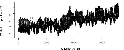
13.2. Weather database
The weather database holds data from about 150 weather stations, which have been operating since 1993. The weather stations are distributed in apple orchards at an elevation between 200 and 1,100 m.a.s.l.
Currently, the database continues to receive data every 5 min via radio waves or GPRS. The measurements include atmospheric conditions, air and soil temperature, relative air humidity, soil humidity at a depth of 10, 30 and 50 cm, wind speed and direction, precipitation amounts and the relative humidity at leaf surfaces. Moreover, the database contains information of the geographic coordinates of each station (latitude, longitude and altitude).
The historical climate patterns of the past 20 years stored in the weather database can serve as indicator of the climate for future time points. Based on the measurements of the past years, we calculated the forecast of frost weather phenomena and compared the prediction against the observed temperature in order to evaluate the results.
Table 13.1. Variables that were recorded by the weather stations
| Measurement | Unit |
| Wet bulb temp (60 cm) | °C |
| Dry bulb temp (60 cm) | °C |
| Rel. air humidity | % |
| Air temp (2 m) | °C |
| Wind speed | m/sec |
| Wind direction | N/S/E/W |
| Leaf surface humidity | % |
| Precipitation | mm |
| Irrigation | ON/OFF |
| Irrigation | mm |
| Soil temp (–25 cm) | °C |
| Min interval air temp (2 m) | °C |
| Max interval air temp (2 m) | °C |
| Min interval rel. air humidity | % |
| Max interval rel. air humidity | % |
| Max interval wind speed | m/sec |
| Soil humidity (–10 cm) | % |
| Soil humidity (–30 cm) | % |
| Soil humidity (–50 cm) | % |
13.3. ARIMA forecast model
ARIMA models are a widely used approach to time series forecasting based on autocorrelations in the data.
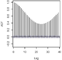
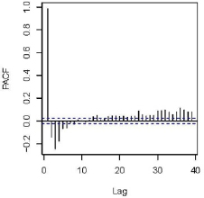
13.3.1. Stationarity and differencing
ARIMA models as described by Hyndman and Athanasopoulos (2012) require that the time series to which they are applied be stationary. A stationary time series is one whose properties like the mean, variance and autocorrelation do not depend on the time point at which the series is observed. A stationary time series has no predictable pattern in the long term. The time plots show a horizontal pattern with constant variance. A non-stationary time series can be transformed into a stationary one by computing the differences between consecutive observations. This transformation is known as differencing. The first-order differenced series can be written as
If the result of the first-order differencing is still a non-stationary time series, second-order differencing can be applied to obtain a stationary time series (Hyndman and Athanasopoulos 2012):
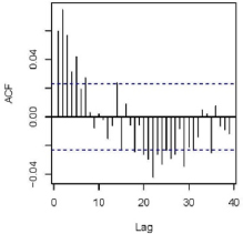
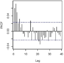
One approach to identify non-stationarity is an autocorrelation function (ACF) plot. The ACF plot shows the autocorrelations, which measure the relationship between yt and yt−k for k (k = 1, 2, 3….) lags. In case of non-stationarity, the ACF will slowly decrease.
Furthermore, widely used tests are the Kwiatkowski–Phillips–Schmidt–Shin (KPSS) test and the augmented Dickey–Fuller (ADF) test.
13.3.2. Non-seasonal ARIMA models
The non-seasonal ARIMA model described by Hyndman and Athanasopoulos (2012) is a combination of an AR(p) model, differencing and an MA(q) model, and can be written as:
where:
- – y′t is the differenced series;
- – et is white noise;
- – c is a constant;
- – p and q are the order of the AR and the MA model, respectively.
A non-seasonal ARIMA model is written as
where:
- – p is the order of the autoregressive part AR(p);
- – d is the degree of first differencing involved;
- – q stands for order of the moving average part MA(q).
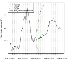
Figure 13.7. ARIMA(4,1,4) forecast from 22:00 until sunrise. The observed temperature is shown as full line
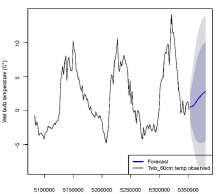
Figure 13.8. ARIMA(4,1,4) forecast shown with the temperature of the previous three days
In Figure 13.7, a forecast plot for ARIMA(4,1,4) built on the wet bulb temperature time series is shown (March 4, 2006) for the station 14 in Terlano as a green dashed line together with the observed data and the confidence intervals. In this example, the point forecast suits well the real data. Figure 13.8 shows the forecast plot (blue line) with blue shadowed confidence intervals together with the observed time series data of the previous 3 days.
13.4. Model building
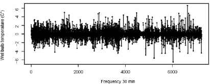
As preliminary step for the analysis, we tested ARIMA models for the wet bulb and dry bulb temperature time series. We ran numerous trials in order to optimize the length of time series to be included in the model and the time frequencies. The results were best when the frequency was observed at 30 min and the length was approximately equal to the length of the frost period. We also compared the results of the manually created ARIMA models following the steps of the procedure described by Hyndman and Athanasopoulos (2012) with those created by the automatic ARIMA function auto.arima() from the R package “forecast” for “Forecasting Functions for Time Series and Linear Models”. Altogether, the results obtained manually and automatically were quite comparable.
For the calculation of the sunrise and sunset time, we used the geographic coordinates of the station from the database.
13.4.1. ARIMA and LR models
The scope of the first analysis was to compare automatically modeled ARIMA [13.4] for the dry bulb temperature time series and three LR forecast models, which are variations of the model described by Snyder et al. (2005):
where:
- – TdbSunrise is the dry bulb temperature at 60 cm above ground at sunrise;
- – TdbSunset is the dry bulb temperature at 60 cm above ground at sunset;
- – TdpSunset stands for the dew point temperature at sunset;
- – TwbSunset is the wet bulb temperature at 60 cm above ground at sunset;
- – RHSunset is relative humidity at sunset.
For the test, 100 forecasts for each model were calculated and tested on a randomly chosen data set. The point forecast, lower bound of the 80% and the 95% confidence interval were calculated.
13.4.2. Binary classification of the frost data
The following test conditions were defined:
- – frost: positive condition, when the predicted variable dry bulb temperature at 60 cm above ground falls below 0°C at sunrise;
- – no frost: negative condition, when the predicted variable dry bulb temperature at 60 cm above ground does not fall below 0°C at sunrise.
13.4.3. Training and test set
The data set for the forecast was selected in the following manner:
- 1) choose randomly one station from all stations;
- 2) choose randomly 1 year from the range of years;
- 3) choose randomly 1 day for the forecast from the relevant frost period (from March until May).
We randomly selected 47 frost cases and 53 days without frost, altogether 100 days. As a training set, a 30-day time period before the previously randomly selected day of the forecast was chosen. As a test set served the day of the forecast itself. Next, the following two-step procedure was conducted:
- 1) calculate the ARIMA non-seasonal model on the training set;
- 2) test the model on the test set.
13.5. Evaluation
In order to assess the quality of a forecast, we considered the following quantities: accuracy, recall and specificity. Accuracy is defined as the ratio of all correctly recognized cases to the total number of test cases. The recall is defined as ratio of true positives to all frost cases. The specificity is the ratio of true negatives to all no frost cases.
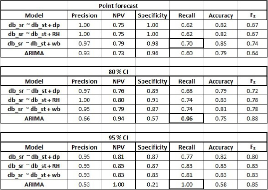
On the basis of the recall value for the point forecast, the LR model 3 with recall value equal to 70% could be identified as the best model. The two other LR models and the ARIMA model reached a recall value of about 60%. The specificity values for all models were between 96% and 100%. The accuracy for the point forecast was between 79% (ARIMA) and 85% (LR model 3). The test results for the 80% and 95% confidence intervals for the LR models were quite similar. Their recall values ranged from 68% to 83%, the specificity from 85% to 91% and the accuracy from 79% and 85%. The model 2 was the best in this group for both confidence intervals. For the test level of the 80% and 95% confidence interval lower bounds, the best model was ARIMA, which reached higher values for recall than the LR models. In case of the 95% CI lower bound, the optimal value of 1.0 for the recall was achieved. Unfortunately, the payoff of the good results for recall was a low value for specificity of 20% only, which resulted in a low accuracy of 58%.
Table 13.2. Evaluation results of ARIMA and linear regression models
13.6. ARIMA model selection
The scope of the second analysis was to study which ARIMA model parameters were selected for the forecast by the automatic model building function auto.arima() from the R package “forecast”. The forecast was made for 500 selected days. We chose randomly one station from the range of all stations, 1 year, 1 day from the frost period and calculated the model for the previous 30 days before the randomly selected day.
The results of the trial showed that there was a wide range of possible model parameter sets. The distribution of p and q values is shown in Figures 13.9 and 13.10, respectively. At the same time, it is notable that the p and q values are correlated. The higher is the p, the higher the q value. The correlation between p and q is shown in Figure 13.11. On the other hand, the p and q values are not correlated when d = 0, which confirmed the test for association between paired samples using Pearson’s product moment correlation coefficient. The P-value for the statistical significance was above the conventional threshold of 0.05, so the correlation is not statistically significant.
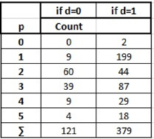
Figure 13.9. Count of p
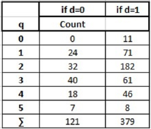
Figure 13.10. Count of q
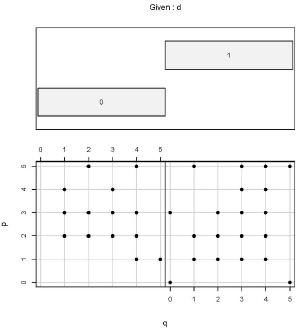
Figure 13.11. Conditional plot of p versus q at given d
13.7. Conclusions
This work described frost prediction in apple orchards based upon time series models: a non-seasonal ARIMA model and three different LR models. The model should help in the design of an electronic monitoring system that permits forecasting of frost weather phenomena. Based on analysis of time series data and numerous trials, the proposed models could be compared and evaluated. The following observations regarding temperature forecast for up to 12 h after sunset were made:
- – for the test level of the lower bound of the 80% and 95% confidence intervals, the ARIMA model reached higher values for recall (the ratio of correctly recognized frost cases to all frost cases) than the LR models. In case of ARIMA models and the lower bound of the 95% CI, the optimal value of 1.0 for the recall was achieved, which means that all frost cases could be correctly forecast;
- – unfortunately, the payoff of the good results for recall is the low value for the specificity of only 20%. This means risk of frequent false alarms.
Despite the high risk of false alarms, the ARIMA model offers encouraging results worth further investigations. LR models can be further improved as well. Here is a list of several complementary analysis steps, which could be tried out toward more accurate forecasting:
- – vector ARIMA models (VARIMA), a multivariate extension of ARIMA models, should be tested. The vector of predictors variable in LR models could be extended by wind speed and soil temperature, which would likely lead to more precise forecast;
- – the length of the training data can be still optimized in order to find the optimal fit;
- – the orders p and q of the ARIMA model should be studied in order to find out potential correlations with temperature. This would allow to exclude some of the models;
- – a similarity study of the forecast coming from different stations should be made. Such similarity information could turn out to be helpful in the ARIMA model selection.
13.8. Acknowledgments
The authors would like to thank Professor Johann Gamper of the Free University of Bozen-Bolzano, Faculty of Computer Science, who supported this research project.
13.9. References
Beratungsring. (2012). Leitfaden 2012.
Bootsma, A., Murray, D. (1985). Freeze Protection Methods for Crops. Factsheet. Ministry of Agriculture, Food and Rural Affairs, Guelph, ON.
Bowermann, B.L., O’Connell, R.T., Koehler, A.B. Forecasting, Time Series, and Regression. Thomson, Brooks/Cole, Pacific Grove, CA.
Castellanos, M.T., Tarquis, A.M., Morató, M.C. and Saa, A. (2009). Forecast of frost days based on monthly temperatures. Spanish Journal of Agricultural Research, 7(3), 513–524.
Eccel, E., Ghielmi, L., Granitto, P., Barbiero, R., Grazzini, F., Cesari, D. (2008). Techniche di post-elaborazione di previsione di temperatura minima a confronto per un’ area alpina. Italian Journal of Agrometeorology 3, 38–44.
Hyndman, R.J., Athanasopoulos, G. (2012). Forecasting: Principles and Practice. OTexts, Melbourne.
Oberhofer, H. (1969). Erfahrungen aus den Spätfrösten 1969. Obstbau Weinbau Mitteilungen des Südtiroler Beratungsringes.
Oberhofer, H. (1986). Eine Frostnacht – eine Lehre? Obstbau Weinbau Mitteilungen des Südtiroler Beratungsringes.
Snyder, R.L., de Melo-Abreu, J.P., Matulich, S. (2005). Frost Protection: Fundamentals, Practice, and Economics, volume 1. FAO, Rome.
Waldner, W. (1993). Was bewirken die Spätfröste Ende März? Obstbau Weinbau Mitteilungen des Südtiroler Beratungsringes.
Chapter written by Monika A. TOMKOWICZ and Armin O. SCHMITT.