
]>
16
An Application of Data Mining Methods to the Analysis of Bank Customer Profitability and Buying Behavior
In this chapter, we use a database from a Portuguese bank, with data related to the behavior of customers, to analyze churn, profitability and next-product-to-buy (NPTB). The database includes data from more than 94,000 customers, and includes all transactions and balances of bank products from those customers for the year 2015. We describe the main difficulties found concerning the database, as well as the initial filtering and data processing necessary for the analysis. We discuss the definition of churn criteria and the results obtained by the application of several techniques for churn prediction and for the short-term forecast of future profitability. Finally, we present a model for predicting the next product that will be bought by a client. The models show some ability to predict churn, but the fact that the data concerns just a year clearly hampers their performance. In the case of the forecast of future profitability, the results are also hampered by the short timeframe of the data. The models for the next product to buy show a very encouraging performance, being able to achieve a good detection ability for some of the main products of the bank.
16.1. Introduction
The huge amounts of data that banks currently possess about their customers allow them to make better decisions concerning the efforts to obtain new customers and the types of marketing campaigns they undertake. Better decisions are beneficial to the bank, since they may lead to increased profits, but they may also be beneficial to customers, who can now be targeted just by campaigns concerning products that may interest them.
One important piece of information that can be estimated from data in bank databases is the customer lifetime value (CLV). CLV can be understood as the total value that a customer produces during his/her lifetime (EsmaeiliGookeh and Tarokh 2013). There are many models for quantifying this value (see, for instance, Singh and Jain 2010 for a review of the most prominent models). Some existing models are based on the recency, frequency, monetary (RFM) framework (Fader et al. 2005) and Pareto/NBD (Schmittlein et al. 1987; Schmittlein and Peterson 1994) or related models (Fader et al. 2005, 2010). As pointed out by Blattberg et al. (2009), due to the uncertainty in future customer behavior, as well as in the behavior of the firm’s competitors and of the firm itself, CLV is indeed a random variable and methodologies should try to compute an expected CLV.
CLV prediction in the retail banking sector is especially difficult for a number of reasons, including product diversity (which can jeopardize the use of RFM-based approaches; Ekinci et al. 2014), the existence of both contractual and non-contractual clients (meaning that some clients are free to leave as soon as they want, while others have long-term contracts) and even the difficulty in identifying lost customers. Despite these difficulties, several authors have addressed the estimation of CLV in retail banks. Glady et al. (2009) use a modified Pareto/NBD approach to estimate CLV in the retail banking sector. The authors show that the dependence between the number of transactions and their profitability may be used to increase the accuracy in CLV prediction. Haenlein et al. (2007) present a model with four different groups of profitability drivers based on a classification and regression tree. Clients are clustered into different groups, and a transition matrix is used to consider movements between clusters. A CLV model based on RFM and Markov chains is proposed in Mzoughia and Limam (2015). Calculating the churn probability for a given client or cluster of clients may support the estimation of CLV. Ali and Arıtürk (2014) present a dynamic churn prediction framework that uses binary classifiers. Customer churn prediction is also tackled by He et al. (2014) by applying support vector machines.
Another important issue in retail banking is identifying the products that a customer is most likely to buy in order to enhance the effectiveness of cross-selling strategies or marketing campaigns. This may be addressed by NPTB models, which attempt to predict “which product (or products) a customer would be most likely to buy next, given what we know so far about the customer” (Knott et al. 2002).
Examples of works analyzing NTBD models and cross-selling strategies in banking can be found, for example, in Knott et al. (2002) and Li et al. (2005, 2011). Knott et al. (2002) compare several NTBD models in the context of a retail bank. The authors compare the use of different predictor variables, different calibration strategies and different methods, including discriminant analysis, multinomial logit, logistic regression and neural networks. The authors conclude that the use of both demographic data, information concerning the products currently owned and customer activity data increases the model accuracy, and that random sampling performs better than non-random sampling. Concerning the method, the authors do not find large differences, although neural networks seem to perform slightly better than the remaining methods, and discriminant analysis seems to perform slightly worse. Li et al. (2005) use a structural multivariate probit model to analyze purchase patterns for bank products. Li et al. (2011) use a multivariate probit model and stochastic dynamic programming in order to optimize cross-selling campaigns, aiming to offer the right product to the right customer at the right time, through the right communication channel.
In this chapter, we address the estimation of future profitability and churn probability as initial steps in CLV estimation, and we also aim at predicting the next product to be bought by a client. We rely both on econometric models and data mining techniques, choosing the one with the best predictive ability in the test set, that is, the one that performs better in a set that is independent from the one used to estimate the model.
This chapter is organized as follows. After this introduction, the database is presented and discussed in section 16.2. Section 16.3 addresses the estimation of customer profitability, and section 16.4 considers the prediction of customer churn. Section 16.5 focuses on NPTB models, and the conclusions and future research are discussed in section 16.6.
16.2. Data set
The database used in this work includes data from more than 94,000 customers of a Portuguese retail bank, incorporating all transactions and balances of bank products and bank-related activity of those customers in the year 2015. The database contains only anonymized data, guaranteeing the privacy of the data and preventing the identification of clients.
Sociodemographic data include the age, the first digits of the postcode (allowing the identification of the region in which the client resides), the marital status, the job, the way the client opened the bank account (whether in a bank branch, online or in other way) and the day the client opened the account.
All bank products are associated with checking accounts, and the database also contains the transactions and balances of all products associated with the client’s account, as well as the number and value of the products of each type owned by the customer. Data are aggregated at the monthly level, meaning that balances correspond to the end of the month and transactions correspond to the accumulated monthly activity. The bank products include different types of mutual funds, insurance products and credit products, as well as credit and debit cards, term deposits and stock market investments. Additionally, the number of online logins made by the customer to the bank site and the number of transactions made online are also available in the database. Other important pieces of data are the net profits the bank gained with each customer in each month for different categories of products. The number of records concerning transactions, balances and numbers of logins is larger than 8.5 million.
The database had to be cleaned, since it contained some obviously invalid values (e.g. invalid customer ages, including a few negative ages). Customers with invalid data were removed from the database.
Other preprocessing included aggregations in some categorical variables. The initial database included 486 different jobs and, using an official taxonomy of jobs for Portugal, we mapped them into a set of just 17 jobs. A similar procedure was performed for the marital status: initially, there were 11 different values for this variable (including different values for married customers for different types of premarital agreements). These original values were mapped into a set of five different values.
After this initial preprocessing of the data, relations between different variables were analyzed, and some expected relations were indeed found. An example is the relation between the wealth deposited in the bank and the profitability of the client for the bank. Figures 16.1 and 16.2 show this relation, for the months of January and December, as well as a trend line. It is clear that profitability tends to increase with wealth, as was to be expected.
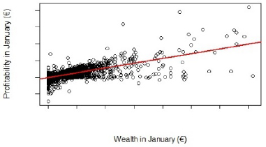
Figure 16.1. Relation between customer wealth and profitability for the bank in January
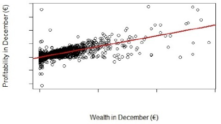
Figure 16.2. Relation between customer wealth and profitability for the bank in December
Three shortcomings of the database were made evident in a preliminary analysis. The first is related to outliers in customer profitability, which will be analyzed in section 16.3.
The second shortcoming is that the records that are interpreted as different customers may correspond to the same person who chooses to open different accounts: for example, someone who chooses to create an account for day-to-day transactions and another for retirement savings (retirement mutual funds, stock market investments and the like). Although this may create some bias, we do not expect this to happen in many cases, so the impact of such possibility will probably be limited.
Another, more serious, shortcoming is the existence of just 1 year of data, aggregated in monthly values. This makes it difficult to assess the medium- and long-term behavior of the customers, for example to determine whether or not a customer is in churn. It also makes it impossible to test medium- and long-term forecasts. This shortcoming is expected to cause some problems in the estimation of customer profitability and customer churn.
In order to assess the accuracy of prediction models, data were divided into two sets; 60% of the observations were used as a training set to estimate the models. The other 40% of the observations constitutes a test set, which was used to assess the prediction accuracy in data that was not used in the estimations.
16.3. Short-term forecasting of customer profitability
Profitability from a client in a given month is expected to be strongly correlated with the profitability in the previous month. This is clearly shown to be the case in Figure 16.3, which shows the relation between the profitability in January and February. As expected, the points in this graph are very close to the straight line y = x, showing that that profitability given by the client in a given month is a good forecast of the profitability given by the client in the next month. Therefore, we aimed at forecasting the changes in profitability instead of the profitability in order to avoid getting apparently good forecasting results just because profitability shows high persistence.
Figure 16.4 shows the relation between the profitability in June and July. Once again, the relation is close to the straight line y = x, for the large majority of observations, but there are several important outliers, corresponding to customers whose profitability shows a visible increase. In fact, in May and July, the profitability associated with some customers has an important increase, only to show a similar decrease in the following month (June and August, respectively). This introduces outliers in the data, harming the ability to predict future profitability. According to an analysis of this situation made with bank members, this seems to be due to the way the profitability of some (very few) products is accounted. New, more realistic ways of considering the profitability of these products will be analyzed with the bank but, meanwhile, we chose to use the existing values in order to avoid the risk of introducing biases in the data.
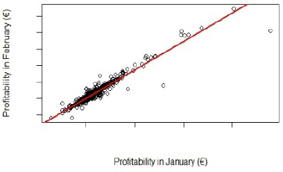
Figure 16.3. Relation between the profitability of the clients in January and February
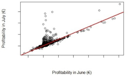
Figure 16.4. Relation between the profitability of the clients in June and July
Figure 16.5 shows a histogram with the monthly values of the profitability. We can see that there are a very large number of slightly negative values of the monthly profitability.
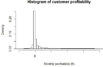
Figure 16.5. Histogram with monthly values of customer profitability
We started by trying to predict the change in customer profitability 1 month ahead. We used both sociodemographic data and data from the customer activity and balances in the three previous months to estimate the change in the customer profitability in the next month. For example, data concerning activity, transactions and balances from January, February and March, are used to estimate the change in profitability between March and April. The goodness-of-fit measure that we chose is the root mean square error (RMSE) and we compare the obtained forecast with the naïve forecast that assumes that the change in profitability is equal to the average change in the training period (termed ModAvg).
The first types of models to be estimated were linear models. This allowed us to get a first idea of the relevance of the different variables for explaining the changes in profitability. The non-relevant variables were iteratively removed and, in the end, the model presented an adjusted R2 of 0.4593. The performances of the model thus obtained and of the benchmark model (ModAvg), both in the training and in the test sets, are summarized in Table 16.1.
Table 16.1. Performance of the linear model and benchmark model
| Model | RMSE in the training set | RMSE in the test set |
| Linear model | 12.90 | 15.21 |
| ModAvg | 17.67 | 19.72 |
As can be seen in Table 16.1, the linear model is better than ModAvg, both in the training set and in the test set, and model performance deteriorates in the test set.
In order to give an idea of the impacts of the different variables, we show the sign of the coefficients and their statistical significance in Table 16.2, for some of the most significant variables. Since we are considering some data from the three previous months to estimate the change in customer profitability, the coefficient signs are presented for each of these months (1, 2 and 3 months before the change in profitability we are trying to forecast).
In some cases, the coefficient signs change from 1 month to the next, while remaining very significant. This is a clear indication that not only the value of the variable is relevant to forecast the change in profitability, but the change in the value may be relevant as well. For example, wealth in the latest month has a positive sign, whereas wealth in the month before has a negative sign: this may mean that both the most recent value of the wealth and the latest change in wealth have a positive influence in the expected change in profitability.
Table 16.2. Sign and significance of some of the most significant variables of the linear model
| Sign and significance | |||
| One month before | Two months before | Three months before | |
| Online logins | +*** | +* | – |
| Number of online transactions | +*** | –*** | –*** |
| Credit card transactions | +*** | –*** | +*** |
| Number of different mutual funds in the account | +*** | + | –*** |
| Value of stock market holdings | –*** | +*** | + |
| Number of stock market transactions | –*** | +** | –*** |
| Total wealth | +*** | –*** | –*** |
| Total value of loans | +*** | + | –*** |
| Value allocated to term deposits in the month | +*** | +*** | – |
| Value removed from term deposits in the month | –*** | –*** | –*** |
| Amount of wages deposited in the bank | +*** | –*** | +** |
| Profitability from checking account | –*** | +*** | + |
| Profitability from term deposits | –*** | +*** | + |
| Profitability from home equity loans | –*** | +*** | +*** |
| Profitability from other (non-home equity) loans | –*** | +*** | +*** |
| Profitability from mutual funds | –*** | +*** | –*** |
| Profitability from stock market holdings | –*** | +*** | + |
| Age | +*** | ||
+,–: sign of the coefficient; *significant at the 10% level; **significant at the 5% level;
***significant at the 1% level.
In the cases of stock market holdings and transactions, the coefficient signs seem to be the contrary of what was expected. One possible explanation may be that customers with larger stock market holdings use the account mostly to make trades and deposit such assets (that is as an investment account), and they do not tend to buy new products that are profitable to the bank.
Another interesting result is the negative and statistically significant sign in the last month profitability, for the different categories of products. However, this has a simple interpretation: all other things remaining constant, the larger the profitability already is, the less it is expected to increase.
Finally, note that only one sociodemographic variable is significant: age. Older clients generate more profits than younger clients. The significance of age was also found on the other models that we considered.
We also applied linear models to forecast the change of profitability at 2-, 3- and 4- month horizons. The results, shown in Table 16.3, clearly show that the forecasting ability of the models decreases when the forecasting horizon becomes longer.
Table 16.3. Performance of linear models on the test set for different forecasting horizons
| Forecasting horizon | RMSE in the training set | RMSE in the test set |
| 1 month | 12.90 | 15.21 |
| 2 months | 14.63 | 17.29 |
| 3 months | 16.39 | 18.62 |
| 4 months | 17.56 | 20.33 |
After this linear model, several data mining methods were applied: regression random forests, gradient boosting, naïve Bayes and linear discriminant analysis. Although these methods perform better than the linear model in the training set (sometimes very significantly), we could never improve the predictive performance in the test set, when compared with the linear model. So, there seems to be an overfitting problem with the application of these data mining techniques to predict profitability. However, due to the long computation times associated with the application of these techniques, we tried a limited number of configurations for each one. In random forests, for example, it is possible that a different set of variables, or different numbers of trees or of candidates to each split, might lead to better results.
16.4. Churn prediction
One important initial difficulty in churn prediction was the definition of churn. The bank had no clear definition and, for this work, we chose to define churn through rules that are mostly based on common sense: there is churn if there are no relevant products and small amounts of credits and of wealth deposited in the bank. The exact rules consisted of defining that a customer was in churn if, simultaneously, he/she had no insurance contracts, no term deposits, no mutual funds and no credit or debit cards, the wealth in the bank was below 1,000 € and the loans amounted to less than 100 €.
Our goal in predicting churn was mainly to predict which customers are not currently in churn but have a high probability of churning in the future. When we mention churning in the future, we are considering a reasonable amount of time; given the fact that we have data for only 1 year, we chose to predict churn using a 6-month horizon. In order to have enough data to try using different lags, we aimed at trying to predict which customers were not in churn in June 2015, but were in churn in December 2015. The number of customers in this situation was quite low, less than 0.7% of the customers in the database.
Churn prediction was handled as a classification problem. We used both linear models (probit and logit) and several data mining techniques (Adaboost, linear discriminant analysis, classification random forests). The best results were achieved with classification random forests, which obtained a much better performance than all the other models. We will only present the results obtained by classification random forests and logit models (the linear models with the best performance).
We started to use a large number of variables in the models, both sociodemographic and related to balances, transactions and other activity. For balances, transactions and other activity, we started by using the values from January to June 2015. We defined a variable that measures the ratio between the value of wealth in June and the average wealth in the semester, and we defined a similar variable for the amount of loans. We also defined new binary variables, for several products, to define whether or not the customer had any of that product (regardless of the amount) in each month, and also for determining whether the customer had made any online logins and transactions in each month.
Several configurations were tried (mostly in the linear models) in order to assess whether the binary variables or the initial values performed better, and then the less significant variables were iteratively removed. In the end, the number of relevant variables was much smaller than for profitability prediction. In almost all the cases, we found out that only the most recent value was relevant, the main exceptions being the two new variables that measured the relation between June values and average semester values for wealth and credits.
In general, the most relevant variables were:
- – age;
- – wealth;
- – ratio between the wealth in June and the average wealth on the semester;
- – value of loans;
- – ratio between the value of loans in June and the average value of the semester;
- – profitability in the latest months;
- – total balance of term deposits;
- – existence of transactions and logins in the latest months.
The models we used define the probability that a customer is going to churn. In order to assess the prediction ability, we calculated the average probability that the models assign to churners and to non-churners. The results are shown in Table 16.4, and they show that random forests assign much higher probabilities to customers that effectively end up churning, although they also assign slightly higher probabilities to non-churners.
Table 16.4. Performance of the best linear model (logit) and the best nonlinear technique (random forests)
| Model | Logit model | Random forest |
| Average probability assigned by the model to customers that effectively churn | 3.78% | 9.89% |
| Average probability assigned by the model to customers that end up not churning | 0.66% | 0.71% |
We can see that random forests show some ability in differentiating future churners from non-churners. However, we must acknowledge that, due to limitations in the data that were mentioned in section 16.2, we cannot be sure if the customers we are identifying as churning are, in reality, churning.
16.5. Next-product-to-buy
We also tried to predict, for some products, whether or not a given product from the bank will be the given customer’s next buy. Since data are monthly, we are in fact identifying whether customers buy a product in the next month in which they acquire one or more products from the bank. This is also a classification problem: a product is classified as whether or not it will be bought in the month a next purchase is made. We used both linear models (probit and logit) and data mining techniques (random forests, Adaboost, linear discriminant analysis).
Three products, held by an important percentage of customers, were considered: term deposits, debit cards and credit cards. Purchase of such products was identified as an increase in the number of units of the product in the customer account. This allows us to avoid incorrectly classifying as purchases the cases in which a customer just changes a product he currently holds by another of the same kind (e.g. ending a term deposit and applying the capital in a new one).
The logic used for defining the training and test sets was somewhat different in this analysis. In the training set, the prediction was made for the next purchase in the months from May to August using data from the previous three months (February to April). In the test set, we intended to predict the next purchase in the 4-month period from September to December using data from the previous 3 months (June to August). Only customers making any kind of purchase in the considered 4-month period were taken into account (i.e. we try to predict what is the next product to be bought; we are not making a joint prediction of the next product and of the probability of a buying occurring).
Apart from sociodemographic variables and transactions, balances and bank-related activity in the three previous months, new binary variables were added regarding the occurrence of purchases of the different types of products for each of the three previous months.
Table 16.5. Performance of logit models in predicting the next product bought by a customer
| Product | Percentage of customers for which the product is the next to be bought | Average probability estimated by the model when the product is the next to be bought | Average probability estimated by the model when the product is not the next to be bought | Percentage of customers correctly identified by the model as buying the product next | Percentage of customers, among the 5% with largest probability in the model for which the product is the next to be bought |
| Term deposits | 51.4% | 59.7% | 41.9% | 71.3% | 90.0% |
| Debit cards | 11.4% | 20.5% | 9.7% | 38.2% | 60.2% |
| Credit cards | 13.7% | 19.9% | 11.7% | 31.6% | 38.0% |
The best results in the test set were obtained with logit models. In Table 16.5, we present the performance of these models. In order to assess the predictive ability of the models, we considered the average probability given by the model when the product is the next to be bought and when it is not, the percentage of customers correctly identified by the model as buying the product next, and also the percentage of customers, among those with the top 5% probabilities estimated by the model, who effectively buy that product next. This last measure is particularly interesting for defining targeted marketing campaigns, since it allows the identification of the customers that will most probably buy the product. We also present the percentage of customers for which the product is the next to be bought – this is, in fact, the probability of a customer next buying that product, when you choose him/her at random.
We can see that the models perform quite well. In particular, the customers to whom the models assign higher probabilities really do have a high probability of next purchasing the product.
16.6. Conclusions and future research
In this chapter, we present the results of an analysis of churn, profitability and NPTB, obtained using a database concerning the behavior of customers from a Portuguese bank. If it is possible to accurately predict churn probabilities and the evolution of profitability, then it is possible to estimate CLV, which is of great importance for defining marketing strategies.
As we explained, the database has some shortcomings, including not identifying the same client with different accounts, the existence of profitability outliers and the fact of there being just 1 year of data, aggregated in monthly values.
A linear model showed a good performance in the estimation of future short-term profitability at the 1-month horizon, but the performance of the estimated models seems to deteriorate when the prediction horizon increases, even if it is only to a few months. For churn, we had no solid reference to determine when a customer churns, so we defined a rule for identifying churning customers. A random forest seems to have an interesting ability to forecast which customers will churn in the next 6 months. However, given the short time period covered by the database, we cannot be completely sure that the customers identified as having churned did, indeed, churn. Therefore, given the limitations in the results concerning profitability and churn prediction, we feel that it is not yet possible to make a credible calculation of CLV. Still, the results concerning churn are interesting and may help identify the customers whose relation with the bank is becoming very weak. The bank may thus target these customers with marketing campaigns in order to try to avoid losing them.
The results of the models of the NPTB are very interesting and show that a logit model has a good ability to predict the next product that a customer will buy. In particular, a large percentage of the customers to whom the model predicted the top 5% largest probabilities of purchasing each of the considered products did indeed buy that product next. This opens the way to targeted marketing campaigns for selling the products that the customers are more likely to purchase.
At the outset, we expected data mining techniques to outperform the predictive ability of linear models. Although data mining techniques usually perform much better in the training set, only in the case of churn were they able to beat a logit model in the test set. Possible explanations for this may be that linear models are particularly suited to this data set, that the shortcomings of the database are especially harming the performance of data mining techniques and that different parameterizations of the techniques should be tested in order to fine-tune them to the characteristics of the data. Concerning this latter explanation, the number of tested parameterizations was indeed limited due to very long computational running times, but we will, in the future, try new parametrizations and new approaches in order to achieve better predictions.
As future work, we are already in contact with the bank to get a database covering a longer time period. This is expected to allow us to define a more credible identification of churning customers and better predictions of future profitability and NPTB. We will also address the estimation of CLVs, both using predictions of churn probability and future profitability and also using other approaches made available by a longer database. Finally, we will try to obtain better predictions of the NPTB and propose models for defining long-term market strategies based on these predictions.
16.7. References
Ali, Ö.G., Arıtürk, U., (2014). Dynamic churn prediction framework with more effective use of rare event data: The case of private banking. Expert Syst Appl. 41(17), 7889–7903.
Blattberg, R.C., Malthouse, E.C., Neslin, S.A. (2009). Customer lifetime value: Empirical generalizations and some conceptual questions. J Interact Market. 23(2), 157–168.
Ekinci, Y., Ülengin, F., Uray, N., Ülengin, B. (2014). Analysis of customer lifetime value and marketing expenditure decisions through a Markovian-based model. European J Oper Res. 237(1), 278–288.
EsmaeiliGookeh, M., Tarokh, M.J. (2013). Customer lifetime value models: A literature survey. Int J Indust Eng. 24(4), 317–336.
Fader, P.S., Hardie, B.G., Lee, K.L. (2005). “Counting your customers” the easy way: An alternative to the Pareto/NBD model. Market Sci. 24(2), 275–284.
Fader, P.S., Hardie, B.G., Lee, K.L. RFM, CLV: Using iso-value curves for customer base analysis. J. Market Res. 42(4), 415–430.
Fader, P.S., Hardie, B.G., Shang, J. (2010). Customer-base analysis in a discrete-time noncontractual setting. Market Sci. 29(6), 1086–1108.
Glady, N., Baesens, B., Croux, C. (2009). A modified Pareto/NBD approach for predicting customer lifetime value. Expert Syst Appl. 36(2), 2062–2071.
Haenlein, M., Kaplan, A.M., Beeser, A.J. (2007). A model to determine customer lifetime value in a retail banking context. Eur Manage J. 25(3), 221–234.
He, B., Shi, Y., Wan, Q., Zhao. X. (2014). Prediction of customer attrition of commercial banks based on SVM model. Procedia Comput Sci. 31, 423–430.
Knott, A., Hayes, A., Neslin, S.A. (2002). Next-product-to-buy models for cross-selling applications. Journal of Interact Market. 16(3), 59–75.
Li, S., Sun, B., Montgomery, A.L. (2011). Cross-selling the right product to the right customer at the right time. J Market Res. 48(4), 683–700.
Li, S., Sun, B., Wilcox, R.T. (2005). Cross-selling sequentially ordered products: An application to consumer banking services. J Market Res. 42(2), 233–239.
Mzoughia, M.B., Limam, M. (2015). An improved customer lifetime value model based on Markov chain. Appl Stoch Models Bus Industry 31(4), 528–535.
Schmittlein, D.C., Morrison, D.G., Colombo, R. (1987). Counting Your Customers: Who-Are They and What Will They Do Next? Manage Sci. 33(1), 1–24.
Schmittlein, D.C., Peterson, R.A. (1994). Customer base analysis: An industrial purchase process application. Market Sci. 13(1), 41–67.
Singh, S.S., Jain, D.C. (2010). Measuring customer lifetime value. Rev Market Res. 6, 37–62.
Chapter written by Pedro GODINHO, Joana DIAS and Pedro TORRES.