9

Building Data Models at the Physical Level

Tableau relationships are the preferred way to bring multiple tables together in Tableau Desktop. We learned about relationships in Chapter 8. There are some cases where you, the data modeler, need to be one level deeper. For these use cases, we must go to the physical layer of the data source. We can get to this level by creating a join or using custom SQL.

When we create a join, Tableau creates a new table that results from the joining of the two tables. The structure of the new table depends on the type of join we use. We will be studying the four join options in this chapter. These are left join, right join, inner join, and full or outer join. In addition to joins, we will explore custom SQL statements and demonstrate the impact of using both versus using relationships.

In this chapter, we’re going to cover the following topics:

• Opening relationships to join at the physical layer through database joins
• Geospatial joins and using the intersects operator with a BUFFER calculation
• Using joins to create a data model with row-level security
• Understanding custom SQL – when to use it and the pitfalls of using it

Technical requirements

For the complete list of requirements to run the practical examples in this chapter, please see the Technical requirements section in Chapter 1.

All the exercises and images in this chapter will be described using the Tableau Desktop client software except where noted. You can also recreate all the exercises in this chapter using the Tableau web client, which has a very similar experience to the Desktop client.

To run the exercises in this chapter, we will need the following downloaded files:

• Superstore Sales Orders - US.xlsx
• Product Database.xlsx
• Sales Argentina.csv
• Bicycle_Thefts.csv
• toronto_crs84.geojson

The files we will be using are based on Superstore data, the sample data that Tableau uses in its products. The exception will be the bicycle thefts and Toronto neighborhood shapefiles. These files came from https://data.torontopolice.on.ca/ and https://www.toronto.ca/city-government/data-research-maps/open-data/ respectively.

The files used in the exercises in this chapter can be found at https://github.com/PacktPublishing/Data-Modeling-with-Tableau/.

Opening relationships to join at the physical layer through database joins

Before Tableau released the relationships feature, the only way to expand your analysis to use additional fields from a secondary table in Tableau was to create a join at the physical layer of the data.

Although relationships are the preferred method of combining tables to get additional fields, joins still have their use cases.

Cases where you might use joins are as follows:

• When you know you are only supporting one use case in the Tableau workbook(s) that uses the model
• When you want to filter data through your join
• When you need to use an entity table for row-level security
• When you are making a geospatial join

Let’s start by exploring the first two use cases, supporting a single use case and using the join for data filtering.

Single use case and using the join for a filter

When exploring joins in Chapter 8, we looked back to Chapter 4, when we joined the sales data with the product data. We will continue to use these two tables in this join example.

Imagine that you have been tasked with providing analysis for the sales team. They want to know how sales have been affected by priority, product category and sub-category, shipping option, and other dimensions. They never need to ask the question, “what didn’t sell?” That is a task they leave for the marketing team. They are also not concerned with the task of uncovering bad data. They only want facts on what sold over time.

Let’s create our join for this use case:

1. Open Tableau Desktop. When you open Tableau Desktop you will see the Connect pane on the left-hand side of the user interface. From the Connect pane, under the To a File section, select Microsoft Excel. Locate the Superstore Sales Orders - US.xlsx file, select it, and click on Open. We should now be looking at a screen as shown in Figure 9.1:

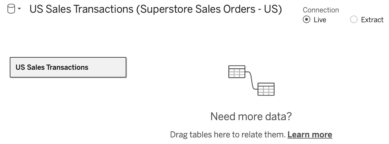
Figure 9.1 – Tableau data source page after connecting to US Sales

2. Next, we need to join our product information. Click on the Add link to the right of Connections. Under the To a File section, select Microsoft Excel. Locate the Product Database.xlsx file, select it, and click on Open.
3. Our screen should now look like the screenshot in Figure 9.2. We now have two data sources in our workbook, namely Superstore Sales Orders – US and Product Database. The Product Database.xlsx file also only has a single sheet. This sheet is called Product DB:

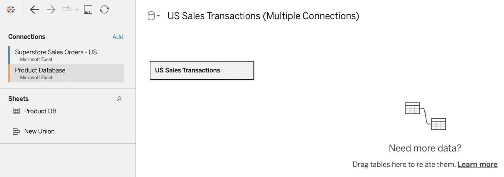
Figure 9.2 – Data source page with Product DB added

4. This is where things get different from relationships. If we drag Product DB to the canvas, Tableau will show us the noodle and will try to create a relationship. To create a join, we first have to open our US Sales Transactions table. Hover on the right side of the US Sales Transactions card and when the ▼ symbol appears, click on it and choose Open as seen in Figure 9.3:

Figure 9.3 – Open on a table in the canvas

5. Drag the Product DB table to the right of US Sales Transactions and release the left mouse button to drop the table. Your canvas should now look like the screenshot in Figure 9.4:

Figure 9.4 – US Sales Transactions joined to Product DB

6. Instead of the noodle, we notice that we get a Venn diagram of two overlapping circles. This represents our join at the physical layer. The default is an inner join. Let’s first look at this join type. Click on the Venn diagram and notice the join diagram as seen in Figure 9.5:

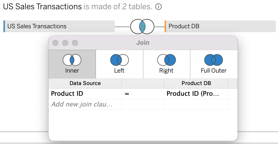
Figure 9.5 – Join diagram

We can see that we have four different join choices:

• Inner – This is a join where the resulting table will only contain records that exist in both the left and right table where the join fields/join clauses match
• Left – This is a join where the resulting table will contain all the records in the left table and only the records from the right table where the rows contain a matching record on the join fields/join clauses
• Right – This is a join where the resulting table will contain all the records in the right table and only the records from the left table where the rows contain a matching record on the join fields/join clauses
• Full Outer – This is a join where the resulting table will contain all the records of both tables

7. Let’s see what happens when we create an inner join between these tables. Leave the inner join selected and close the join dialog box. Click on Sheet 1 to begin. Under the US Sales Transactions table, double-click Sales to bring it into the view. Under the Product DB table, double-click to bring Product Name into the view. To make it easier to get to our answer to which product sold the most, click on the Swap Rows and Columns icon in the toolbar then click on the Sort Descending button. Hover on the bar for the top item. You should now have a view that looks like Figure 9.6:

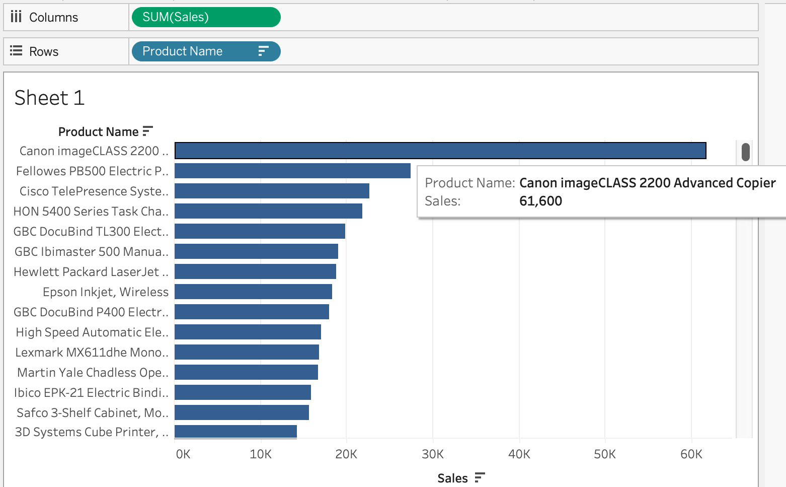
Figure 9.6 – Result of inner join of sales and product tables

8. The inner join worked to both apply the filter to eliminate the two bad product IDs from the sales table and answer the question of which products brought in the most sales. When we created a relationship between these tables in Chapter 8, we had to filter out the bad records. In addition to helping us find those records, it also allowed us to answer the question of which products did not sell. We can’t get that answer from this inner join because products that did not sell are not in the new table that results from our join. To conclude with the inner join, it works well when you know you want to both filter out unmatched records and only need to answer questions that can be answered by records that match in both tables. It eliminates choice and flexibility in analysis, but there are cases where that is preferred. This inner join would work if we were building our data model for a sales team that is only concerned about sales of products from our product database. Less data also means faster queries, so it is a good idea to bring in only the data needed for analysis.
9. Let’s now look at the left join of the same table. Click on the Data Source tab to go back to the data source page. Click on the Venn diagram for our join and then click on the icon for Left join. Your screen should now look like Figure 9.7:

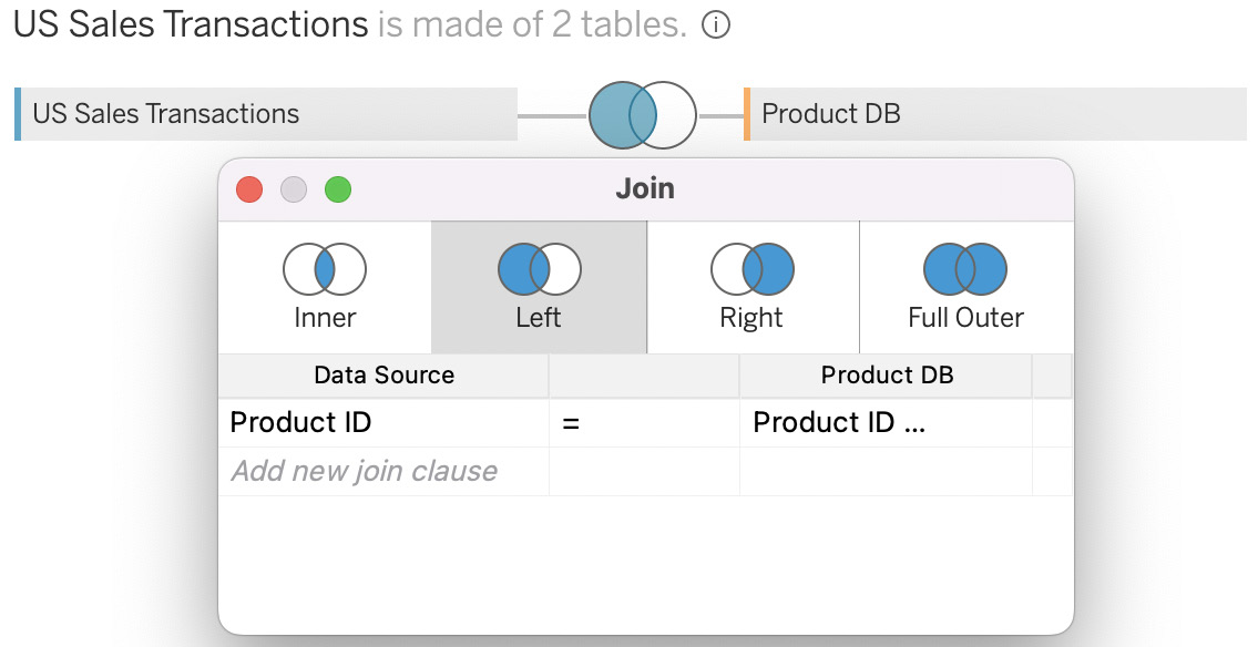
Figure 9.7 – Create a left join

10. Click to dismiss the join dialog. Click on Sheet 1 and notice how the chart has changed. We now have a long bar, representing a lot of sales, associated with a Null product name. Drag and drop the Product ID field from the US Sales Transactions table to the right of Product Name on the Rows shelf. Your screen should now look like Figure 9.8:

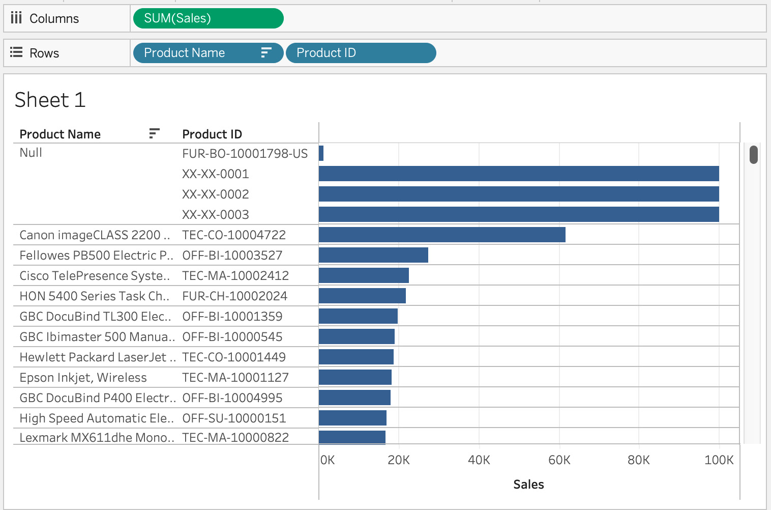
Figure 9.8 – Result of a left join

11. We notice that we have four product IDs that are in our sales (left) table but aren’t in our product database (right) table. For this reason, the left join type kept the records from the sales table even though it couldn’t find a match in the product database. Just like our similar exercise with relationships in Chapter 8, we could filter these out of our view by excluding them or by using a data source or extract filter. We can see how the inner join of step 8 eliminates the need for these filters as it filters the data at the time of the join.
12. We will now look at the effect of a right join. Click on the Data Source tab to go back to the data source page. Click on the Venn diagram for our join and then click on the icon for Right join. Your screen should now look like Figure 9.9:

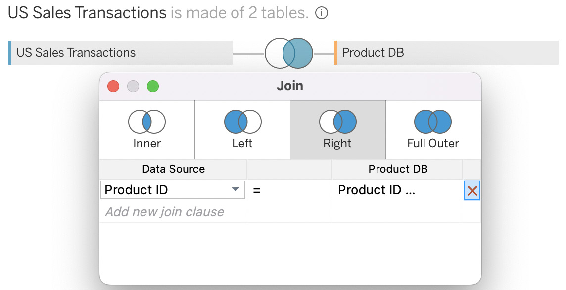
Figure 9.9 – Create a right join

13. Click to dismiss the join dialog. Click on Sheet 1. Remove the Product ID field by dragging it off the view and releasing the mouse button. Notice how the chart is the same as the inner join result except we can see >2K nulls in the bottom right-hand corner of the chart as seen in Figure 9.10. This represents the product names that we haven’t sold as we have gotten all those records from the product database (right) table. We don’t see the null product names as they only existed in the sales (left) table. In this case, the right join gives us the answer to which products have and have not sold. It does not allow us to answer the question of which sales we had that did not have a product in our product database.

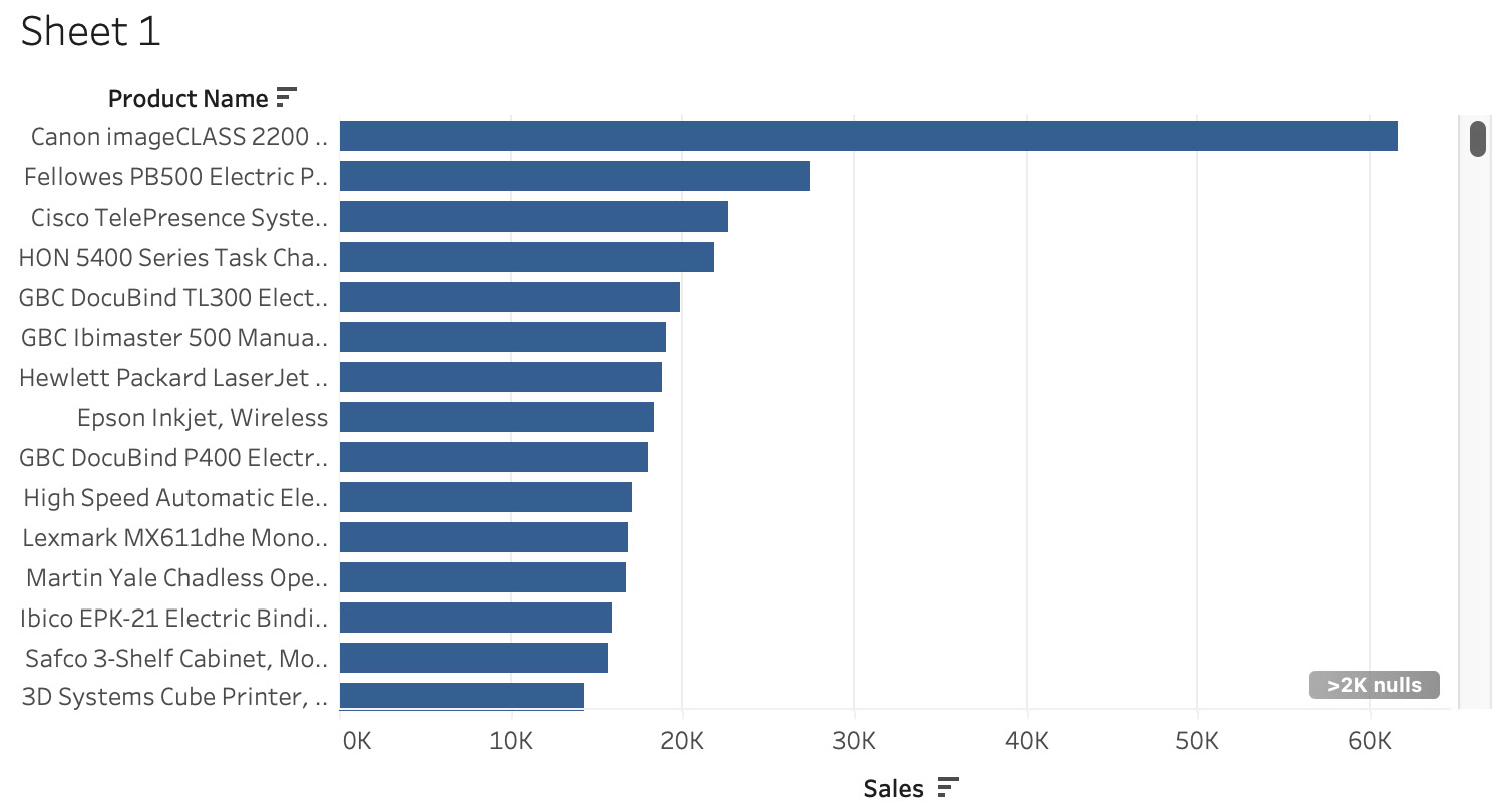
Figure 9.10 – Results of a right join

14. The final join type that we could do is a Full Outer join. This join type would bring in all records from both tables, joining on Product ID where it matched. It would also bring in all the records from both tables where there was no match for Product ID. This might seem the same as a relationship, but the big difference is that a relationship only queries the table or tables it needs to answer the question posed in Tableau. With a full outer join, the single table Tableau creates will be much larger than the combination of the two tables individually. In addition, the unmatched records will have null values for all the fields of the corresponding table as there were no rows to match. Having a lot of null values will lead to longer query response times and can make analysis difficult.

In this section, we looked at the four join types in Tableau and how they differed from relationships. We demonstrated each of the four and compared them to the results we saw with the same data tables with relationships in Chapter 8. In the next section, we will look at using geospatial joins.

Geospatial join type to drive map-based analysis

Tableau has a lot of built-in capabilities for geospatial analysis. In addition to the built-in capabilities, it is possible to bring in geospatial files to enhance this type of analysis. We connected to a geospatial file in Chapter 7. In this section, we are going to join a geospatial file with a text file that contains information on bike thefts in the city of Toronto, Ontario, Canada.

The question we are going to answer is, “which Toronto neighborhoods have the highest number of bicycle thefts?”:

1. Open Tableau Desktop. When you open Tableau Desktop you will see the Connect pane on the left-hand side of the user interface. From the Connect pane, under the To a File section, select Text file, find the Bicycle_Thefts.csv file that you downloaded from GitHub, and click OK.
2. Click on Sheet 1 and then double-click on Latitude followed by double-clicking on Longitude. Make sure you click on the Latitude and Longitude fields from the table and not the Latitude (generated) and Longitude (generated) fields that are in italics. You should now see a map that looks like Figure 9.11. This map shows a single value, which is the average latitude and longitude in our dataset:

Figure 9.11 – Average latitude and longitude for bike thefts in Toronto

3. To make this analysis meaningful, we need to add detail to our view. Drag and drop the Event Unique ID field on the Details mark card and drag and drop the Neighbourhood Name field on the Color mark card, as shown in Figure 9.12. Now we have a bit of an idea of which neighborhoods have the most bicycle thefts, but it isn’t as clear as it could be. We can’t realistically count all those dots!

Figure 9.12 – Unique crimes by neighborhood

4. To make the answer to our question clearer, we can use a geospatial file that has the shape of Toronto neighborhoods in it. Click on the Data Source tab. Click on Add in the connection pane. Choose To a File | Spatial File, select toronto_crs84.geojson, and click OK. Click on the ▼ symbol next to Bicycle_Thefts.csv in the canvas and choose Open for the table per Figure 9.13:

Figure 9.13 – Open bicycle thefts

5. Drag the toronto_crs84.geojson table onto the canvas to create an Inner join. On the left side (bicycle thefts) of the join, click Add new join clause and then select Create Join Calculation… as seen in Figure 9.14:

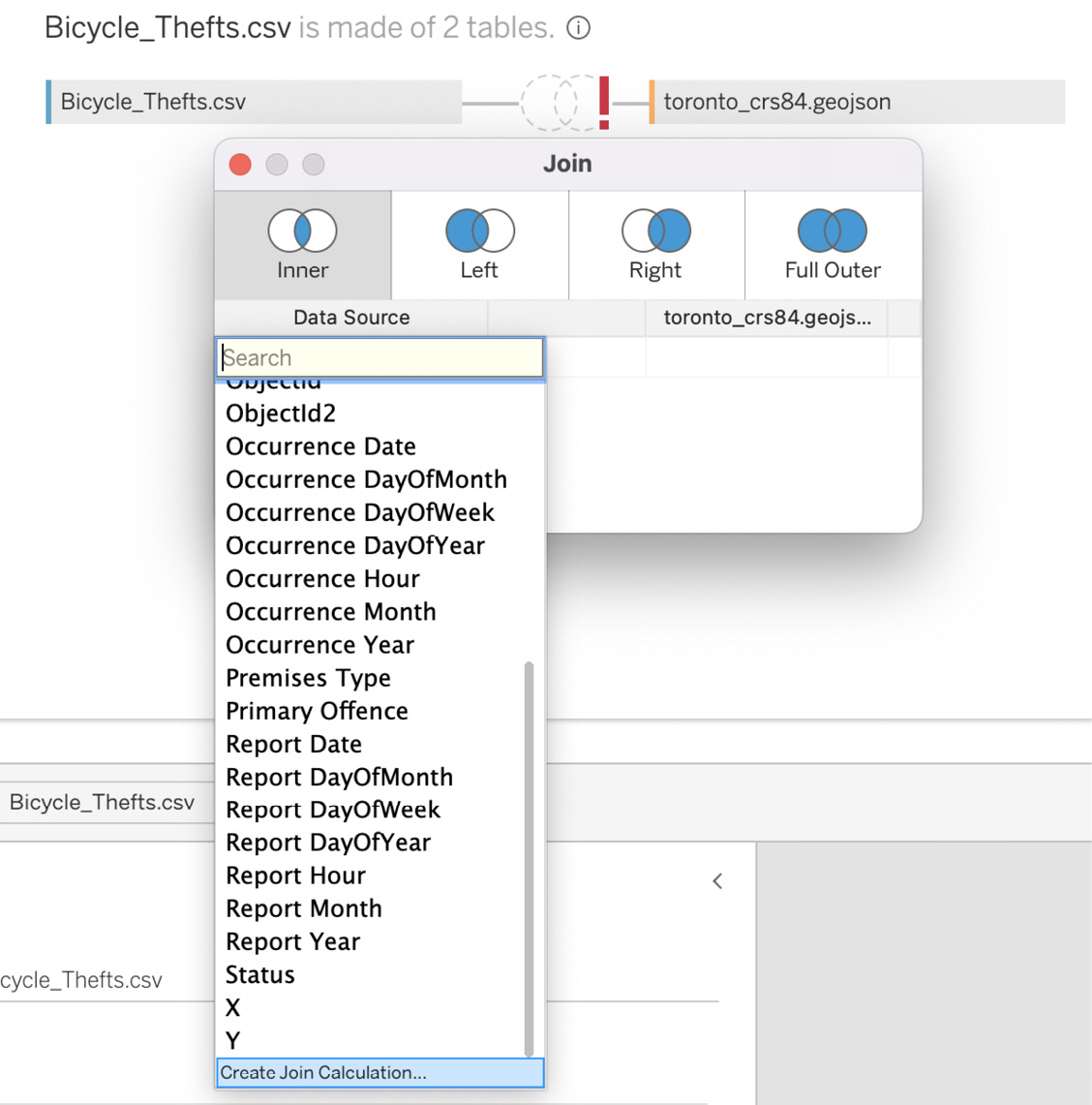
Figure 9.14 – Create Join calculation

6. In the calculation dialog box, enter MAKEPOINT([Latitude], [Longitude]) and click OK as in Figure 9.15. The reason for this calculation is that we need a single field for our join. MAKEPOINT allows us to do this with our latitude and longitude fields:

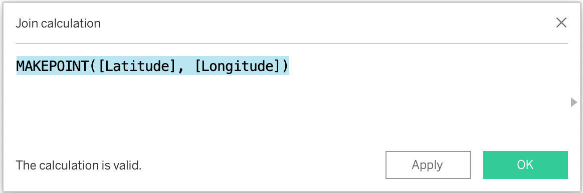
Figure 9.15 – MAKEPOINT calculation

7. To complete our join, click on the join clause on the right table (toronto_crs84.geojson) and choose the Geometry field. Choose Intersects for the join operator. Intersects is a unique join operator for geospatial joins. It tells Tableau to join records from the left table if the latitude and longitude fall within the boundaries of the Geometry field of the right table. This option does not exist with relationships, which is why we need to use joins for combining geospatial files. We can see the join in Figure 9.16:

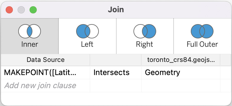
Figure 9.16 – Geospatial join

8. To see how this enhances our analysis, click the new worksheet icon to the right of Sheet 1 to create Sheet 2. From Sheet 2, double-click on the Geometry field under the toronto_crs84.geojson table in the data pane. Your screen should now look like Figure 9.17, showing the outlines of Toronto’s neighborhoods:

Figure 9.17 – Toronto neighborhoods

9. To complete our viz, drag and drop the Neighbourhood Name field on the Detail marks card. Drag the Event Unique ID field on the Color marks card. This will result in a very colorful map but it doesn’t help us with what we are looking to answer. Right-click on the Event Unique ID field in the cards shelf and select Measure | Count (Distinct) as per Figure 9.18:

Figure 9.18 – Convert Event Unique ID to a measure

10. This now gives us the view showing where the most bicycle thefts occurred. The darker the color, the greater the number of thefts, as seen in Figure 9.19:

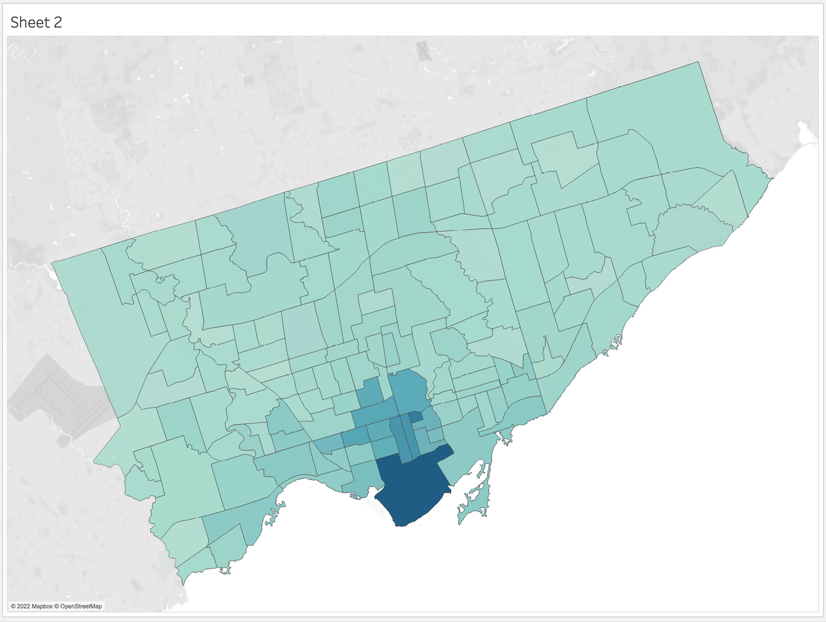
Figure 9.19 – Map showing where most bicycle thefts occur

In this section, we created a geospatial join to analyze data using maps. When we need to make a combination of fields to perform a geospatial analysis, we need to use a join as we can’t use a relationship for this type of analysis. In the next section, we will discuss the use case of using joins with entity tables to achieve row-level security.

Using joins to create a data model with row-level security

There are several ways to implement row-level security in our Tableau data model. We will be looking at these in detail in Chapter 11. For the purposes of this chapter, it is worth noting that one method is to have a separate table with usernames in it joined to the data table at the row level based on the user who is signed into Tableau Server or Cloud. We bring it up here as a use case for joins versus relationships. This technique only works with joins – your data would not be secure if you used a relationship, as this could be used to generate a query from the data table without joining to check entitlements to the data.

We will look at custom SQL in the next and final section of this chapter.

Understanding custom SQL – when to use it and the pitfalls of using it

After we create our data models using relationships or joins, and analysts begin to interact with the data, Tableau dynamically creates SQL code to retrieve the data needed for the analyses. Tableau also goes beyond SQL with its proprietary query language called VizQL. VizQL adds additional features to SQL queries that also tells Tableau what chart type to use based on the data results from the query. Tableau does not expose the SQL and VizQL code it generates. It is all generated behind the scenes.

It is possible for us to write our own SQL in our data models using custom SQL. If we are connected to a data server that supports SQL queries, we will see a New Custom SQL option at the bottom of the tables from our database, as shown in Figure 9.20. Current versions of Tableau do not support custom SQL with Microsoft Excel:

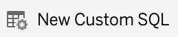
Figure 9.20 – New Custom SQL option

After double-clicking on New Custom SQL, you are able to type your SQL query into a Notepad-like textbox and save it. It will then appear on your canvas like any table you import, as shown in Figure 9.21. You can create relationships with it and joins within it as with any other table in Tableau:

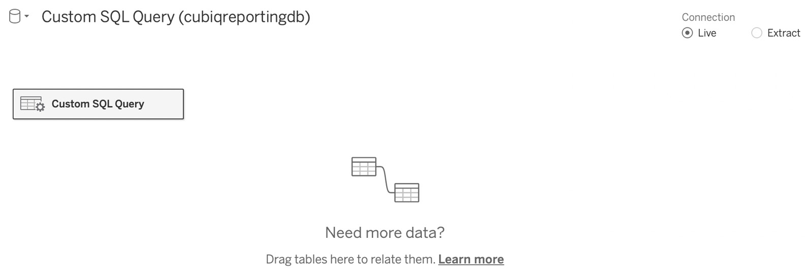
Figure 9.21 – Canvas with a custom SQL query

The temptation to use custom SQL is high if we are comfortable writing SQL and new to Tableau. However, it is usually a good idea to avoid custom SQL whenever we can. The reason relates to the first paragraph of this section. Tableau dynamically creates VizQL, and the SQL associated with it. When we use custom SQL, Tableau always uses it as a sub-query. In other words, Tableau wraps the dynamic SQL it creates around the custom SQL query. This often has a negative impact on query performance and dashboard load time. If you have a use case that requires custom SQL, it is a better idea to create a table or view in the database and bring the resulting table into Tableau. Tableau can then create more efficient queries.

This does not mean it is never a good idea to use custom SQL. If you cannot get the database results you want from Tableau without creating a custom SQL statement, create the custom SQL statement and determine whether the load and query times for your data source and workbooks are fast enough. If performance is acceptable, you can continue to use the custom SQL tables without needing to create a new view or table in the database.

In this section, we discussed how Tableau dynamically creates SQL within its proprietary VizQL language. We learned that we can also create our own custom SQL queries to generate tables in Tableau. We also learned that we should avoid custom SQL when we can because Tableau always uses our custom SQL as subqueries, which can have a negative impact on performance.

Summary

We explored building data models at the physical layer of our data sources in this chapter. We do this by creating joins between the tables in our data model.

We looked at left, right, inner, and full outer joins and how to create them by opening tables in the Tableau canvas. We created a geospatial join using the Intersects operator, something that is not possible with relationships.

Another use case for using joins over relationships that we covered is to create a data model with row-level security using a security table of usernames joined to the data that we want to secure.

In the final section of the chapter, we explored custom SQL within the scope of how Tableau dynamically creates SQL, concluding that we should use custom SQL sparingly.

In the next chapter, we will be looking at extending and sharing data models and when to use live connections versus extracts.