Chapter 2. Exploring the Dataset
In the previous chapter, we’ve talked about how you can ingest your data into the cloud, and run some ad-hoc queries with Athena as well as Redshift.
We also had a first peak into our dataset. As we’ve learned, the Amazon Customer Reviews dataset consists of more than 130+ million of those customer reviews of products across 43 different product categories on the Amazon.com website from 1995 until 2015.
The dataset contains the actual customer reviews text together with additional metadata, and is shared in both a tab separated value (TSV) text format, as well as in the optimized columnar binary format Parquet.
Here is the schema for the dataset again:
- marketplace
-
2-letter country code (in this case all “US”).
- customer_id
-
Random identifier that can be used to aggregate reviews written by a single author.
- review_id
-
A unique ID for the review.
- product_id
-
The Amazon Standard Identification Number (ASIN). http://www.amazon.com/dp/<ASIN> links to the product’s detail page.
- product_parent
-
The parent of that ASIN. Multiple ASINs (color or format variations of the same product) can roll up into a single parent parent.
- product_title
-
Title description of the product.
- product_category
-
Broad product category that can be used to group reviews (in this case digital videos).
- star_rating
-
The review’s rating (1 to 5 stars).
- helpful_votes
-
Number of helpful votes for the review.
- total_votes
-
Number of total votes the review received.
- vine
-
Was the review written as part of the Vine program?
- verified_purchase
-
Was the review from a verified purchase?
- review_headline
-
The title of the review itself.
- review_body
-
The text of the review.
- review_date
-
The date the review was written.
In the next sections of this chapter, we will explore and visualize the dataset in more depth, and introduce some tools and services that assist you in this task.
Overview
Query services like Athena, data warehouses like Redshift, Jupyter notebooks like SageMaker Notebooks, data processing engines like EMR, and dashboard and visualization tools like QuickSight, all address different use cases. Of course, you should choose the right tool for the right purpose. This chapter describes the breadth and depth of tools available within AWS, and maps these tools to common use cases seen across our customer base.
In the previous chapter, we already introduced you to Athena and Redshift.
-
Amazon Athena offers ad-hoc, serverless SQL queries for data in S3 without needing to setup, scale, and manage any clusters.
-
Amazon Redshift provides the fastest query performance for enterprise reporting and business intelligence workloads, particularly those involving extremely complex SQL with multiple joins and subqueries across many data sources including relational databases and flat files.
In this chapter, we will also start to use Jupyter notebooks as our main workspace and development environment.
-
Amazon SageMaker Notebooks are provided via fully managed compute instances which run the Jupyter Notebook App. With just a couple of clicks, you can provision such a notebook instance and start using Jupyter notebooks to run ad-hoc data analysis, preparation and processing, as well as model development as we will see here in a bit.
To interact with AWS resources from within a Python Jupyter notebook, we leverage the AWS Python SDK boto3, the Python DB client PyAthena to connect to Athena, and SQLAlchemy) as a Python SQL toolkit to connect to Redshift.
Note
AWS Data Wrangler is an open source toolkit from Amazon to facilitate data movement between Pandas and AWS services such as S3, Athena, Redshift, Glue, EMR, etc. Many AWS best practices are built into this library.
In addition to those services, we also have Amazon Elastic MapReduce (EMR) and Amazon QuickSight available.
-
Amazon EMR supports flexible, highly-distributed, data-processing and analytics frameworks such as Hadoop and Spark when compared to on-premises deployments. Amazon EMR is flexible so you can run custom jobs with specific compute, memory, and storage parameters to optimize your analytics requirements.
-
Amazon QuickSight is a fast, easy-to-use business intelligence service to build visualizations, perform ad-hoc analysis, and build dashboards from many data sources - and across many devices.
Let’s explore our dataset in more depth now.
Visualize our Data Lake with Athena
At this point, we will shift over to use SageMaker Notebooks based on Jupyter to query and visualize our data in S3.
Amazon SageMaker is a fully managed service that provides developers and data scientists with a platform to build, train, and deploy their machine learning models. SageMaker aims at removing the heavy lifting from each step of the machine learning process to make it easier and faster to develop high quality models.
In this section, we will start working with Amazon SageMaker which provides managed Jupyter notebooks that you can start working with in minutes.
Note
For more detailed instructions on how to setup Amazon SageMaker Notebooks in your AWS account, please refer to Appendix C - Setup Amazon SageMaker.
Prepare SageMaker Notebook for Athena
For our exploratory data analysis in this Jupyter notebook, we will use Pandas, NumPy, Matplotlib and Seaborn, which are probably the most commonly used libraries for data analysis and data visualization in Python. Seaborn is built on top of matplotlib and adds support for pandas.
We will also introduce you to PyAthena, the Python DB Client for Amazon Athena, that enables us to run Athena queries right from our notebook. So let’s get started by installing the mentioned libraries as follows:
%%bash
pip install -q pandas==0.23.0
pip install -q numpy==1.14.3
pip install -q matplotlib==3.0.3
pip install -q seaborn==0.8.1
pip install -q PyAthena==1.8.0
We also need to import a couple more libraries, one of them is boto3. Boto is the Amazon Web Services (AWS) SDK for Python. It enables Python developers to create, configure, and manage AWS services. Boto provides an easy to use, object-oriented API, as well as low-level access to AWS services.
We use boto3 to identify the AWS region we’re currently working in, and use the pre-installed Amazon SageMaker Python SDK (sagemaker) to configure and interact with the service. Let’s also define the database and table holding our Amazon Customer Reviews dataset information in Amazon Athena.
import boto3
import sagemaker
import numpy as np
import pandas as pd
import seaborn as sns
import matplotlib.pyplot as plt
%matplotlib inline
%config InlineBackend.figure_format='retina'
session = boto3.session.Session()
region_name = session.region_name
sagemaker_session = sagemaker.Session()
bucket = sagemaker_session.default_bucket()
database_name = 'dsoaws'
table_name = 'amazon_reviews_parquet'
With that, we are now ready to run our first SQL queries right from the notebook.
Note
If you are on a Mac, make sure you specify the retina setting above for retina-resolution images in Matplotlib. The difference is stunning!
Run a Sample Athena Query in the SageMaker Notebook
In the first example shown below, we will query our dataset to give us a list of the distinct product categories. PyAthena uses a connection cursor to connect to the data source, execute the query and store the query results in S3.
-
connect returns a cursor configured with our region and a S3 bucket to save query results to, our s3_staging_bucket
-
cursor.execute will execute our SQL query and store the results in CSV file format in the defined s3_staging_bucket
Note
There are different cursor implementations that you can use. While the standard cursor fetches the query result row by row, the PandasCursor will first save the CSV query results in the S3 staging directory, then read the CSV from S3 in parallel down to your Pandas DataFrame. This leads to better performance than fetching data with the standard cursor implementation. You can use the PandasCursor by specifying the cursor_class with the connect method or connection object.
# PyAthena imports
from pyathena import connect
from pyathena.pandas_cursor import PandasCursor
from pyathena.util import as_pandas
# Set S3 staging directory
# This is a temporary directory used for Athena queries
s3_staging_dir = 's3://{0}/athena/staging'.format(bucket)
# Execute query using connection cursor
cursor = connect(region_name=region_name, s3_staging_dir=s3_staging_dir).cursor()
cursor.execute("""
SELECT DISTINCT product_category from {0}.{1}
ORDER BY product_category
""".format(database_name, table_name))
We can now have a look at the results by reading the query results stored in a CSV file in our S3 staging bucket into a pandas dataframe as shown below:
# Load query results into Pandas DataFrame and show results
df_categories = as_pandas(cursor)
df_categories
The output should look similar to this:
| product_category | product_category (continued) |
| Apparel | Luggage |
| Automotive | Major Appliances |
| Baby | Mobile_Apps |
| Beauty | Mobile_Electronics |
| Books | Music |
| Camera | Musical Instruments |
| Digital_Ebook_Purchase | Office Products |
| Digital_Music_Purchase | Outdoors |
| Digital_Software | PC |
| Digital_Video_Download | Personal_Care_Appliances |
| Digital_Video_Games | Pet Products |
| Electronics | Shoes |
| Furniture | Software |
| Gift Card | Sports |
| Grocery | Tools |
| Health & Personal Care | Toys |
| Home | Video |
| Home Entertainment | Video DVD |
| Home Improvement | Video Games |
| Jewelry | Watches |
| Kitchen | Wireless |
| Lawn and Garden |
Note
As common with Pandas DataFrames, PandasCursor handles the data on memory. Pay attention to the file size when reading data into the DataFrame. You can easily exceed your available memory when working with large datasets.
Dive Deep into the Dataset with Athena and SageMaker
Let’s use Athena, SageMaker Notebooks, Matplotlib, and Seaborn to track down answers to the following questions over the entire dataset:
-
Which product categories are the highest rated by average rating?
-
Which product categories have the most reviews?
-
When did each product category become available in the Amazon catalog based on the date of the first review?
-
What is the breakdown of star ratings (1-5) per product category?
-
How have the star ratings changed over time? Is there a drop-off point for certain product categories throughout the year?
-
Which star ratings (1-5) are the most helpful?
Note
From this point, we will only show the Athena query and the results. The full source code to execute and render the results is available in the accompanying GitHub repo.
-
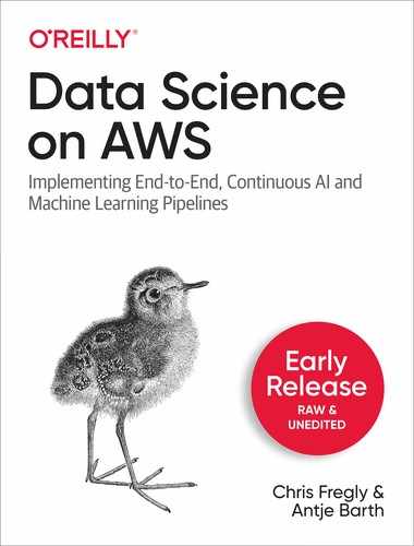
Which product categories are the highest rated by average rating?
SELECT product_category, AVG(star_rating) AS avg_star_rating
FROM dsoaws.amazon_reviews_parquet
GROUP BY product_category
ORDER BY avg_star_rating DESC
Let’s plot this in a horizontal bar chart using Seaborn and Matplotlib.
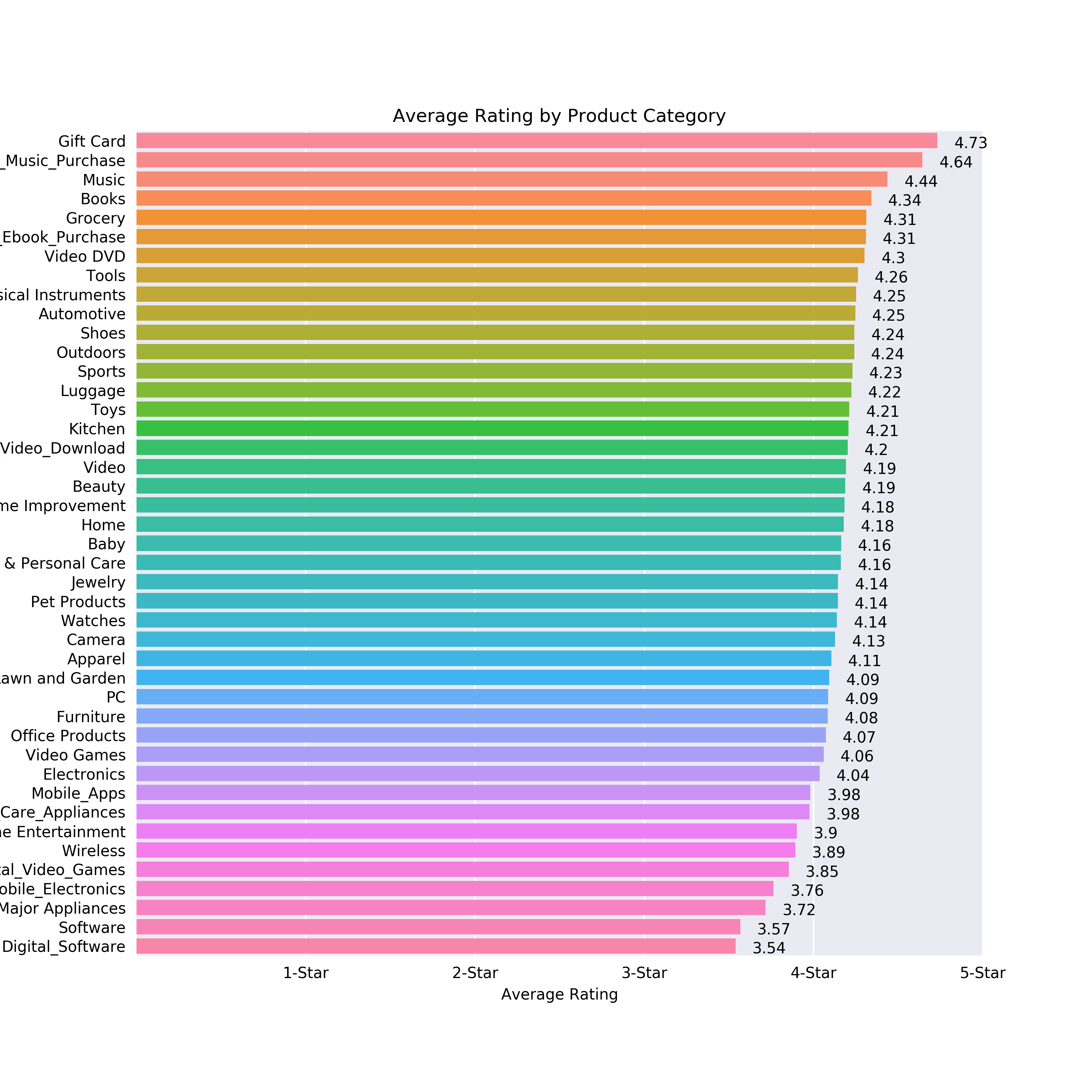
Figure 2-1. Horizontal bar chart showing average rating per category
-
As we can see in Figure 4-1, Amazon Gift Cards are the highest rated product category with an average star rating of 4.73, followed by Music Purchase with an average of 4.64 and Music with an average of 4.44.
-
Which product categories have the most reviews?
SELECT product_category, COUNT(star_rating) AS count_star_rating FROM dsoaws.amazon_reviews_parquet
GROUP BY product_category
ORDER BY count_star_rating DESC
-
Let’s plot this again in a horizontal bar chart using Seaborn and Matplotlib.
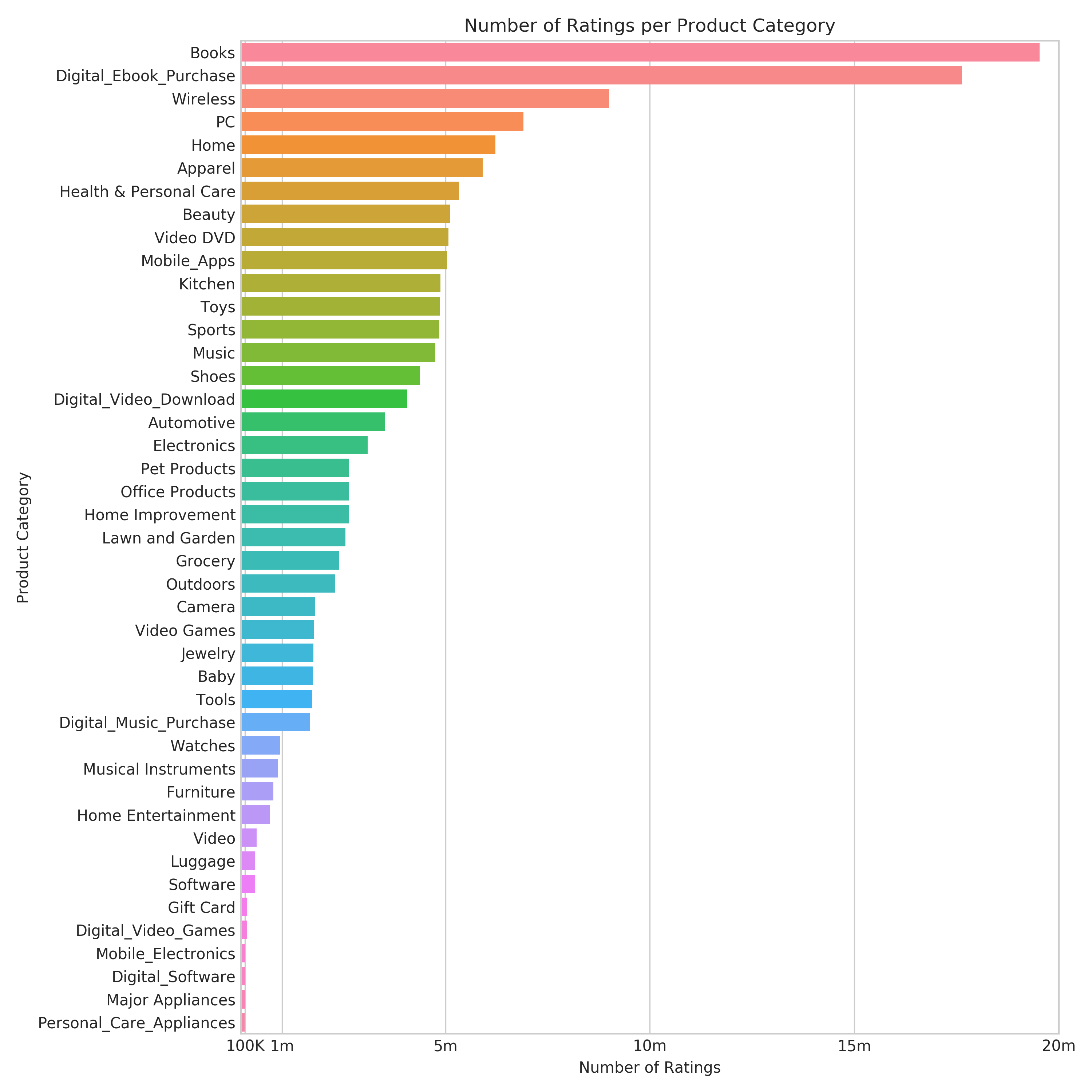
Figure 2-2. Horizontal bar chart showing number of reviews per category.
-
We can see in Figure 4-2 that the “Books” product category has the most reviews with close to 20 million. This makes sense as Amazon.com initially launched as the “Earth’s Biggest Bookstore” back in 1995 as shown in a restored picture of Amazon.com’s first website in Figure 2-3.

Figure 2-3. Amazon.com Website, 1995 (Source: Version Museum)
-
The second most reviewed category is “Digital_Ebook_Purchase” representing Kindle book reviews. So we notice that book reviews - whether printed or as ebooks - still count the most reviews.
-
“Personal_Care_Appliances” has the least number of reviews. This could potentially be due to the fact that the product category got added more recently.
-
Let’s check this out by querying for the first review in each category which will give us a rough timeline of product category introductions.
-
When did each product category become available in the Amazon catalog?
-
The initial review date is a strong indicator of when each product category went live on Amazon.com.
SELECT product_category, MIN(DATE_FORMAT(DATE_ADD('day', review_date, DATE_PARSE('1970-01-01','%Y-%m-%d')), '%Y-%m-%d')) AS first_review_date FROM amazon_reviews_tsv GROUP BY product_category ORDER BY first_review_date -
The result should look similar to this:
product_category first_review_date Books 1995-06-24 Music 1995-11-11 Video 1995-11-11 Video DVD 1996-07-08 Toys 1997-01-05 Sports 1997-10-09 Video Games 1997-11-06 Home 1998-05-29 Office Products 1998-07-15 Pet Products 1998-08-23 Software 1998-09-21 Home Entertainment 1998-10-15 Camera 1998-11-20 Wireless 1998-12-04 Health & Personal Care 1999-02-06 Outdoors 1999-03-24 Electronics 1999-06-09 PC 1999-07-01 Baby 1999-07-13 Digital_Ebook_Purchase 1999-08-28 Grocery 1999-09-05 Automotive 1999-10-24 Shoes 1999-11-08 Home Improvement 1999-11-08 Tools 1999-11-09 Lawn and Garden 1999-11-27 Musical Instruments 1999-12-13 Kitchen 2000-01-20 Furniture 2000-03-17 Digital_Music_Purchase 2000-06-28 Major Appliances 2000-08-26 Apparel 2000-09-06 Digital_Video_Download 2000-10-04 Personal_Care_Appliances 2000-10-29 Beauty 2000-10-31 Watches 2001-04-05 Jewelry 2001-11-10 Mobile_Electronics 2001-12-22 Luggage 2002-11-05 Gift Card 2004-10-14 Digital_Video_Games 2006-08-08 Digital_Software 2008-01-26 Mobile_Apps 2010-11-04 -
We can see that personal care appliances were indeed added somewhat later to the Amazon.com catalog, but that doesn’t seem to be the only reason for the low number of reviews. Mobile apps appear to have been added around 2010.
-
Let’s visualize the number of first reviews per category per year, shown in Figure 4-4

Figure 2-4. Number of first product category reviews per year.
-
We notice that a lot of our first product category reviews (13) happened in 1999. Whether this is really related to the introduction of those product categories around this time, or just a coincidence created by the available data in our dataset, we can’t tell for sure.
-
What is the breakdown of ratings (1-5) per product category?
SELECT product_category, star_rating, COUNT(*) AS count_reviews FROM dsoaws.amazon_reviews_parquet GROUP BY product_category, star_rating ORDER BY product_category ASC, star_rating DESC, count_reviews -
The result should look similar to this (shortened):
product_category star_rating count_reviews Apparel 5 3320566 Apparel 4 1147237 Apparel 3 623471 Apparel 2 369601 Apparel 1 445458 Automotive 5 2300757 Automotive 4 526665 Automotive 3 239886 Automotive 2 147767 Automotive 1 299867 ... ... ... -
With this information, we can also quickly group by star ratings and count the reviews for each rating (5, 4, 3, 2, 1):
SELECT star_rating, COUNT(*) AS count_reviews FROM dsoaws.amazon_reviews_parquet GROUP BY star_rating ORDER BY star_rating DESC, count_reviews -
The result should look similar to this:
star_rating count_reviews 5 93200812 4 26223470 3 12133927 2 7304430 1 12099639 -
Approximately 62% of all reviews have a 5 star rating. We will come back to this relative imbalance of star ratings when we perform feature engineering to prepare for model training.
-
We can now calculate and visualize a stacked percentage horizontal bar plot, showing the proportion of each star rating per product category.
SELECT product_category, star_rating, COUNT(*) AS count_reviews FROM {}.{} GROUP BY product_category, star_rating ORDER BY product_category ASC, star_rating DESC, count_reviews -
In Figure 4-5 you see the visualization of the breakdown by star rating:

Figure 2-5. Distribution of reviews per star rating (5, 4, 3, 2, 1) per product category.
-
We see that 5 and 4 star ratings make up the largest proportion within each product category. But let’s see if we can spot differences in product satisfaction over time.
-
How have the star ratings changed over time? Is there a drop-off point for certain product categories throughout the year?
-
Let’s first have a look at the average star rating across all product categories over the years:
SELECT year, ROUND(AVG(star_rating), 4) AS avg_rating
FROM dsoaws.amazon_reviews_parquet
GROUP BY year
ORDER BY year;
-
The result should look similar to this:
year avg_rating 1995 4.6169 1996 4.6003 1997 4.4344 1998 4.3607 1999 4.2819 2000 4.2569 2001 4.1954 2002 4.1568 2003 4.1104 2004 4.057 2005 4.0614 2006 4.0962 2007 4.1673 2008 4.1294 2009 4.1107 2010 4.069 2011 4.0516 2012 4.1193 2013 4.1977 2014 4.2286 2015 4.2495 -
If we plot this as shown in Figure 4-6, we notice the general upwards trend with two lows in 2004 and 2011.

Figure 2-6. Average Star Rating across all product categories over the years
-
Let’s have a look now at our top 5 product categories by number of ratings ('Books', ‘Digital_Ebook_Purchase', ‘Wireless', ‘PC’ and ‘Home').
SELECT product_category, year, ROUND(AVG(star_rating), 4) AS avg_rating_category FROM dsoaws.amazon_reviews_parquet WHERE product_category IN ('Books', 'Digital_Ebook_Purchase', 'Wireless', 'PC', 'Home') GROUP BY product_category, year ORDER BY year -
The result should look similar to this (shortened):
product_category year avg_rating_category Books 1995 4.6111 Books 1996 4.6024 Books 1997 4.4339 Home 1998 4.4 Wireless 1998 4.5 Books 1998 4.3045 Home 1999 4.1429 Digital_Ebook_Purchase 1999 5.0 PC 1999 3.7917 Wireless
...1999
...4.1471
... -
If we plot this now as shown in Figure 2-7, we can see something interesting:
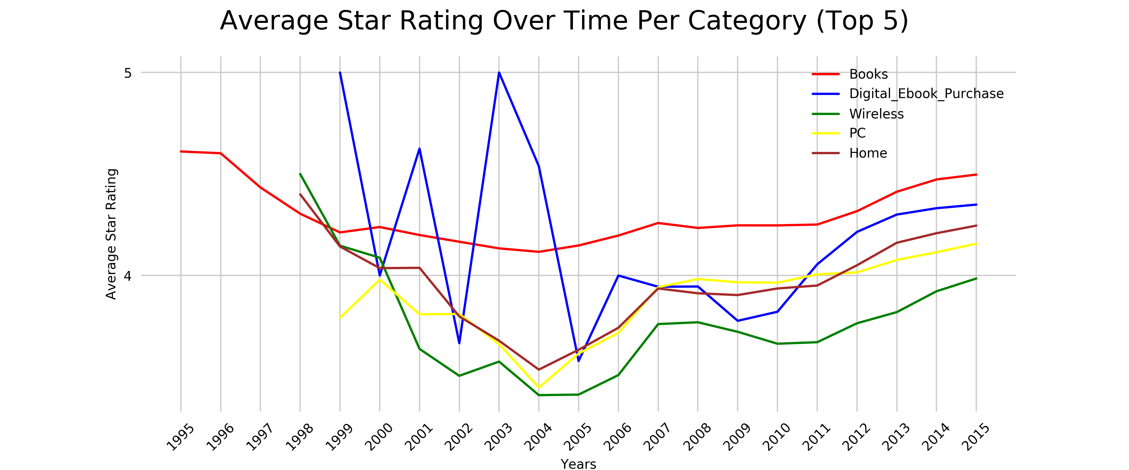
Figure 2-7. Average Star Rating Over Time Per Category
-
While books have been relatively consistent in star ratings, and stick between 4.1 and 4.6, the other categories are more affected by customer satisfaction. The Digital_Ebooks_Purchase (Kindle books) seem to spike a lot with dropping as low as 3.5 in 2005, while at 5.0 in 2003. This would definitely require a closer look into our dataset, to decide whether this is due to limited reviews in that time or some sort of skewed data, or really reflecting the voice of our customers.
-
Which star ratings (1-5) are the most helpful?
SELECT star_rating, AVG(helpful_votes) AS avg_helpful_votes FROM dsoaws.amazon_reviews_parquet GROUP BY star_rating ORDER BY star_rating DESC -
The result should look similar to this:
star_rating avg_helpful_votes 5 1.672697561905362 4 1.6786973653753678 3 2.048089542651773 2 2.5066350146417995 1 3.6846412525200134 -
We see that customers find negative reviews more helpful than positive reviews, also visualized in Figure 2-8 below.
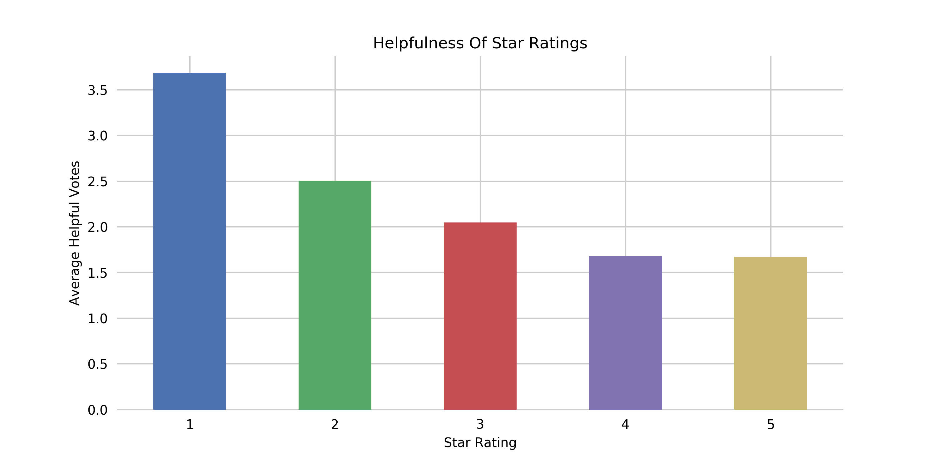
Figure 2-8. Helpfulness Of Star Ratings.
In the next section, we will show you how to query our data warehouse from Jupyter notebooks.
Query our Data Warehouse
At this point, we will use Redshift to query and visualize some use cases. Similar to the previous example with Athena, we first need to prepare our SageMaker Notebook environment again.
Prepare SageMaker Notebook for Redshift
We need to install SQLAlchemy, define our Redshift connection parameters, query the Redshift secret credentials from AWS Secret Manager, and obtain our Redshift Endpoint address. Finally, create the Redshift Query Engine.
# Install SQLAlchemy
!pip install -q SQLAlchemy==1.3.13
# Redshift Connection Parameters
redshift_schema = 'redshift'
redshift_cluster_identifier = 'dsoaws'
redshift_host = 'dsoaws'
redshift_database = 'dsoaws'
redshift_port = '5439'
redshift_table_2015 = 'amazon_reviews_tsv_2015'
redshift_table_2014 = 'amazon_reviews_tsv_2014'
# Load the Redshift Secrets from Secrets Manager
import json
import boto3
secretsmanager = boto3.client('secretsmanager')
secret = secretsmanager.get_secret_value(SecretId='dsoaws_redshift_login')
cred = json.loads(secret['SecretString'])
redshift_username = cred[0]['username']
redshift_pw = cred[1]['password']
redshift = boto3.client('redshift')
response = redshift.describe_clusters(ClusterIdentifier=redshift_cluster_identifier)
redshift_endpoint_address = response['Clusters'][0]['Endpoint']['Address']
# Create Redshift Query Engine
from sqlalchemy import create_engine
engine = create_engine('postgresql://{}:{}@{}:{}/{}'.format(redshift_username, redshift_pw, redshift_endpoint_address, redshift_port, redshift_database))
We are now ready to fire up our first Redshift query from the notebook.
Run a Sample Redshift Query from the SageMaker Notebook
In the example shown below, we will query our dataset to give us the number of unique customers per product category. We can use the Pandas read_sql_query function to run our SQLAlchemy query and store the query result in a Pandas dataframe.
df = pd.read_sql_query("""
SELECT product_category, COUNT(DISTINCT customer_id) as num_customers
FROM {}.{}
GROUP BY product_category
ORDER BY num_customers DESC
""".format(redshift_schema, redshift_table_2015), engine)
You can now simply print the first ten results with df:
df.head(10)
The output should look similar to this:
| product_category | num_customers |
| Wireless | 1979435 |
| Digital_Ebook_Purchase | 1857681 |
| Books | 1507711 |
| Apparel | 1424202 |
| Home | 1352314 |
| PC | 1283463 |
| Health & Personal Care | 1238075 |
| Beauty | 1110828 |
| Shoes | 1083406 |
| Sports | 1024591 |
We can see that the Wireless product category has the most unique customers providing reviews, followed by the Digital_Ebook_Purchase and Books category. We are all set now to query Redshift for some deeper customer insights.
Dive Deep into the Dataset with Redshift and SageMaker
Now, let’s query our data from 2015 in Redshift for deeper insight into our customer , and find answers to the following questions:
-
Which product categories had the most reviews in 2015?
-
Which products had the most helpful reviews in 2015? How long are those reviews?
-
What is the breakdown of star ratings (1-5) per product category in 2015?
-
How did the star ratings change during 2015? Is there a drop-off point for certain product categories throughout the year?
-
Which customers have written the most helpful reviews in 2015? And how many reviews have they written? Across how many categories? What is their average star rating?
-
Which customers are abusing the review system in 2015 by repeatedly reviewing the same product more than once? What was their average star rating for each product?
Note
Similar to the Athena examples before, we will only show the Redshift SQL query and the results. The full source code to execute and render the results is available in the accompanying GitHub repo.
Let’s run the queries and find out the answers!
-
Which product categories had the most reviews in 2015?
SELECT year, product_category, COUNT(star_rating) AS count_star_rating FROM redshift.amazon_reviews_tsv_2015 GROUP BY product_category, year ORDER BY count_star_rating DESC, year DESC -
The result should look similar to this (shortened):
year product_category count_star_rating 2015 Digital_Ebook_Purchase 4533519 2015 Wireless 2998518 2015 Books 2808751 2015 Apparel 2369754 2015 Home 2172297 2015 Health & Personal Care 1877971 2015 PC 1877971 2015 Beauty 1816302 2015 Digital_Video_Download 1593521 2015
...Sports
...1571181
... -
We notice that books are still the most reviewed product categories, but it’s actually the eBooks (Kindle books) now.
-
Let’s visualize this in a horizontal barplot as shown in Figure 2-9.
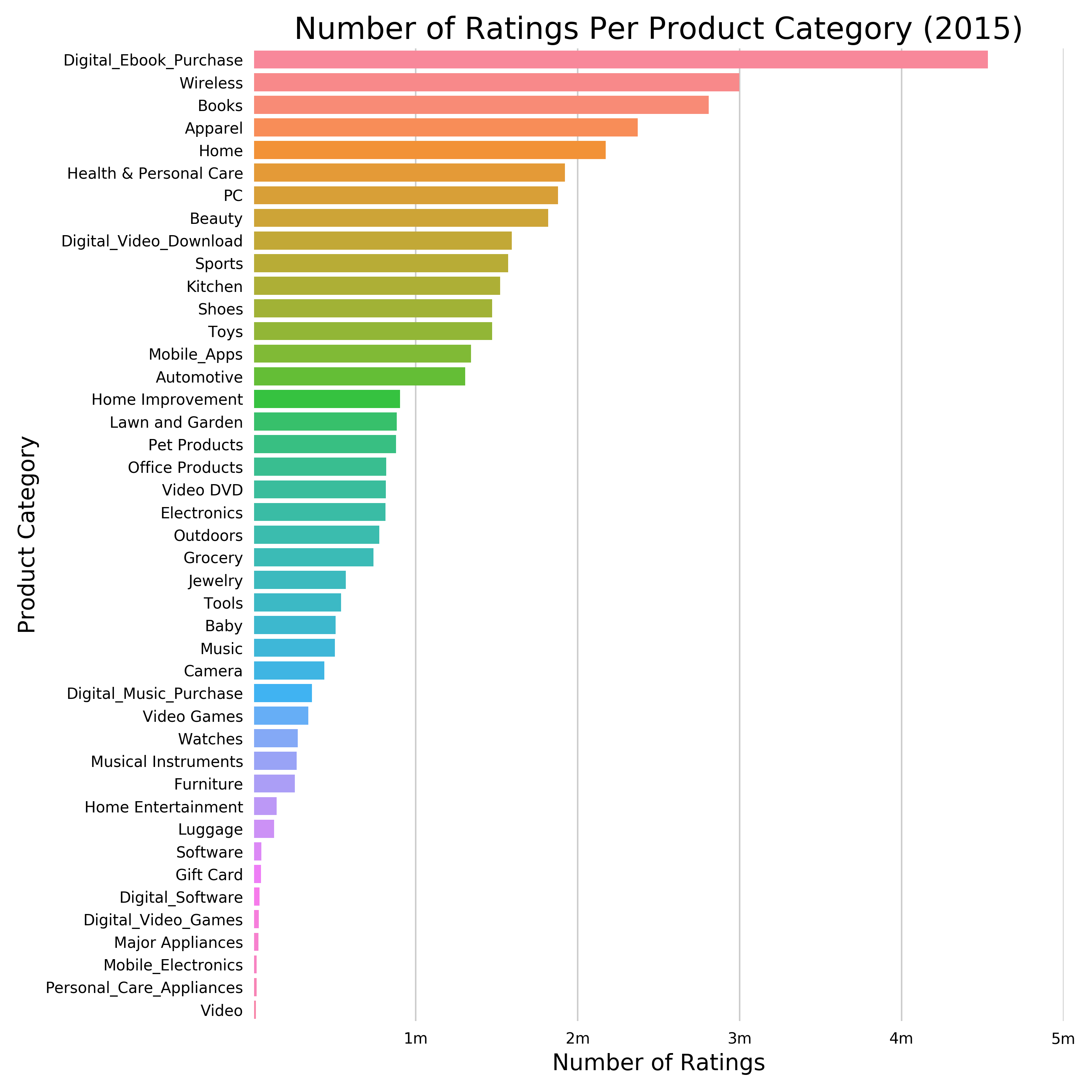
Figure 2-9. Number of Ratings Per Product Category (2015)
-
Which products had the most helpful reviews in 2015? How long are those reviews?
SELECT product_title, helpful_votes, LENGTH(review_body) AS review_body_length, SUBSTRING(review_body, 1, 100) AS review_body_substring FROM redshift.amazon_reviews_tsv_2015 ORDER BY helpful_votes DESC LIMIT 10 -
The result should look similar to this:
product_title helpful_votes review_body_length review_body_substring Fitbit Charge HR Wireless Activity Wristband 16401 2824 Full disclosure, I ordered the Fitbit Charge HR only after I gave up on Jawbone fulfilling my preord Kindle Paperwhite 10801 16338 Review updated September 17, 2015<br /><br />As a background, I am a retired Information Systems pro Kindle Paperwhite 8542 9411 [[VIDEOID:755c0182976ece27e407ad23676f3ae8]]If you’re reading reviews of the new 3rd generation Pape Weslo Cadence G 5.9 Treadmill 6246 4295 I got the Weslo treadmill and absolutely dig it. I’m 6’2", 230 lbs. and like running outside (ab Haribo Gummi Candy Gold-Bears 6201 4736 It was my last class of the semester, and the final exam was worth 30% of our grade.<br />After a la FlipBelt - World’s Best Running Belt & Fitness Workout Belt 6195 211 The size chart is wrong on the selection. I’ve attached a photo so you can see what you really need. Amazon.com eGift Cards 5987 3498 I think I am just wasting time writing this, but this must have happened to someone else. Something Melanie’s Marvelous Measles 5491 8028 If you enjoyed this book, check out these other fine titles from the same author:<br /><br />Abby’s Tuft & Needle Mattress 5404 4993 tl;dr: Great mattress, after some hurdles that were deftly cleared by stellar customer service. The Ring Wi-Fi Enabled Video Doorbell 5399 3984 First off, the Ring is very cool. I really like it and many people that come to my front door (sale -
We see that the ‘Fitbit Charge HR Wireless Activity Wristband’ had the most helpful review in 2015 with a total of 16401 votes, and a decent, yet not too long review text of 2824 characters. It’s followed by two reviews for the ‘Kindle Paperwhite’ where people were writing longer reviews of 16338 and 9411 characters respectively.
-
What is the breakdown of star ratings (1-5) per product category in 2015?
SELECT product_category, star_rating, COUNT(DISTINCT review_id) AS count_reviews FROM redshift.amazon_reviews_tsv_2015 GROUP BY product_category, star_rating ORDER BY product_category ASC, star_rating DESC, count_reviews -
The result should look like this (shortened):
product_category star_rating count_reviews Apparel 5 1350943 Apparel 4 445152 Apparel 3 245475 Apparel 2 143557 Apparel 1 184627 Automotive 5 889297 Automotive 4 177546 Automotive 3 81205 Automotive 2 49870 Automotive
...1
...106957
... -
Let’s visualize this again in a stacked percentage horizontal bar chart as shown in figure 4-10 below:
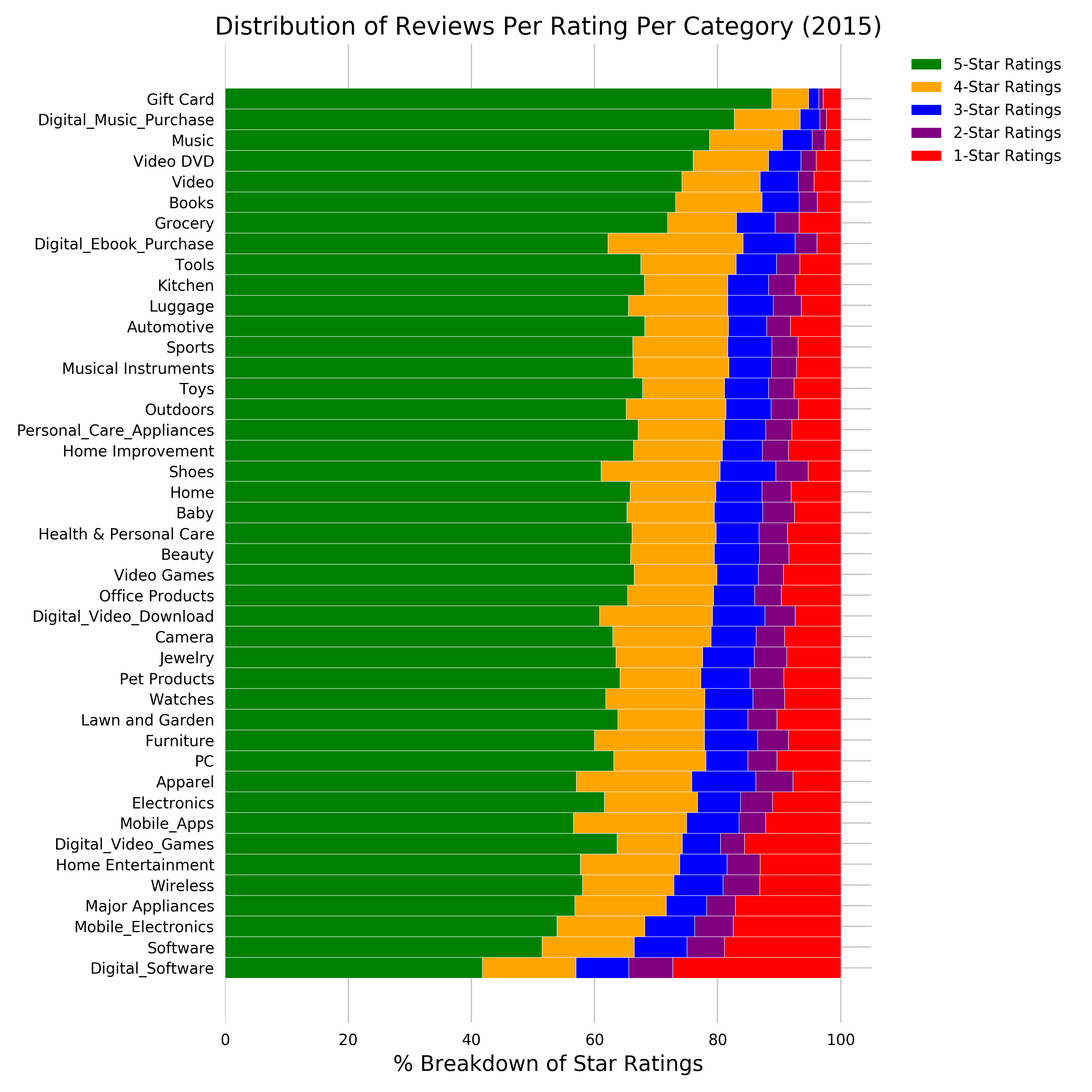
Figure 2-10. Distribution of star ratings (1-5) per product category in 2015.
-
How did the star ratings change during 2015? Is there a drop-off point for certain product categories throughout the year?
SELECT CAST(DATE_PART('month', TO_DATE(review_date, 'YYYY-MM-DD')) AS INTEGER) AS month, AVG(star_rating::FLOAT) AS avg_rating FROM redshift.amazon_reviews_tsv_2015 GROUP BY month ORDER BY month -
The result should look similar to this:
month avg_rating 1 4.277998926134835 2 4.267851231035101 3 4.261042822856084 4 4.247727865199895 5 4.239633709986397 6 4.235766635971452 7 4.230284081689972 8 4.231862792031927 -
We notice that we only have data until August 2015. We can also spot that the average rating is slowly declining, as you can easily spot in the visualization in figure 4-11 below. Assuming this data was current, the business should look into the root cause of this decline.
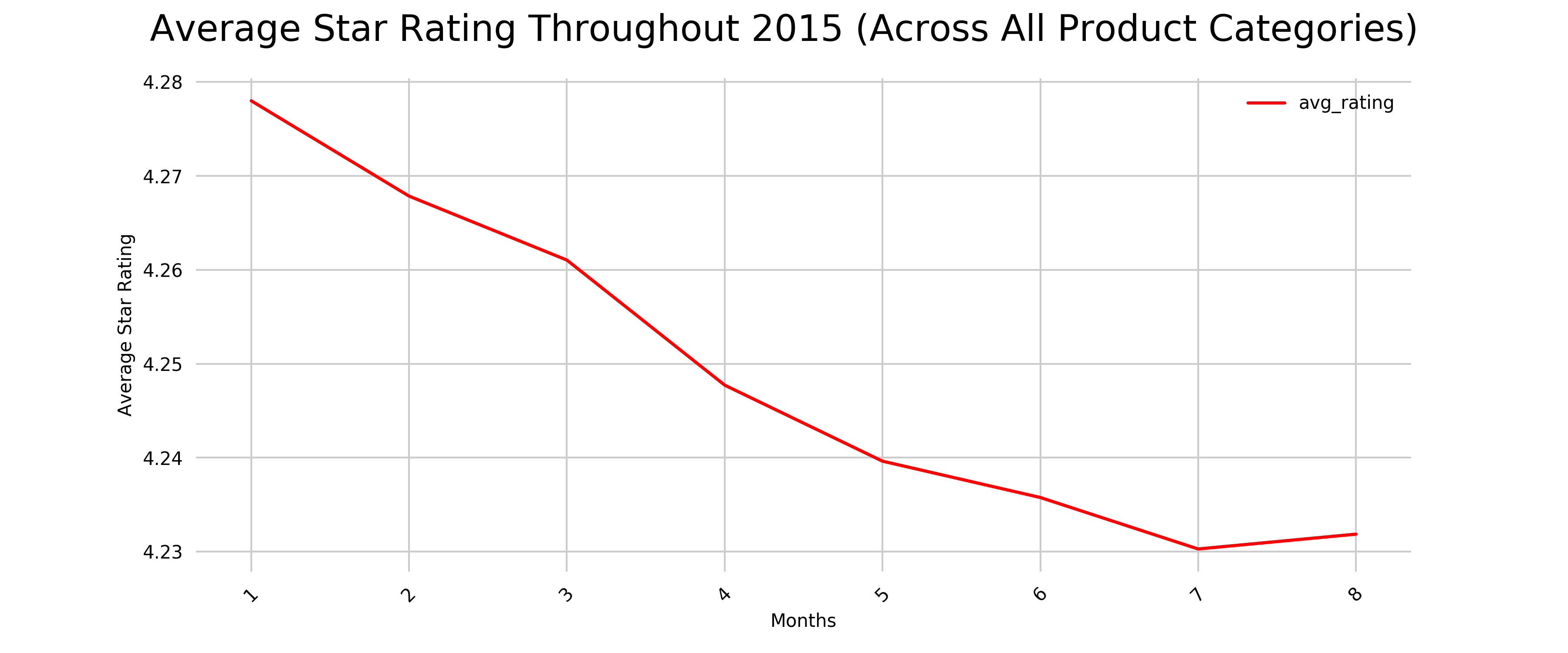
Figure 2-11. Average Star Rating Throughout 2015 (August) Across All Product Categories.
-
Now let’s explore if this is due to a certain product category dropping drastically in customer satisfaction, or more of a trend across all categories.
SELECT product_category, CAST(DATE_PART('month', TO_DATE(review_date, 'YYYY-MM-DD')) AS INTEGER) AS month, AVG(star_rating::FLOAT) AS avg_rating FROM redshift.amazon_reviews_tsv_2015 GROUP BY product_category, month ORDER BY product_category, month -
The result should look similar to this (shortened)
product_category month avg_rating Apparel 1 4.159321618698804 Apparel 2 4.123969612021801 Apparel 3 4.109944336469443 Apparel 4 4.094360325567125 Apparel 5 4.0894595692213125 Apparel 6 4.09617799917213 Apparel 7 4.097665115845663 Apparel 8 4.112790034578352 Automotive 1 4.325502388403887 Automotive 2 4.318120214368761 ... ... ... -
Let’s visualize this to see the trends easier as shown in Figure 2-12 below:
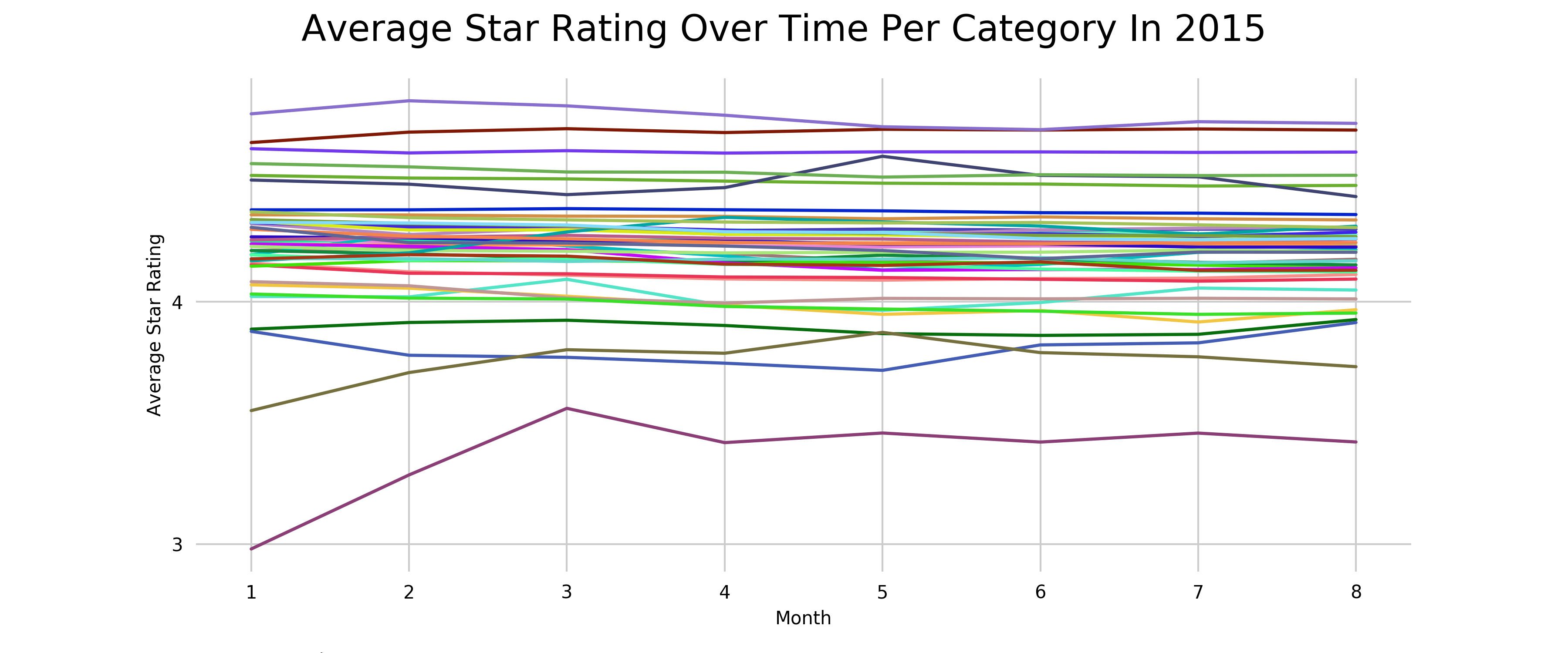
Figure 2-12. Average Star Rating over time per product category in 2015.
-
We can indeed see that most categories follow the same average star rating over the months, with just 3 categories fluctuating more (but actually improving over the year) - it’s Digital Software, Software, and Mobile Electronics.
-
Which customers have written the most helpful reviews in 2015? And how many reviews have they written? Across how many categories? What is their average star rating?
SELECT customer_id, AVG(helpful_votes) AS avg_helpful_votes, COUNT(*) AS review_count, COUNT(DISTINCT product_category) AS product_category_count, ROUND(AVG(star_rating::FLOAT), 1) AS avg_star_rating FROM redshift.amazon_reviews_tsv_2015 GROUP BY customer_id HAVING count(*) > 100 ORDER BY avg_helpful_votes DESC LIMIT 10; -
The result should look similar to this:
customer_id avg_helpful_votes review_count product_category_count avg_star_rating 35360512 48 168 26 4.5 52403783 44 274 25 4.9 28259076 40 123 7 4.3 15365576 37 569 30 4.9 14177091 29 187 15 4.4 28021023 28 103 18 4.5 20956632 25 120 23 4.8 53017806 25 549 30 4.9 23942749 25 110 22 4.5 44834233 24 514 32 4.4 -
We can see that our customers which provided the most helpful votes (with more than 100 reviews provided) review across many different categories and are generally rating with a positive sentiment.
-
Which customers are abusing the review system in 2015 by repeatedly reviewing the same product more than once? What was their average star rating for each product?
SELECT customer_id, product_category, product_title, ROUND(AVG(star_rating::FLOAT), 4) AS avg_star_rating, COUNT(*) AS review_count FROM redshift.amazon_reviews_tsv_2015 GROUP BY customer_id, product_category, product_title HAVING COUNT(*) > 1 ORDER BY review_count DESC LIMIT 5 -
The result should look similar to this:
customer_id product_category product_title avg_star_rating review_count 2840168 Camera (Create a generic Title per Amazons guidelines) 5.0 45 9016330 Video Games Disney INFINITY Disney Infinity: Marvel Super Heroes (2.0 Edition) Characters 5.0 23 10075230 Video Games Skylanders Spyro’s Adventure: Character Pack 5.0 23 50600878 Digital_Ebook_Purchase The Art of War 2.35 20 10075230 Video Games Activision Skylanders Giants Single Character Pack Core Series 2 4.85 20 -
Note where the avg_star_rating is not always a whole number. This means some customers rated the product differently over time.
-
It’s good to know that customer 9016330 finds the Disney Infinity: Marvel Super Heroes Video Game to be 5 stars - even after playing it 23 times! While customer 50600878 has been fascinated by reading The Art of War 20 times, but is still struggling to find a positive sentiment there.
Create Dashboards with QuickSight
Amazon QuickSight is an easy-to-use business analytics service which you can leverage to quickly build powerful visualizations. QuickSight automatically discovers the data sources in your AWS account including MySQL, Salesforce, Amazon Redshift, Athena, S3, Aurora, RDS, and many more as shown in Figure 2-13.
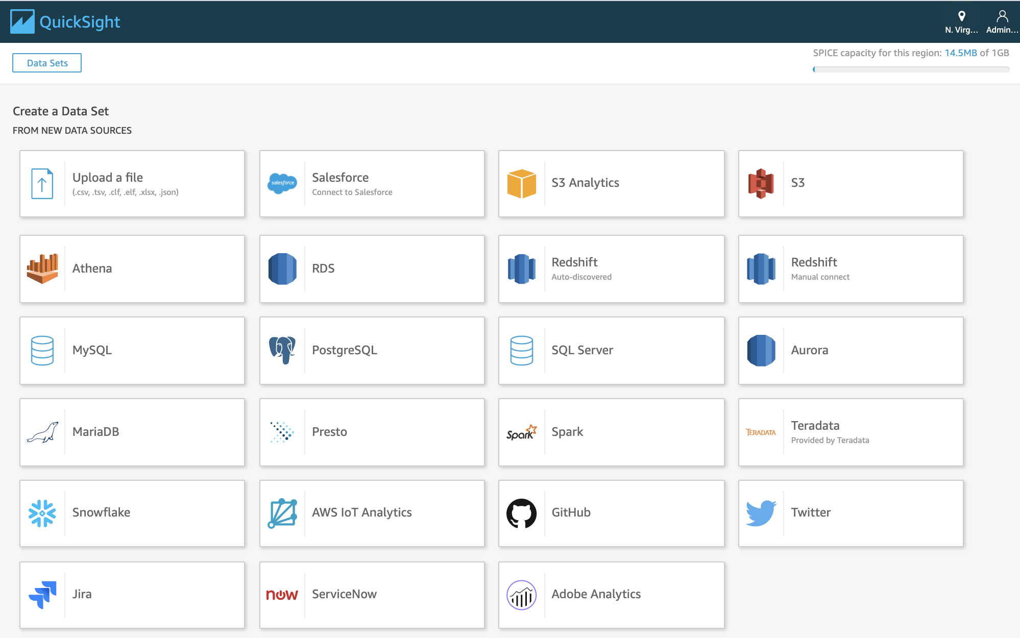
Figure 2-13. Amazon QuickSight > Supported Data Sources.
Here is the high-level QuickSight Workflow overview shown in Figure 2-14.
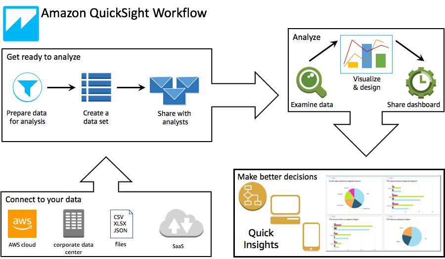
Figure 2-14. High-Level QuickSight Workflow.
Let’s use Amazon QuickSight to create a dashboard with our Amazon Customer Reviews Dataset.
Setup the Datasource
To add our dataset,
-
Click on “Manage data” on the upper right corner as shown in Figure 2-15, and then on “New data set”.
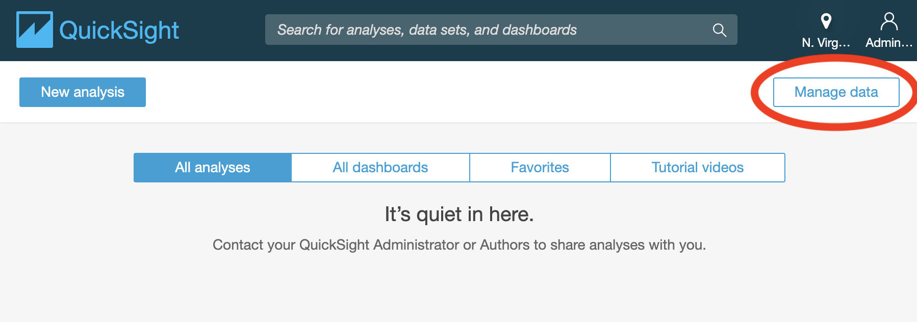
Figure 2-15. Amazon QuickSight > Manage data.
-
Click on “Athena” and provide a Data source name, for example amazon_reviews_parquet. Click on “Create data source”.
-
Select the previously generated dsoaws database from the drop-down list, and our amazon_reviews_parquet table. Click on “Select”.
-
Choose the “Directly query your data” option, and click on “Visualize”.
-
You should now see an empty graph and our dataset columns listed on the left as shown in Figure 2-16.

Figure 2-16. Amazon QuickSight after connecting our dataset
Query and Visualize the Dataset Within QuickSight
So let’s start visualizing.
-
Select a Horizontal chart bar graph under Visual types in the lower left corner as shown in Figure 4.17.
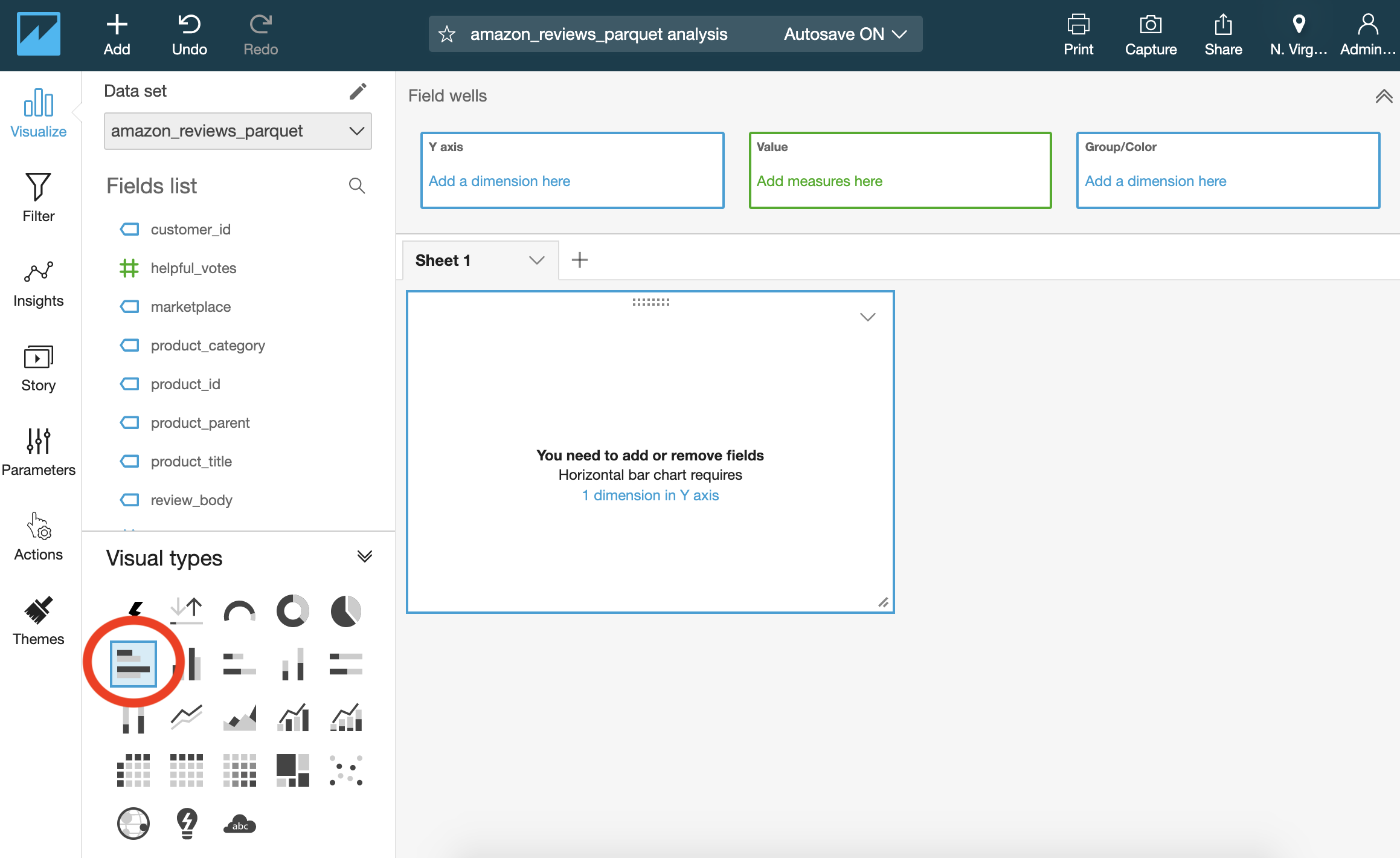
Figure 2-17. Amazon QuickSight, choose Horizontal bar chart.
-
Then drag the product_category field to the y-axis and value boxes. The visualization should now look like shown in Figure 2-18.
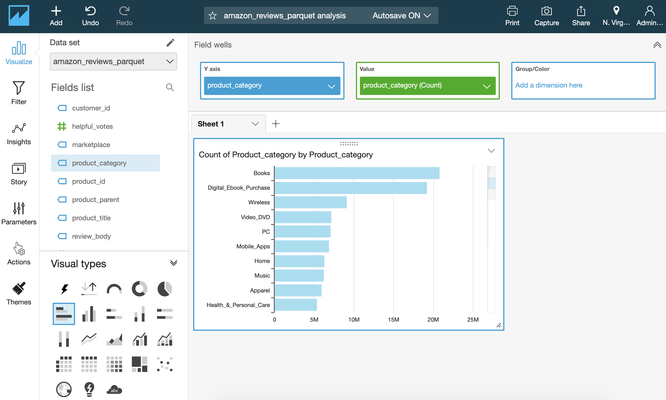
Figure 2-18. Amazon QuickSight, visualizing review counts per product category.
In just a few clicks, we have a visualization of review counts per product category - accessible by any device, anywhere.
Figure 2-19 shows how you can access the dashboard from a mobile device with the Amazon QuickSight Mobile App.

Figure 2-19. Using the Amazon QuickSight Mobile App to access dashboards.
Using this visualization, we quickly see the imbalance in our dataset, matching the results of our earlier Athena query. The two product categories of “Books” and “Digital_Ebook_Purchase” have by far the most reviews. We are going to address this in the next chapter where we prepare the data for model training.
Another important step in our early data exploration is to look for any data quality issues in our dataset. Let’s do this next.
Detect Data Quality Issues with Apache Spark
Data is never perfect - especially in a dataset with 130+ million rows spread across 20 years! Additionally, data quality may actually degrade over time as new application features are introduced and others are retired. Schemas evolve, code gets crusty, and queries get slow.
Since data quality is not always a priority for the upstream application teams, the downstream data engineering and data science teams need to handle bad or missing data. We want to make sure that our data is high quality for our downstream consumers including Business Intelligence, ML Engineering, and Data Science teams.
Figure 2-20 shows how applications generate data for engineers, scientists and analysts to consume, and which tools and services the various teams are likely to interact with to access that data.
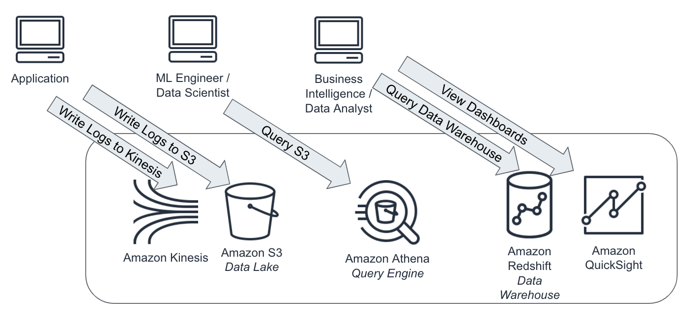
Figure 2-20. Applications generate data for engineers, scientists and analysts to consume.
Data quality can halt a data processing pipeline in its tracks. If these issues are not caught early, they can lead to misleading reports (ie. double-counted revenue), biased AI/ML models (skewed towards/against a single gender or race), and other unintended data products.
To catch these data issues early, we use Deequ, an open source library from Amazon that uses Apache Spark to analyze data quality, detect anomalies, and even “notify the Data Scientist at 3am” about a data issue. Deequ continuously analyzes data throughout the complete, end-to-end lifetime of the model from feature engineering to model training to model serving in production.
You can see a high-level overview of the Deequ architecture and components in Figure 2-21 below.

Figure 2-21. Overview of Deequ components: constraints, metrics, and suggestions.
Learning from run to run, Deequ will suggest new rules to apply during the next pass through the dataset. Deequ learns the baseline statistics of our dataset at model training time, for example - then detects anomalies as new data arrives for model prediction. This problem is classically called “training-serving skew”. Essentially, a model is trained with one set of learned constraints, then the model sees new data that does not fit those existing constraints. This is a sign that the data has shifted - or skewed - from the original distribution.
Since we have 130+ million reviews, we need to run Deequ on a cluster vs. inside our notebook. This is the trade-off of working with data at scale. Notebooks work fine for exploratory analytics on small data sets, but not suitable to process large data sets or train large models. We will use a notebook to kick off a Deequ Spark job on a cluster using SageMaker Processing Jobs.
SageMaker Processing Jobs
Processing Jobs as shown in Figure 2-22 can run any Python script - or custom Docker image - on the fully managed, pay-as-you-go AWS infrastructure using familiar open source tools such as Scikit-Learn and Apache Spark.
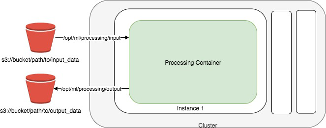
Figure 2-22. Container for a Processing Job.
Fortunately, Deequ is a high-level API on top of Apache Spark, so we use Processing Jobs to run our large-scale analysis job.
Note
Deequ is similar to TensorFlow Extended (TFX) in concept - specifically, the TensorFlow Data Validation TFDV) component. However, Deequ builds upon popular open source Apache Spark to increase usability, debug-ability, and scalability. Additionally, Apache Spark and Deequ natively support the Parquet format - our preferred file format for analytics.
Analyze Our Dataset with Deequ and Apache Spark
Table 4-1 shows just a few of the metrics that Deequ supports:
| Metric | Description | Usage Example |
| ApproxCountDistinct | Approximate number of distinct values using HLL++ | ApproxCountDistinct(“review_id”) |
| ApproxQuantiles | Approximate quantiles of a distribution. | ApproxQuantiles(“star_rating”, quantiles = Seq(0.1, 0.5, 0.9)) |
| Completeness | Fraction of non-null values in a column. | Completeness(“review_id”) |
| Compliance | Fraction of rows that comply with the given column constraint. | Compliance(“top star_rating”, “star_rating >= 4.0”) |
| Correlation | Pearson correlation coefficient | Correlation(“total_votes”, “star_rating”) |
| Maximum | Maximum value. | Maximum(“star_rating”) |
| Mean | Mean value; null values are excluded. | Mean(“star_rating”) |
| Minimum | Minimum value. | Minimum(“star_rating”) |
| MutualInformation | How much information about one column can be inferred from another column | MutualInformation(Seq(“total_votes”, “star_rating”)) |
| Size | Number of rows in a DataFrame. | Size() |
| Sum | Sum of all values of a column. | Sum(“total_votes”) |
| Uniqueness | Fraction of unique values | Uniqueness(“review_id”) |
Table 4-1. Sample Deequ metrics.
Let’s kick off the Apache Spark-based Deequ analyzer job by invoking the ScriptProcessor and launching a 10-node Apache Spark Cluster right from our notebook. Note: We need to build and push a custom Docker image with Apache Spark installed. This is the image_uri variable in this code sample. See the GitHub repository for more details on building this Docker image.
from sagemaker.processing import ScriptProcessor
processor =
	ScriptProcessor(base_job_name='SparkAmazonReviewsAnalyzer',
                   image_uri=image_uri,
                   command=['/opt/program/submit'],
                   role=role,
                   instance_count=10,
                   instance_type='ml.r5.8xlarge',
                   max_runtime_in_seconds=600,
                   env={
                       'mode': 'jar',
                       'main_class': 'Main'
                   })
processor.run(code='preprocess-deequ.py',
              arguments=['s3_input_data',
						 s3_input_data,
                         'S3_output_analyze_data',
						 s3_output_analyze_data,
              ]
)
Note
The code above calls a simple Python script that invokes the Apache Spark Scala code. Native PySpark is coming soon for Deequ to avoid this shim.
Below is our Deequ code specifying the various constraints we wish to apply to our TSV dataset. We are using TSV in this example to maintain consistency with the rest of the examples, but we could easily switch to Parquet with just a 1 line code change.
  val dataset = spark.read.option("sep", "	")
                        .option("header", "true")
                        .option("quote", "")
                        .schema(schema)
                        .csv("s3://amazon-reviews-pds/tsv")
Define the analyzers
  .addAnalyzer(Size())
  .addAnalyzer(Completeness("review_id"))
  .addAnalyzer(ApproxCountDistinct("review_id"))
  .addAnalyzer(Mean("star_rating"))
  .addAnalyzer(Compliance("top star_rating", "star_rating >= 4.0"))
  .addAnalyzer(Correlation("total_votes", "star_rating"))
  .addAnalyzer(Correlation("total_votes", "helpful_votes"))
Define the checks, compute the metrics, and verify check conditions
  .addCheck(
    Check(CheckLevel.Error, "Review Check")
    .hasSize(_ >= 130000000) // at least 130 million rows
    .hasMin("star_rating", _ == 1.0) // min is 1.0
    .hasMax("star_rating", _ == 5.0) // max is 5.0
    .isComplete("review_id") // should never be NULL
    .isUnique("review_id") // should not contain duplicates
    .isComplete("marketplace") // should never be NULL
	.isContainedIn("marketplace", Array("US", "UK", "DE", "JP", "FR"))
    .isNonNegative("year")) // should not contain negative values
  )
We have defined our set of constraints and assertions to apply to our dataset. Let’s run the job and ensure that our data is what we expect.
Below in Table 4-2 are the results from our Deequ job summarizing the results of the constraints and checks that we specified:
| check_name | columns | value |
| ApproxCountDistinct | review_id | 149075190 |
| Compleness | review_id | 1.00 |
| Compliance | Marketplace contained in US,UK, DE,JP,FR | 1.00 |
| Compliance | top star_rating | 0.79 |
| Correlation | helpful_votes,total_votes | 0.99 |
| Correlation | total_votes,star_rating | -0.03 |
| Maximum | star_rating | 5.00 |
| Mean | star_rating | 4.20 |
| Minimum | star_rating | 1.00 |
| Size | * | 150962278 |
| Uniqueness | review_id | 1.00 |
We learned the following:
-
review_id has no missing values and approximately (within 2% accuracy) 149,075,190 unique values.
-
79% of reviews have a “top” star_rating of 4 or higher.
-
total_votes and star_rating are weakly correlated.
-
helpful_votes and total_votes are strongly correlated.
-
The average star_rating is 4.20.
-
The dataset contains exactly 150,962,278 reviews (1.27% different than ApproxCountDistinct).
Deequ also suggests useful constraints based on the current characteristics of our dataset. This is useful when we have new data entering the system that may differ statistically from the original dataset. In the real world, this is very common as new data is coming in all the time.
In Table 4-3 are the checks - and the accompanying Scala code - that Deequ suggests we add to detect anomalies as new data comes arrives into the system:
| column | check | deequ_code |
| customer_id | ‘customer_id’ has type Integral | .hasDataType(customer_id”, ConstrainableDataTypes.Integral)” |
| helpful_votes | ‘helpful_votes’ has no negative values | .isNonNegative(helpful_votes”)” |
| review_headline | ‘review_headline’ has less than 1% missing values | .hasCompleteness( eview_headline”, _ >= 0.99, Some("It should be above 0.99!”))” |
| product_category | ‘product_category’ has value range ‘Books', ‘Digital_Ebook_Purchase', ‘Wireless', ‘PC', ‘Home', ‘Apparel', ‘Health & Personal Care', ‘Beauty', ‘Video DVD', ‘Mobile_Apps', ‘Kitchen', ‘Toys', ‘Sports', ‘Music', ‘Shoes', ‘Digital_Video_Download', ‘Automotive', ‘Electronics', ‘Pet Products', ‘Office Products', ‘Home Improvement', ‘Lawn and Garden', ‘Grocery', ‘Outdoors', ‘Camera', ‘Video Games', ‘Jewelry', ‘Baby', ‘Tools', ‘Digital_Music_Purchase', ‘Watches', ‘Musical Instruments', ‘Furniture', ‘Home Entertainment', ‘Video', ‘Luggage', ‘Software', ‘Gift Card', ‘Digital_Video_Games', ‘Mobile_Electronics', ‘Digital_Software', ‘Major Appliances', ‘Personal_Care_Appliances’ | .isContainedIn(product_category”, Array("Books”, "Digital_Ebook_Purchase”, "Wireless”, "PC”, "Home”, "Apparel”, "Health & Personal Care”, "Beauty”, "Video DVD”, "Mobile_Apps”, "Kitchen”, "Toys”, "Sports”, "Music”, "Shoes”, "Digital_Video_Download”, "Automotive”, "Electronics”, "Pet Products”, "Office Products”, "Home Improvement”, "Lawn and Garden”, "Grocery”, "Outdoors”, "Camera”, "Video Games”, "Jewelry”, "Baby”, "Tools”, "Digital_Music_Purchase”, "Watches”, "Musical Instruments”, "Furniture”, "Home Entertainment”, "Video”, "Luggage”, "Software”, "Gift Card”, "Digital_Video_Games”, "Mobile_Electronics”, "Digital_Software”, "Major Appliances”, "Personal_Care_Appliances”))” |
| vine | ‘vine’ has value range ‘N’ for at least 99.0% of values | .isContainedIn(vine”, Array("N”), _ >= 0.99, Some("It should be above 0.99!”))” |
In addition to the Integral type and not-negative checks, Deequ also suggests that we constrain product_category to the 43 currently-known values including Books, Software, etc. Deequ also recognized that at least 99% of the vine values are N and < 1% of review_headline values are empty, so it recommends that we add checks for these conditions moving forward.
Increase Performance and Reduce Cost
In this section, we want to provide some tips & tricks to increase performance and reduce cost during data exploration. You can optimize expensive SQL COUNT queries across large datasets by using approximate counts. Leveraging Redshift AQUA you can reduce network I/O and increase query performance. And if you feel your QuickSight dashboards could benefit from a performance increase, have a look at QuickSight SPICE.
Approximate Counts with HyperLogLog
Counting is a big deal in analytics. We always need to count users (daily active users), orders, returns, support calls, etc. Maintaining super-fast counts in an ever-growing dataset can be a critical advantage over competitors.
Both Redshift and Athena support HyperLogLog (HLL), a type of “cardinality-estimation” or COUNT DISTINCT algorithm designed to provide highly accurate counts (<2% error) in a small fraction of the time (seconds) requiring a tiny fraction of the storage (1.2KB) to store 130+ million separate counts.
The way this works is that Redshift and Athena update a tiny HLL data structure when inserting new data into the database (think of a tiny hash table). The next time a count query arrives from a user, Redshift and Athena simply look up the value in the HLL data structure and quickly returns the value - without having to physically scan all the disks in the cluster to perform the count.
Note
Other forms of HLL include HyperLogLog++, Streaming HyperLogLog, and HLL-TailCut+ among others. Count-Min Sketch and Bloom Filters are similar algorithms for approximating counts and set membership, respectively.
Let’s compare the execution times of both SELECT APPROXIMATE COUNT() and SELECT COUNT() in Redshift as follows:
	%%time
df = pd.read_sql_query("""
SELECT APPROXIMATE COUNT(DISTINCT customer_id)
FROM {}.{}
GROUP BY product_category
""".format(redshift_schema, redshift_table_2015), engine)
	-------------
%%time
df = pd.read_sql_query("""
SELECT COUNT(DISTINCT customer_id)
FROM {}.{}
GROUP BY product_category
""".format(redshift_schema, redshift_table_2015), engine)
You should see outputs similar to this:
For the query which used APPROXIMATE COUNT():
CPU times: user 3.66 ms, sys: 3.88 ms, total: 7.55 ms
Wall time: 18.3 s
For the query which used COUNT():
CPU times: user 2.24 ms, sys: 973 µs, total: 3.21 ms
Wall time: 47.9 s
Note
Note that we run the APPROXIMATE COUNT first to factor out the performance boost of the query cache. The COUNT is much slower. If you re-run, both queries will be very fast due to the query cache.
We see that APPROXIMATE COUNT DISTINCT is 160% faster than regular COUNT DISTINCT in this case. The results were approximately 1.2% different - satisfying the <2% error guaranteed by HyperLogLog.
Note
Reminder that HyperLogLog is an approximation. Approximations may not be suitable for use cases that require exact numbers such as financial reporting, etc.
Dynamically Scale Your Data Warehouse with Redshift AQUA
Existing data warehouses move data from storage nodes to compute nodes during query execution. This requires high network I/O between the nodes - and reduces query performance.
Figure 2-23 below shows a traditional data warehouse architecture with shared, centralized storage.
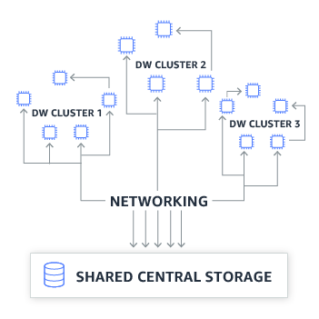
Figure 2-23. Traditional Data Warehouse with Shared, Centralized Storage.
Redshift Advanced Query Accelerator (AQUA) is a hardware-accelerated, distributed cache on top of your Redshift data warehouse. AQUA uses custom, AWS-designed chips to perform computations directly in the cache. This reduces the need to move data from storage nodes to compute nodes - and therefore reducing network I/O and increasing query performance. These AWS-designed chips are implemented in FPGAs and help speed up data encryption and compression for maximum security of your data. AQUA dynamically scales out more capacity, as well.
Figure 2-24 shows the AQUA architecture.

Figure 2-24. Redshift Advanced Query Accelerator (AQUA) Dynamically Scales Out As Needed.
Improve Dashboard Performance with QuickSight SPICE
Amazon QuickSight is built with the “Super-fast, Parallel, In-memory Calculation Engine” or SPICE. SPICE uses a combination of columnar storage, in-memory storage, and machine code generation to run low-latency queries on large datasets. Amazon QuickSight updates its cache as data changes in the underlying data sources including S3 and Redshift.
Summary
In this chapter, we answered various questions about our data using various tools from the AWS Analytics Stack including Athena and Redshift. We created a Business Intelligence (BI) dashboard using QuickSight and deployed a SageMaker Processing Job using Deequ and Apache Spark to continuously monitor data quality and detect anomalies as new data arrives into the system. This continuous monitoring creates confidence in our data pipelines - and allows downstream teams including Data Scientists and AI/ML Engineers to develop highly-accurate and relevant models for our applications to consume.
In the next chapter, we will engineer our dataset and prepare “features” to use in our model training, optimization, and deployment efforts going forward.