Chapter 6. Deploying Models to Production with SageMaker
In the previous chapters, you learned how to train and optimize models. In this chapter, we shift focus from model development in the research lab to model deployment in production. We demonstrate how to deploy, optimize, scale, and monitor models to serve our applications and business use cases. We will deploy our model as both a REST endpoint as well as a batch transformation job.
Collaborating with Multiple Teams
Model deployments require close collaboration between the application, data science, and devops teams to successfully productionize our models as shown in Figure 6-1.
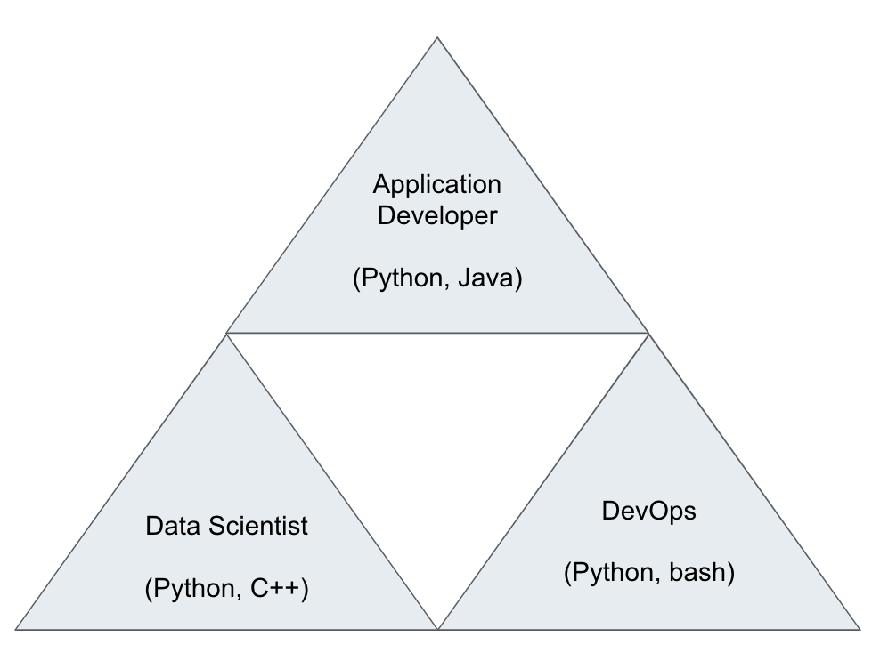
Figure 6-1. Productionizing machine learning applications requires collaboration between teams.
The data scientist delivers the trained model, the DevOps engineer provisions the needed infrastructure to host the model API, and the application developer integrates the model API calls into their applications. Each team must understand the needs and requirements of the other teams in order to implement an efficient workflow and smooth hand-off process.
Choose Level Of Customization
Similar to model training, you can choose between three(3) deployment options depending on the level of customization you desire as shown in Figure 6-2.
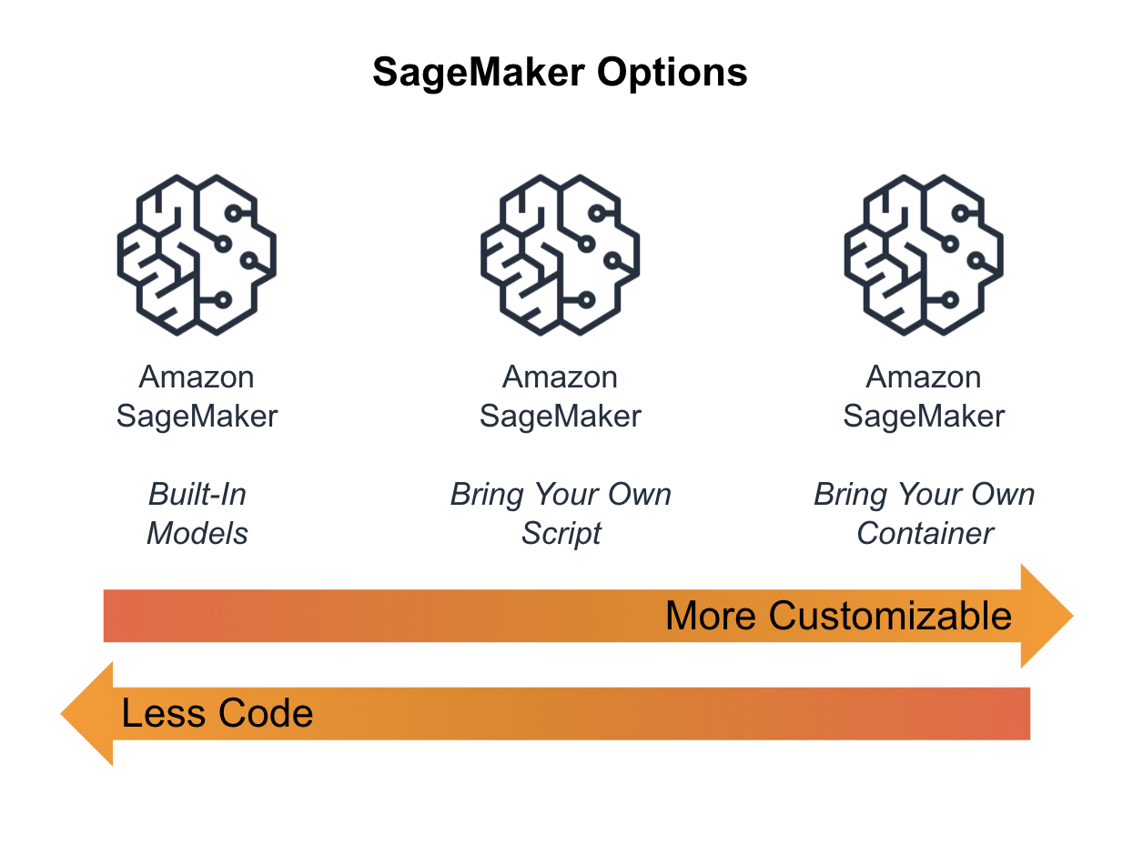
Figure 6-2. SageMaker Options to Deploy Your Model
Built-In Algorithms
Using a built-in SageMaker algorithm, you leverage both the pre-built inference code and model server container. These algorithms, shown in the table below, are targeted towards practitioners who don’t want to manage a lot of infrastructure and don’t need a lot of algorithm customizations.
| Classification Linear Learner XGBoost KNN |
Computer Vision Image Classification Object Detection Semantic Segmentation |
Working with Text BlazingText Supervised Unsupervised |
| Regression Linear Learner XGBoost KNN |
Anomaly Detection Random Cut Forests IP Insights |
Topic Modeling LDA NTM |
| Sequence Translation Seq2Seq |
Recommendation Factorization Machines |
Clustering KMeans |
| Feature Reduction PCA Object2Vec |
Forecasting DeepAR |
Bring Your Own Script
Similar to “bring your own script” or “script mode” for model training, SageMaker provides highly-optimized, open source inference containers for each of the familiar open source frameworks such as TensorFlow, PyTorch, MXNet, XGBoost, and Scikit-Learn as shown in Figure 4-3.

Figure 6-3. Popular AI and Machine Learning Frameworks
Script mode is a good balance of high customization and low maintenance, so we will choose this option for the examples in this chapter as shown in Figure 6-4.
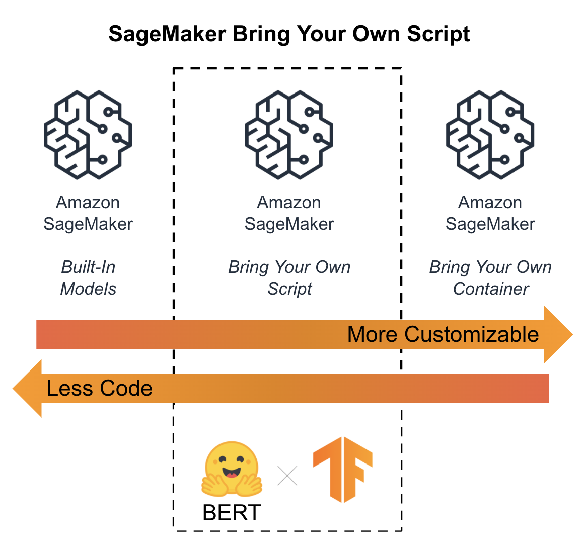
Figure 6-4. Script model with BERT and TensorFlow is a good balance of customization and maintenance
Bring Your Own Container
The most customizable inference option is to “bring your own container” (BYOC). This option lets you build and deploy your own inference container to SageMaker. This container can contain any library, framework, or model server. SageMaker will manage the low-level infrastructure for logging, monitoring, environment variables, S3 locations, etc. This option is targeted at systems-focused machine learning practitioners with custom inference needs.
Choose Real-Time or Batch Predictions
We need to understand the application and business context to choose between real-time and batch predictions. Are we trying to optimize for latency or throughput? Does the application require our models to scale automatically throughout the day to handle cyclic traffic requirements? Do we plan to compare models in production through A/B tests?
If our application requires low latency, then we should deploy the model as a real-time API to provide super-fast predictions on single prediction requests over HTTPS, for example. We can deploy, scale, and compare our model prediction servers with SageMaker Endpoints as shown in Figure 6-5.
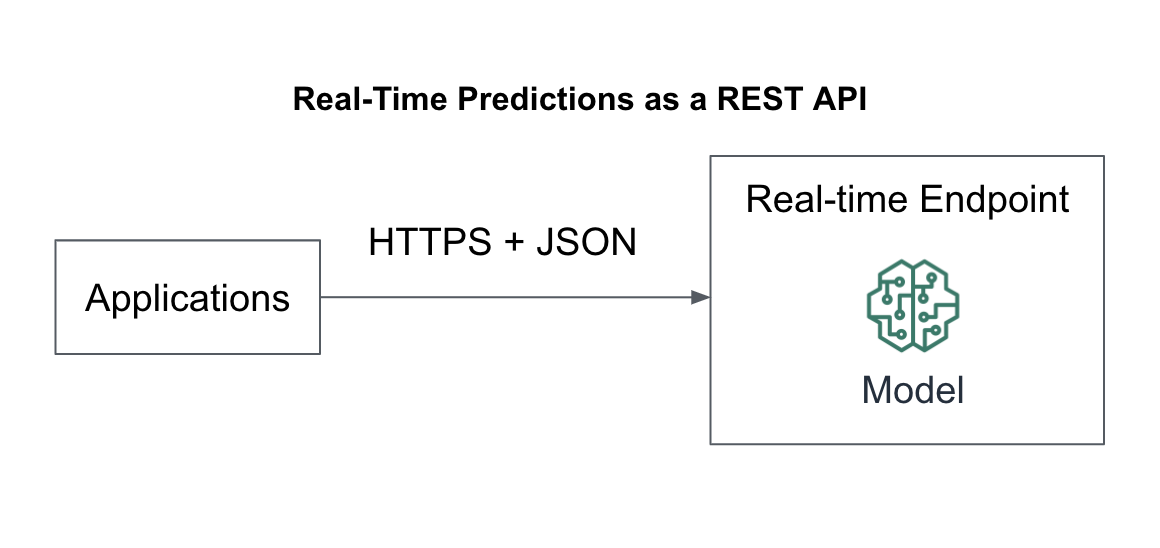
Figure 6-5. Real-time predictions as a REST API
For applications that require high throughput, we should deploy our model as a batch job to perform batch predictions on large amounts of data in S3, for example. We will use SageMaker Batch Transformations to perform the batch predictions along with a data store like RDS or DynamoDB to productionize the predictions as shown in Figure 6-6.

Figure 6-6. Batch predictions with SageMaker.
Real-Time Predictions with SageMaker Endpoints
In 2002, Jeff Bezos, CEO of Amazon, wrote a memo to his employees later called the “Bezos API Mandate”. The mandate dictated that all teams must expose their services through APIs - and communicate with each other through these APIs. This mandate addressed the “dead-lock” situation that Amazon faced back in the early 2000’s in which everybody wanted to build and use APIs, but nobody wanted to spend the time refactoring their monolithic code to support this idealistic best practice. The mandate released the deadlock and required all teams to build and use APIs within Amazon.
Note
Seen as the cornerstone of Amazon’s success early on, the Bezos API Mandate is the foundation of Amazon Web Services as we know it today. APIs helped Amazon re-use their internal ecosystem as scalable managed services for other organizations to build upon.
Following the Bezos API Mandate, we will deploy our model as a REST API using SageMaker Endpoints. SageMaker Endpoints are, by default, distributed containers. Applications invoke our models through a simple RESTful interface as shown in Figure 6-7 which shows the model deployed across multiple cluster instances and availability zones for higher availability.
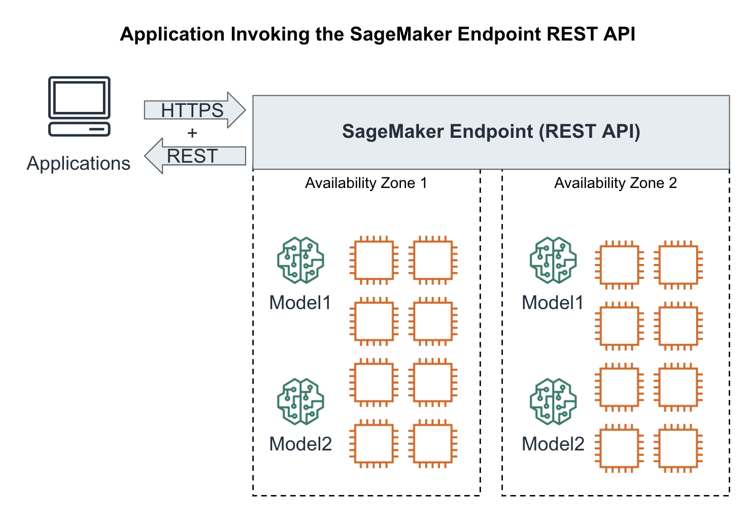
Figure 6-7. Application invoking our highly-available model as a REST endpoint
Deploy Model using SageMaker Python SDK
There are two ways to deploy the model using the SageMaker Python SDK. We can call deploy() on a model object, or we can call deploy() on a SageMaker estimator object that we used to train the model. Creating a model object also allows us to deploy a model that has been trained outside of the Amazon SageMaker platform.
Here is sample code for calling `deploy()` on a TensorFlow model:
from sagemaker.tensorflow.serving import Model
# Create the model object from a saved model
tf_model = Model(model_data=saved_model,
			role=role,
			framework_verison='2.1')
# Deploy the model
predictor = tf_model.deploy(initial_instance_count=1,
				instance_type = 'ml.m4.xlarge')
# Run a sample prediction
prediction = predictor.predict({'inputs': payload})
Endpoint Configuration
When we call deploy() SageMaker automatically creates a default EndpointConfig for the model endpoint. The EndpointConfig defines parameters such as whether to enable data capture for the model, the list of production variants and traffic split weights etc. We will see how to create a custom EndpointConfig in a later section.
Here is sample code for calling deploy() on a SageMaker estimator object after the training has completed:
from sagemaker.tensorflow.serving import TensorFlow# Create the estimatorestimator =TensorFlow(entry_point='train.py',role=role,train_instance_count=2,train_instance_type='ml.p3.2xlarge',framework_verison='2.1',py_version='py3')# Train the modelestimator.fit(training_data_uri)# Deploy the model from the estimatorpredictor = estimator.deploy(initial_instance_count=1,instance_type='ml.m4.xlarge')# Run a sample predictionprediction = predictor.predict({'inputs': payload})
Note that in both scenarios we can simply call predict() on the deployed model to run sample predictions. Coming back to our fine-tuned BERT model, let’s choose the first option to deploy the model into production:
from sagemaker.tensorflow.serving import Modelmodel =Model(model_data='s3://{}/{}/output/model.tar.gz'.format(bucket,training_job_name),role=role,framework_version='2.1.0')deployed_model = model.deploy(initial_instance_count=1,instance_type='ml.m4.xlarge',wait=False)endpoint_name = deployed_model.endpoint
Track Model Deployment in our Experiment
We also want to track the deployment within our experiment for data lineage.
from smexperiments.trial import Trialtrial = Trial.load(trial_name=trial_name)from smexperiments.tracker import Trackertracker_deploy = Tracker.create(display_name='deploy',sagemaker_boto_client=sm)deploy_trial_component_name = tracker_deploy.trial_component.trial_component_name# Attach the 'deploy' Trial Component and Tracker to the Trialtrial.add_trial_component(tracker_deploy.trial_component)# Track the Endpoint Nametracker_deploy.log_parameters({'endpoint_name': endpoint_name,})# Must save after loggingtracker_deploy.trial_component.save()
Analyze Model Deployment Lineage
Let’s use the Experiment Analytics to show us model lineage information:
from sagemaker.analytics import ExperimentAnalyticslineage_table = ExperimentAnalytics(sagemaker_session=sess,experiment_name=experiment_name,metric_names=['validation:accuracy'],sort_by="CreationTime",sort_order="Ascending",)lineage_df = lineage_table.dataframe()print(lineage_df)
If we print lineage_df the output should look similar to this (shortened):
| TrialComponentName | DisplayName | max_seq_/ length | test_split_/ percentage | train_split_/ percentage | validation_/ split_/ percentage | endpoint_/ name | SourceArn | |
|---|---|---|---|---|---|---|---|---|
| 0 | TrialComponent- 2020-06-06- ... | prepare | 128.0 | 0.05 | 0.9 | 0.05 | NaN | NaN |
| 1 | tensorflow-training- 2020-06-06- ... | train | 128.0 | NaN | NaN | NaN | NaN | arn:aws:sagemaker: us-east-1: ... |
| 2 | TrialComponent- 2020-06-06- ... | deploy | NaN | NaN | NaN | NaN | tensorflow-training- 2020-06-06- ... | NaN |
Invoking Predictions using the SageMaker Python SDK
Here is some simple application code to query our deployed endpoint for predictions. We define a RequestHandler class which transforms the raw prediction input data (our customer reviews text) into BERT tokens required by the model.
classRequestHandler(object):import jsondef __init__(self, tokenizer, max_seq_length):self.tokenizer = tokenizerself.max_seq_length = max_seq_lengthdef __call__(self, instances):transformed_instances = []for instance in instances:encode_plus_tokens = tokenizer.encode_plus(instance,pad_to_max_length=True,max_length=self.max_seq_length)input_ids = encode_plus_tokens['input_ids']input_mask = encode_plus_tokens['attention_mask']segment_ids = [0] * self.max_seq_lengthtransformed_instance = {"input_ids": input_ids,"input_mask": input_mask,"segment_ids": segment_ids}transformed_instances.append(transformed_instance)transformed_data = {"instances": transformed_instances}return json.dumps(transformed_data)
Similarly, we implement a ResponseHandler class which transforms the BERT model output into star rating classes.
classResponseHandler(object):import jsonimport tensorflow as tfdef __init__(self, classes):self.classes = classesdef __call__(self, response, accept_header):import tensorflow as tfresponse_body = response.read().decode('utf-8')response_json = json.loads(response_body)log_probabilities = response_json["predictions"]predicted_classes = []# Convert log_probabilities => softmax (all probabilities add up to 1) => argmax (final prediction)for log_probability in log_probabilities:softmax = tf.nn.softmax(log_probability)predicted_class_idx = tf.argmax(softmax, axis=-1, output_type=tf.int32)predicted_class = self.classes[predicted_class_idx]predicted_classes.append(predicted_class)return predicted_classes
The SageMaker Predictor class conveniently offers us a serializer and deserializer input parameter which we can use to pass our RequestHandler and ResponseHandler objects. The final prediction query looks like this:
import jsonfrom sagemaker.tensorflow.serving import Predictorfrom transformers import DistilBertTokenizertokenizer = DistilBertTokenizer.from_pretrained('distilbert-base-uncased')request_handler =RequestHandler(tokenizer=tokenizer,max_seq_length=128)response_handler =ResponseHandler(classes=[1, 2, 3, 4, 5])predictor =Predictor(endpoint_name=endpoint_name,sagemaker_session=sess,serializer=request_handler,deserializer=response_handler,content_type='application/json',model_name='saved_model',model_version=0)
Now, let’s test our model endpoint with two sample reviews:
import tensorflow as tfimport jsonreviews= ["This is great!","The worst product."]predicted_classes = predictor.predict(reviews)for predicted_class, review in zip(predicted_classes, reviews):print('[Predicted Star Rating: {}]'.format(predicted_class), review)
The output should look similar to this:
[Predicted Star Rating: 5] This is great![Predicted Star Rating: 1] The worst product.
Invoke Predictions from Using HTTP POST
In this example, we invoked the model endpoint directly using the Python SDK. When you productionize your machine learning applications you need to decide how to make your runtime inference endpoints available to client applications. You can call the SageMaker model endpoint API directly following this HTTP request/response syntax:
Request syntax:POST /endpoints/<EndpointName>/invocations HTTP/1.1Content-Type:ContentTypeAccept:AcceptX-Amzn-SageMaker-Custom-Attributes:<CustomAttributes>X-Amzn-SageMaker-Target-Model:<TargetModel> BodyResponse syntax:HTTP/1.1 200Content-Type:ContentTypex-Amzn-Invoked-Production-Variant:<InvokedProductionVariant>X-Amzn-SageMaker-Custom-Attributes:<CustomAttributes> Body
In this example, we implemented the data pre- and post-processing in our client application. The RequestHandler transformed our input review text into BERT tokens, and the ResponseHandler transformed the BERT model’s output into star rating classes. If you prefer to implement the pre- and post-processing steps server-side, you either include them in train.py as input_handler() and output_handler() functions. For more complex request and response handlers, you can deploy each step in their own container using SageMaker Inference Pipelines.
Creating Inference Pipelines
An inference pipeline is a sequence of containers deployed on a single endpoint. Following our example, we could deploy the RequestHandler as its own model in a separate Scikit-Learn container(Model 1), followed by the TensorFlow/BERT model in its own TensorFlow Serving container (Model 2), and succeeded by the ResponseHandler as its own model in a separate Scikit-Learn container (Model 3) as shown in Figure 6-8.
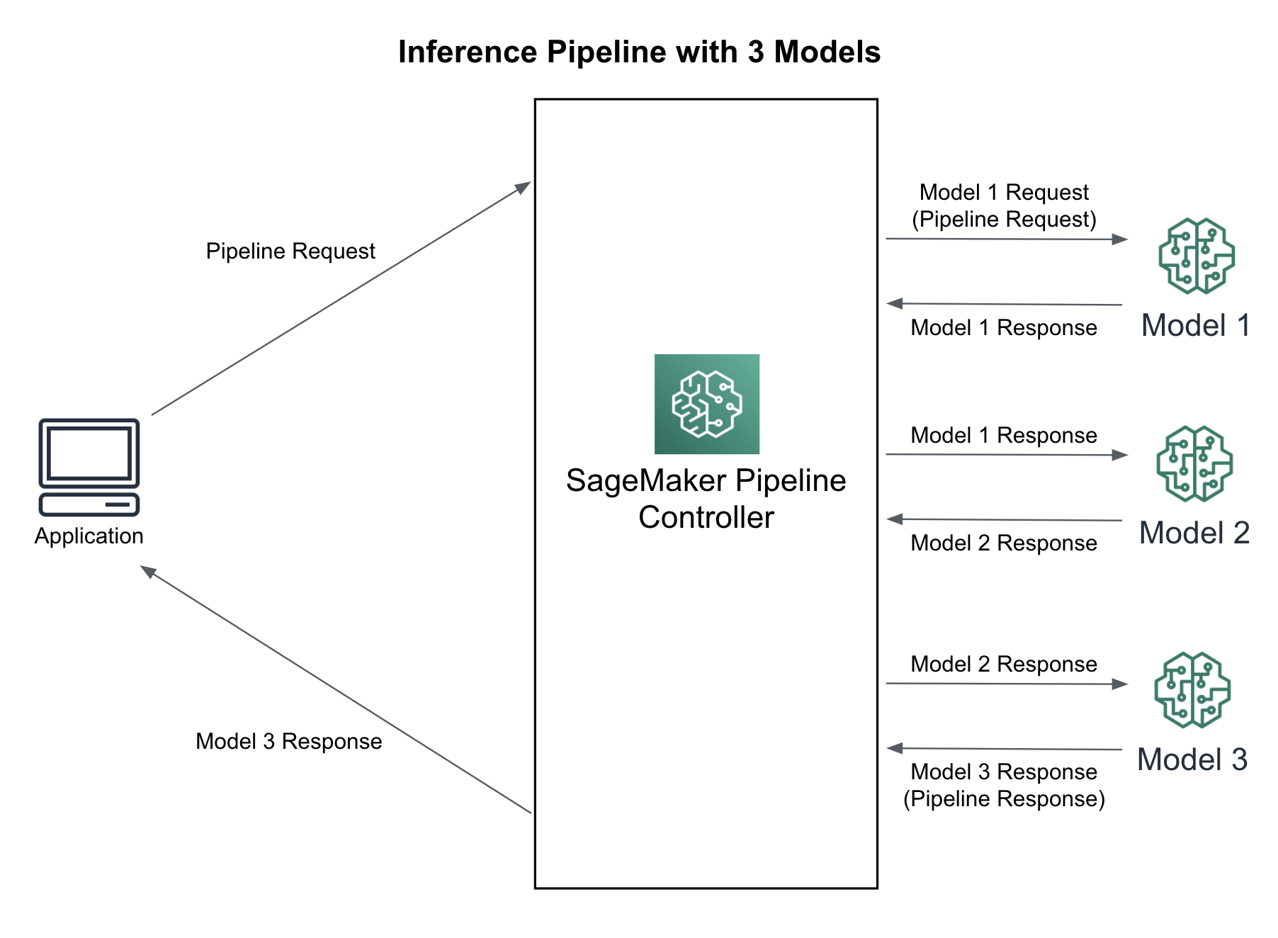
Figure 6-8. Inference Pipeline with Three(3) Models
You can also deploy completely unique models across different AI and machine learning frameworks including TensorFlow, PyTorch, Scikit-Learn, Apache Spark ML, etc. The model invocations are handled as a sequence of HTTPS requests between the containers controlled by SageMaker. One model’s response is used as the prediction request for the next model and so on. The last model returns the final response back to the SageMaker controller which returns the response back to the calling application. The inference pipeline is fully-managed by SageMaker and can be used for real-time predictions as well as batch transforms.
To deploy an inference pipeline, we need to create a PipelineModel comprising a list of model objects which represent the sequence of containers. We can then call deploy() on the PipelineModel which deploys the inference pipeline and returns the endpoint API:
# Define model name and endpoint namemodel_name = 'inference-pipeline-model'endpoint_name = 'inference-pipeline-endpoint'# Create a PipelineModel with a list of models to deploy in sequencepipeline_model =PipelineModel(name=model_name,role=sagemaker_role, models=[model1, model2, model3])# Deploy the PipelineModelpipeline_model.deploy(initial_instance_count=1,instance_type='ml.c5.xlarge', endpoint_name=endpoint_name)
The pipeline_model.deploy() returns a predictor as seen in the single model example. Whenever you make an inference request to this predictor, make sure you pass the data that the first model container expects. The predictor returns the output from the last model container..
If you want to run batch transform job with the pipeline model, just follow the steps of creating pipeline_model.transformer() object and call transform():
transformer = pipeline_model.transformer(instance_type='ml.c5.xlarge',instance_count=1,strategy='MultiRecord',max_payload=6,max_concurrent_transforms=8,accept='text/csv',assemble_with='Line',output_path='s3://my_bucket/path/')transformer.transform(data='s3://my_bucket/path/to/my/csv/data',content_type='text/csv',split_type='Line')
Deploying New Models
You can test and deploy new models behind a single SageMaker Endpoint with a concept called “production variants.” These variants can differ by hardware (CPU/GPU), by data (comedy/drama movies), or by region (US West or Germany North). You can shift traffic between the models in your endpoint for canary rollouts, blue/green deployments, A/B tests and multi-armed bandit (MAB) tests.
Split Traffic for Canary Rollouts
Since our data is continuously changing, our models need to evolve to capture this change. When we update our models, we may choose to do this slowly using a “canary rollout” named after an antiquated and morbid process of using a canary to early-detect if a human could breathe in a coal mine. If the canary survives the coal mine, then the conditions are good and we can proceed. If the canary does not survive, then we should make adjustments and try again later with a different canary. Similarly, we can point a small percentage of traffic to our “canary” model and test if the model services. Perhaps there is a memory leak or other production-specific issue that we didn’t catch in the research lab.
The combination of the cloud instance providing compute, memory and storage, and the model container application is called a “production variant.” The production variant defines the instance type, instance count, and model. By default, the SageMaker endpoint is configured with a single production variant, but you can add multiple variants as needed.
Here is the code to setup a single variant, VariantA, at a single endpoint receiving 100% of the traffic across 20 instances:
endpoint_config = sm.create_endpoint_config(EndpointConfigName='my_endpoint_config_name',ProductionVariants=[{'VariantName':'VariantA','ModelName': 'ModelA','InstanceType':'ml.m5.large','InitialInstanceCount':20,'InitialVariantWeight':100,}])
After creating a new production variant for our canary, we can create a new endpoint and point a small amount of traffic (5%) to the canary and point the rest of the traffic (95%) our existing variant as shown in Figure 6-9.

Figure 6-9. Splitting 5% traffic to a new model for a canary rollout
Below is the code to create a new endpoint including the new canary VariantB accepting 5% of the traffic to the canary. Note that we only specify 'InitialInstanceCount': 1 for the new canary, VariantB. Assuming 20 instance handles 100% of the traffic, then 1 instance can handle 5%.
updated_endpoint_config=[{'VariantName': 'VariantA','ModelName': 'ModelA','InstanceType':'ml.m5.large','InitialInstanceCount': 20,'InitialVariantWeight': 95,},{'VariantName': 'VariantB','ModelName': 'ModelB','InstanceType':'ml.m5.large','InitialInstanceCount':1,'InitialVariantWeight':5,}])sm.update_endpoint(EndpointName='my_endpoint_name',EndpointConfigName='my_endpoint_config_name')
Canary rollouts release new models safely to a small percentage of users for initial production testing in the wild. They are useful if you want to test in live production without affecting the entire user base. Since the majority of traffic goes to the existing model, the cluster size of the canary model can be relatively small since it’s only receiving 5% traffic. In the example above, we are only using a single instance for the canary variant.
Shift Traffic for Blue/Green Deployments
If the new model performs well, we can process with a blue/green deployment to shift all traffic to the new model as shown in Figure 6-10. Blue/green deployments help to reduce downtime in the case of failure. You spin up a full copy of the existing cluster using the canary model instead of the existing model. You then shift all the traffic from the old cluster (blue) over to the new cluster (green).
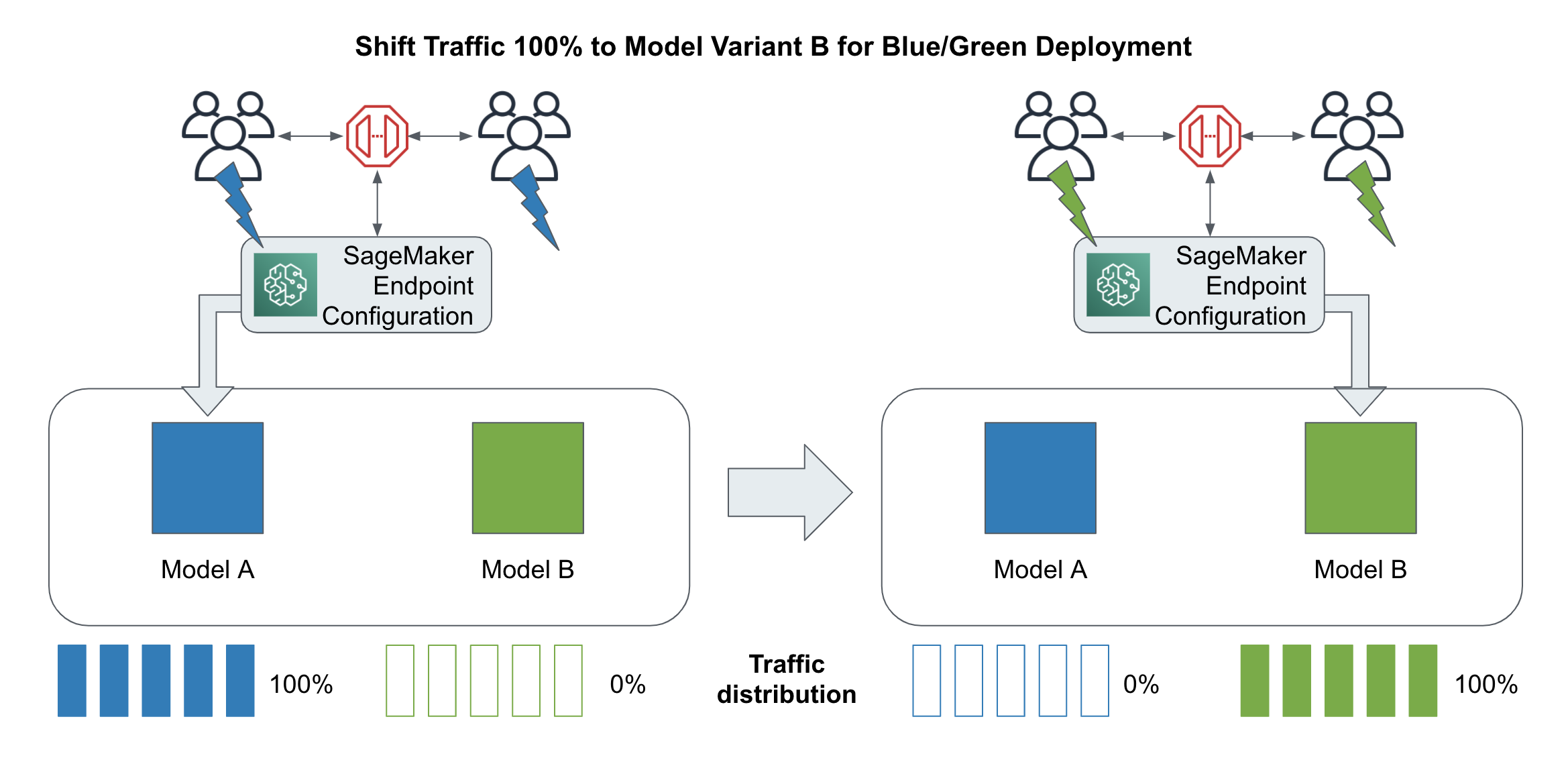
Figure 6-10. Shift traffic for blue/green deployments.
Below is the code to update our endpoint and shift 100% of the traffic to the successful canary model, VariantB. Note that we have also increased the size of the new cluster to match the existing cluster since the new cluster is now handling all of the traffic.
updated_endpoint_config=[{'VariantName': 'VariantA','ModelName': 'ModelA','InstanceType':'ml.m5.large','InitialInstanceCount': 20,'InitialVariantWeight': 0,},{'VariantName': 'VariantB','ModelName': 'ModelB','InstanceType':'ml.m5.large','InitialInstanceCount':20,'InitialVariantWeight': 100,}])sm.update_endpoint_weights_and_capacities(EndpointName='my_endpoint_name',DesiredWeightsAndCapacities=updated_endpoint_config)
We will keeping the old cluster with VariantA idle for 24 hours, let’s say, in case our canary fails unexpectedly and we need to rollback quickly to the old cluster. After 24 hours, we can remove the old environment and complete the blue/green deployment. Below is the code to remove the old model, VariantA, by removing VariantA from the endpoint configuration and updating the endpoint.
updated_endpoint_config=[{'VariantName': 'VariantB','ModelName': 'ModelB','InstanceType':'ml.m5.large','InitialInstanceCount': 2,'InitialVariantWeight': 100,}])sm.update_endpoint(EndpointName='my_endpoint_name',EndpointConfigName='my_endpoint_config_name')
While keeping the old cluster idle for a period of time - 24 hours, in our example - may seem wasteful, consider the cost of an outage during the time needed to rollback and scale out the previous model, VariantA. Sometimes the new model cluster works fine for the first few hours, then degrades or crashes unexpectedly after a night-time cron job, early-morning product catalog refresh, or other untested scenario. In these cases, we were able to immediately switch traffic back to the old cluster and conduct business as usual.
Testing and Comparing New Models
We can test new models behind a single SageMaker Endpoint using the same “production variant” concept described in the previous section on model deployment. In this section, we will configure our SageMaker Endpoint to shift traffic between the models in your endpoint to compare model performance in production using A/B and multi-armed bandit (MAB) tests.
When testing our models in production, we need to define and track the business metrics that we wish to optimize. The business metric is usually tied to revenue or user engagement such as orders purchased, movies watched, or ads clicked. We can store the metrics in any database such as DynamoDB as shown in Figure 6-11. Analysts and scientists will use this data to determine the winning model from our tests.

Figure 6-11. : Tracking business metrics to determine the best model variant
Continuing with our text-classifier example, we will create a test to maximize the number of successfully-labeled customer service messages. As customer service receives new messages, our application will predict the message’s star_rating (1-5) and route 1’s and 2’s to a high-priority customer service queue. If the representative agrees with the predicted star_rating, they will mark our prediction as successful (positive feedback), otherwise they will mark the prediction as unsuccessful (negative feedback.) Unsuccessful predictions will be routed to a human-in-the-loop workflow using Amazon Augmented AI and SageMaker Ground Truth as shown in the Augmented AI chapter. We will then choose the model variant with the most successful number of star_rating predictions - and start shifting traffic to this winning variant. Let’s dive deeper into managing the experiments and shifting the traffic.
Perform A/B Tests to Compare Model Variants
Similar to canary rollouts, we can use traffic splitting to direct subsets of users to different model variants for the purpose of comparing and testing different models in live production. The goal is to see which variants perform better. Often, these tests need to run for a long period of time (weeks) to be statistically significant. Figure 6-12 shows 2 different recommendation models deployed using a random 50-50 traffic split between the 2 variants.
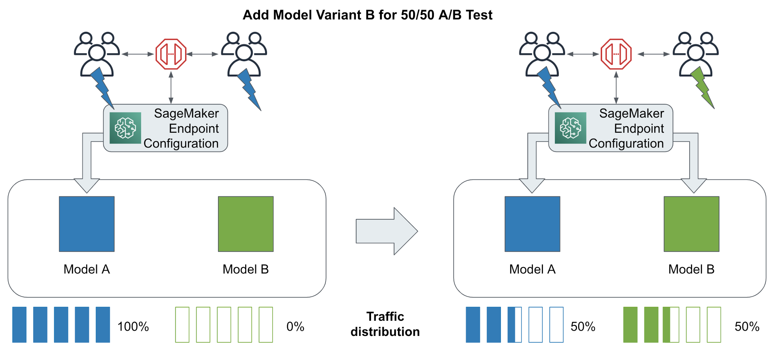
Figure 6-12. A/B Testing with two(2) model variants by splitting traffic 50-50
While A/B testing seems similar to canary rollouts, they are focused on gathering data about different variants of a model. A/B tests are targeted to larger user groups, take more traffic, and run for longer periods of time. Canary rollouts are focused more on risk mitigation and smooth upgrades.
One example for a model A/B test could be streaming music recommendations. Let’s assume we are recommending a playlist for Sunday mornings. You might want to test if you can identify specific user groups which are more likely to listen to powerful wake-up beats (model A) or that prefer smooth lounge music (model B). Let’s implement this A/B test using Python. We start with creating a SageMaker endpoint configuration which defines two production variants: one for model A, and one for model B. We initialize both production variants with the identical instance types and instance counts.
import timetimestamp = '{}'.format(int(time.time()))endpoint_config_name= '{}-{}'.format(training_job_name, timestamp)variantA = production_variant(model_name='ModelA',instance_type="ml.m5.large",initial_instance_count=1,variant_name='VariantA',initial_weight=50)variantB = production_variant(model_name='ModelB',instance_type="ml.m5.large",initial_instance_count=1,variant_name='VariantB',initial_weight=50)endpoint_config = sm.create_endpoint_config(EndpointConfigName=endpoint_config_name,ProductionVariants=[variantA, variantB])endpoint_name= '{}-{}'.format(training_job_name, timestamp)endpoint_response = sm.create_endpoint(EndpointName=endpoint_name,EndpointConfigName=endpoint_config_name)
After we have monitored the performance of both models for a period of time, we can shift 100% of the traffic to the better performing model, Model B in our case. Let’s shift our traffic from a 50/50 split to a 0/100 split as shown in Figure 6-13.

Figure 6-13. A/B testing traffic shift from 50/50 to 0/100.
Below is the code to shift all traffic to VariantB and ultimately remove VariantA we are confident that VariantB is working correctly.
updated_endpoint_config= [{'VariantName': 'VariantA','DesiredWeight':0,},{'VariantName': 'VariantB','DesiredWeight':100,}]sm.update_endpoint_weights_and_capacities(EndpointName='my_endpoint_name',DesiredWeightsAndCapacities=updated_endpoint_config)updated_endpoint_config=[{'VariantName': 'VariantB','ModelName': 'ModelB','InstanceType':'ml.m5.large','InitialInstanceCount': 2,'InitialVariantWeight': 100,}])sm.update_endpoint(EndpointName='my_endpoint_name',EndpointConfigName='my_endpoint_config_name')
Reinforcement Learning with Multi-Armed Bandit Testing
A/B tests must run for a period of time - sometimes weeks or months - before they are considered statistically significant. During this time, we may have deployed a bad model variant that is negatively affecting revenue. However, if we stop the test, we can’t rule out that the poor-performing model is caused merely by random chance.
A more dynamic method for testing different model variants is called Multi-Armed Bandits (MABs). Named after a slot machine which can quickly take your money, these mischievous bandits can actually earn you quite a bit of money by dynamically shifting traffic to the winning model variants much sooner than with an A/B test. This is the “exploit” part of the MAB. At the same time, the MAB continues to “explore” the non-winning model variants just in case the early winners were not the overall best model variants. This dynamic pull between “exploit and explore” are what give MABs their power.
Based on reinforcement learning, MAB’s rely on the feedback positive-negative mechanism described earlier in the A/B testing section. The MAB acts as the primary SageMaker Endpoint and dynamically shifts the prediction traffic as shown in Figure 6-14.
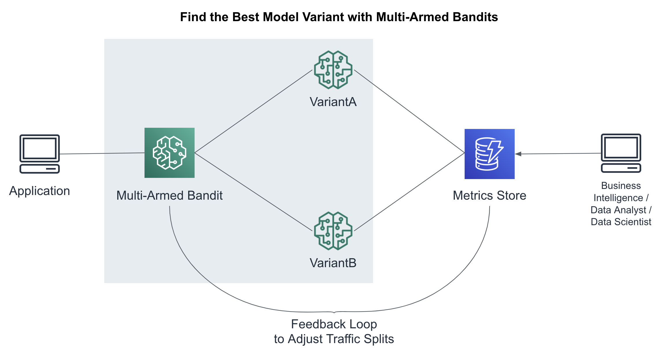
Figure 6-14. : Find the best model variant using multi-armed bandits
The multi-armed bandit chooses the model variant based on the current success metrics and the chosen exploit-explore strategy. There are two(2) popular MAB strategies: Epsilon Greedy and Thompson’s Sampling. Epsilon Greedy uses a fixed exploit-explore threshold while Thompson’s Sampling uses a more sophisticated and dynamic threshold based on prior information - a technique rooted in Bayesian statistics. The MAB is aware of the latest success metrics and will adjust the prediction traffic accordingly.
Auto-Scale SageMaker Endpoints using CloudWatch
While we can manually scale using the InstanceCount parameter in EndpointConfig, we can configure our endpoint to automatically scale out (more instances) or in (less instances) based on a given metric like requests per second. As more requests come in, SageMaker will automatically scale your model cluster to meet the demand.
In the cloud, we talk about “scaling in” and “scaling out” in addition to the typical “scaling down” and “scaling up.” Scaling in and out refers to removing and adding instances of the same type, respectively. Scaling down and up refers to using smaller or bigger instance types, respectively. Larger instances have more CPUs, GPUs, memory, and network bandwidth, typically.
It’s best to use homogenous instance types when defining your cluster. If we mix instance types, we may have difficulty tuning the cluster and defining scaling policies that apply consistently to every instance in the heterogeneous cluster. When trying new instance types, we recommend creating a new cluster with only that instance type and comparing each cluster as a single unit.
Define a Scaling Policy with Custom Metrics
Netflix is known to use a custom auto-scaling metric called “Starts per Second” or SPS. A start is recorded every time a user clicks “play” to watch a movie or tv show. This was a key metric for auto scaling as the more “Starts per Second”, the more traffic we would start receiving on our streaming control plane.
Assuming we are publishing the “StartsPerSecond” metric, we can use this custom metric to scale out our cluster as more movies are started. This metric is called a “target tracking” metric and we need to define the metric name, target value, model name, variant name, and summary statistic. The scaling policy below will begin scaling out the cluster if the aggregate StartsPerSecond metric exceeds an average of 50% across all instances in your model-serving cluster.
{  "TargetValue": 50,
  "CustomizedMetricSpecification":
  {
    "MetricName": "StartsPerSecond",
    "Namespace": "/aws/sagemaker/Endpoints",
    "Dimensions": [
      {"Name": "EndpointName", "Value": "ModelA" },
      {"Name": "VariantName","Value": "VariantA"}
    ],
    "Statistic": "Average",
    "Unit": "Percent"
  }
}
When using custom metrics for your scaling policy, you should pick a metric that measures instance utilization, decreases as more instances are added, and increases as instances are removed.
Using Pre-Defined Metrics
For our example, we will use an equivalent, pre-defined metric exposed by SageMaker Endpoints called “InvocationsPerInstance” as follows. The scaling policy below will begin scaling out the cluster if the aggregate InvocationsPerSecond metric exceeds an average of 60% across all instances in your model-serving cluster.
{  "TargetValue": 60.0,
  "PredefinedMetricSpecification":
  {
    "PredefinedMetricType":
"SageMakerVariantInvocationsPerInstance"
  }
}
Tuning Responsiveness Using a Cool Down Period
When your endpoint is autoscaling in or out, you likely want to specify a “cool down” period in seconds. A cool down period essentially reduces the responsiveness of the scaling policy by defining the number of seconds between iterations of the scale events. While you likely want to scale out quickly when a spike of traffic comes in, you may want to slowly scale in to make sure you’re handling any temporary dips in traffic during these scale out events. The following scaling policy will take twice as long to scale in as it does to scale out as shown in the ScaleInColldown and ScaleOutCooldown attributes below.
{
  "TargetValue": 60.0,
  "PredefinedMetricSpecification":
  {
    "PredefinedMetricType":
"SageMakerVariantInvocationsPerInstance"
  },
  "ScaleInCooldown": 600,
  "ScaleOutCooldown": 300}
Monitor Predictions and Detect Drift
The world continues to change around us. Customer behavior changes relatively quickly. The application team is releasing new features. The Netflix catalog is swelling with new content. Fraudsters are finding clever ways to hack our credit cards. A continuously-changing world requires continuously-changing predictive models that can detect and capture this “drift” and trigger a re-train to increase model performance. By automatically recording SageMaker Endpoint predictions (and their inputs), SageMaker Model Monitor automatically detects and measures this drift. Model Monitor will notify you when the drift reaches a certain threshold from a baseline specified during model deployment.
To enable Model Monitor, we need to perform the following steps:
- Enable Data Capture
-
Enable the endpoint to capture data from incoming inference requests to a trained model and the resulting model predictions.
- Create a Baseline
-
Create a baseline from the dataset that was used to train the model. Model monitor uses AWS Deequ Open Source to identify the baseline schema constraints and statistics for each feature.
- Schedule Monitoring Jobs
-
Create a monitoring schedule specifying what data to collect, how often to collect it, how to analyze it, and which reports to produce.
- Interpret Results
-
Inspect the reports, which compare the latest data with the baseline, and check for any violations reported and for metrics and notifications from Amazon CloudWatch.
Let’s dive deeper into each of these steps to monitor our predictions in production.
Enable Data Capture
SagMaker Model Monitor analyzes your model predictions (and their inputs) to detect drift. So the first step to configuring Model Monitor is to enable data capture for a given endpoint as shown in Figure 6-15.
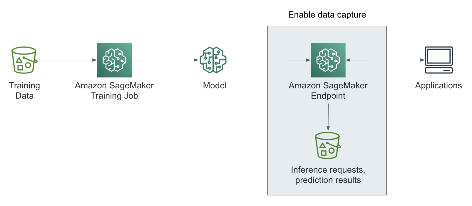
Figure 6-15. Enable model endpoint data capture.
Below is the code to enable data capture. You can define all configuration options in the DataCaptureConfig object. You can choose to capture the request payload, the response payload or both with this configuration. The capture config applies to all model production variants of the endpoint.
from sagemaker.model_monitor import DataCaptureConfigdata_capture_config =DataCaptureConfig(enable_capture=True,sampling_percentage=100,destination_s3_uri='s3://my_bucket/path/')Next, you pass theDataCaptureConfigin themodel.deploy()call:predictor = model.deploy(initial_instance_count=1,instance_type='ml.m4.xlarge',endpoint_name=endpoint_name,data_capture_config=data_capture_config)
We are now capturing all inference requests and prediction results in the specified S3 destination. In order to detect any model or data drift, we need to create a baseline to compare the data against.
{"captureData":{"endpointInput":{"observedContentType":"application/json","mode":"INPUT","data":"{"instances": [{"input_ids": [101, 2023, 2003, 2307, 999, 102, 0, 0, 0, 0, 0, 0, 0, 0, 0, 0, 0, 0, 0, 0, 0, 0, 0, 0, 0, 0, 0, 0, 0, 0, 0, 0, 0, 0, 0, 0], "input_mask": [1, 1, 1, 1, 1, 1, 0, 0, 0, 0, 0, 0, 0, 0, 0, 0, 0, 0, 0, 0, 0, 0, 0, 0, 0, 0, 0, 0, 0, 0, 0, 0, 0, 0, 0, 0], "segment_ids": [0, 0, 0, 0, 0, 0,0, 0, 0, 0, 0, 0, 0, 0, 0, 0, 0, 0, 0, 0, 0, 0, 0, 0, 0, 0, 0, 0, 0, 0, 0, 0, 0, 0, 0, 0]}, {"input_ids": [101, 2023, 2003, 6659, 1012, 102, 0, 0, 0, 0, 0, 0, 0, 0, 0, 0, 0, 0, 0, 0, 0, 0, 0, 0, 0, 0, 0, 0, 0, 0, 0, 0, 0, 0, 0, 0], "input_mask": [1, 1, 1, 1, 1, 1, 0, 0, 0, 0, 0, 0, 0], "segment_ids": [0, 0, 0, 0, 0, 0, 0, 0, 0, 0, 0, 0, 0]}]}","encoding":"JSON"},"endpointOutput":{"observedContentType": "application/json","mode":"OUTPUT","data":"{ "predictions":[[-1.5448699, -2.04928493, -1.71272779, 0.172660828, 4.16521502], [3.47782397, -0.372900903, -1.70296526, -1.61752951, -0.441117555] ]}","encoding":"JSON"}},"eventMetadata":{"eventId":"e2a31d52-5685-4105-9ee1-cc28d4be7c91","customAttributes":["tfs-model-name=saved_model"],"inferenceTime":"2020-05-17T03:18:26Z"},"eventVersion":"0"}
Create Baseline Statistics and Constraints for Features
A baseline helps us detect drift of input features relative to the features used to train the model. We typically use our training dataset to create the first baseline as shown in Figure 6-16.
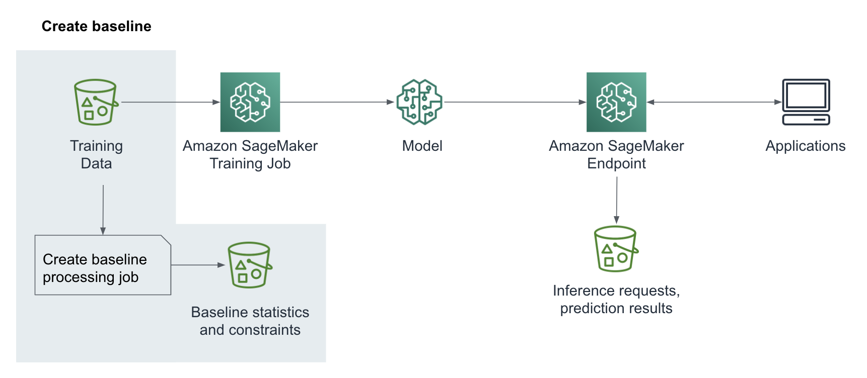
Figure 6-16. Create a baseline
The training dataset schema and the inference dataset schema must match exactly including the number of features and the order in which they are passed in for inference. We can now start a SageMaker ProcessingJob to suggest a set of baseline constraints and generate statistics of the data with
DefaultModelMonitor.suggest_baseline():from sagemaker.model_monitor import DefaultModelMonitorfrom sagemaker.model_monitor.dataset_format import DatasetFormatmy_default_monitor =DefaultModelMonitor(role=role,instance_count=1,instance_type='ml.m5.xlarge',volume_size_in_gb=20,max_runtime_in_seconds=3600,)my_default_monitor.suggest_baseline(baseline_dataset='s3://my_bucket/path/some.csv',dataset_format=DatasetFormat.csv(header=True),output_s3_uri='s3://my_bucket/output_path/',wait=True)
After the baseline job has finished, you can explore the generated statistics as follows:
import pandas as pdbaseline_job = my_default_monitor.latest_baselining_jobstatistics = pd.io.json.json_normalize(baseline_job.baseline_statistics().body_dict["features"])
Here is an example set of statistics for our `review_body` prediction inputs:
"name" : "Review Body","inferred_type" : "String","numerical_statistics" : {"common" : {"num_present" : 1420,"num_missing" : 0}, "data" : [ [ "I love this item.", "This item is OK", … ] ]
You can explore the generated constraints as follows:
constraints = pd.io.json.json_normalize(
baseline_job.suggested_constraints().body_dict["features"])
Here is an example of the constraints defined for our `review_body` prediction inputs:
{"name" : "Review Body","inferred_type" : "String","completeness" : 1.0}
Note
Under the hood, Model Monitor runs a SageMaker Processing Job on your behalf similar to the Processing Job that we used to analyze the statistics of the Amazon Customer Reviews Dataset.
We now have the foundation to schedule monitoring jobs that continuously check our real-time model performance against the created baseline.
Schedule Monitoring Jobs
SageMaker Model Monitor gives us the ability to continuously monitor the data collected from the endpoints on a schedule. You can create the schedule with the CreateMonitoringSchedule API defining a periodic interval. Similar to the baseline job, Model Monitor starts a SageMaker ProcessingJob which compares the dataset for the current analysis with the baseline statistics and constraints. The result is a violation report. In addition, Model Monitor sends metrics for each feature to Amazon CloudWatch as shown in Figure 9.17.

Figure 6-17. Schedule model monitoring jobs
You can create a model monitoring schedule for an endpoint with my_default_monitor.create_monitoring_schedule(). In the configuration of the monitoring schedule, you point to the baseline statistics and constraints and define a cron schedule.
from sagemaker.model_monitor import DefaultModelMonitorfrom sagemaker.model_monitor import CronExpressionGeneratormon_schedule_name = 'my-model-monitor-schedule'my_default_monitor.create_monitoring_schedule(monitor_schedule_name=mon_schedule_name,endpoint_input=predictor.endpoint,output_s3_uri=s3_report_path,statistics=my_default_monitor.baseline_statistics(),constraints=my_default_monitor.suggested_constraints(),schedule_cron_expression=CronExpressionGenerator.hourly(),enable_cloudwatch_metrics=True,)
Model Monitor now runs at the scheduled intervals and analyzes the captured data against the baseline. The job creates a violation report and stores the report in Amazon S3, along with a statistics report for the collected data.
Once the monitoring job has started its executions, you can use list_executions() to view them:
executions = my_monitor.list_executions()
You can also view the status of a specific execution, e.g. the latest monitoring job:
latest_execution = executions[-1]latest_execution.describe()['ProcessingJobStatus']latest_execution.describe()['ExitMessage']
The Model Monitor jobs should exit with one of the following status:
- Completed
-
This means the monitoring execution completed and no issues were found in the violations report.
- CompletedWithViolations
-
This means the execution completed, but constraint violations were detected.
- Failed
-
The monitoring execution failed, maybe due to client error (such as incorrect role permissions) or infrastructure issues.
- Stopped
-
The job exceeded the max runtime or was manually stopped. To troubleshoot further, you can check
FailureReasonandExitMessage.
Note
You can create your own custom monitoring schedules and procedures using preprocessing and postprocessing scripts. You can also build your own analysis container.
Interpret Results
With the monitoring data collected and continuously compared against the model baseline, we are now in a much better position to make decisions about how to improve the model. Depending on the model monitoring results, you might decide to retrain and redeploy the model. In this final step, we visualize and interpret the results as shown in Figure 6-18.

Figure 6-18. Interpret results.
Let’s query for the location for the generated reports.
report_uri=latest_execution.output.destinationprint('Report Uri: {}'.format(report_uri))
Next, we can list the generated reports:
from urllib.parse import urlparses3uri = urlparse(report_uri)report_bucket = s3uri.netlocreport_key = s3uri.path.lstrip('/')print('Report bucket: {}'.format(report_bucket))print('Report key: {}'.format(report_key))s3_client = boto3.Session().client('s3')result = s3_client.list_objects(Bucket=report_bucket,Prefix=report_key)report_files = [report_file.get("Key") for report_file inresult.get('Contents')]print("Found Report Files:")print(" ".join(report_files))
Output:
s3://<bucket>/<prefix>/constraint_violations.json
s3://<bucket>/<prefix>/constraints.json
s3://<bucket>/<prefix>/statistics.json
We already looked at constraints.json and statistics.json, so let’s analyze the violations:
violations =my_default_monitor.latest_monitoring_constraint_violations()violations = pd.io.json.json_normalize(violations.body_dict["violations"])
Here are example violations for our review_body inputs:
{"feature_name" : "Review Body","constraint_check_type" : "data_type_check","description" : "Value: 1.0 meets the constraint requirement"}, {"feature_name" : "Review Body","constraint_check_type" : "baseline_drift_check","description" : "Numerical distance: 0.2711598746081505 exceeds numerical threshold: 0"}
To find the root cause of this drift, we want to examine the prediction inputs and examine any upstream application bugs (or features) that may have been recently introduced. Perhaps the application team started to feature emojis as the primary review mechanism - and our language model was not trained on emojis. In this case, we want to quickly retrain our model with the latest reviews that include the emojis.
Visualize Results in Amazon SageMaker Studio
Amazon SageMaker Studio has built-in capabilities to visualize our model monitoring results. Simply select the endpoint you are monitoring, and click on the Monitoring results tab as shown in Figure 6-19.

Figure 6-19. Visualize model monitoring results in SageMaker Studio.
Now that we have detailed monitoring of our models in place, we can build additional automation. We could leverage the Model Monitor integration into CloudWatch to trigger actions on baseline drift alarms, such as model updates, training data updates or an automated re-training of our model.
Perform Batch Predictions with SageMaker Batch Transform
Amazon SageMaker Batch Transform allows you to make predictions on batches of data in S3 without setting up a REST endpoint. Batch predictions are also called “offline” predictions since they do not require an online REST endpoint. Typically meant for higher-throughput workloads that can tolerate higher latency and lower freshness, batch prediction servers typically do not run 24 hours per day like real-time prediction servers. They run for a few hours on a batch of data, then shut down - hence the term, “batch.” Batch Transform manages all of the resources needed to perform the inferences including the launch and termination of the cluster after the job completes.
For example, if your movie catalog only changes a few times a day, you can likely just run one(1) batch prediction job each night that uses a new recommendation model trained with the days’ new movies and user activity. Since you are only updating the recommendations once in the evening, your recommendations will be a bit stale throughout the day. However, your overall cost is minimized and, even more importantly, stays predictable.
The alternative is to continuously re-train and re-deploy new recommendation models throughout the day with every new movie that joins or leaves your movie catalog. This could lead to excessive model training and deployment costs that are difficult to control and predict. These types of continuous updates typically fall under the “trending now” category of popular websites like Facebook and Netflix that offer real-time content recommendations. We explore these types of continuous models when we discuss streaming data analytics.
Selecting an Instance Type
Similar to model training, the choice of instance type often involves a balance between latency, throughput, and cost. Always start with a small instance type and then increase only as needed. Batch predictions may benefit from GPUs more so than real-time endpoint predictions since GPUs perform much better with large batches of data. However, it is recommended that you first try CPU instances to set the baseline for latency, throughput, and cost. Here, we are using a cluster of high-CPU instances.
instance_type='ml.c5.18xlarge'
instance_count=5
Setup the Input Data
Let’s specify the input data. In our case, we are using the original TSV’s that are stored as gzip compressed text files.
# Specify the input data
input_csv_s3_uri =
's3://{}/amazon-reviews-pds/tsv/'.format(bucket)
We specify MultiRecord for our strategy to take advantage of our multiple CPUs. We specify Gzip as the compression type since our input data is compressed using gzip. We’re using TSV’s, so text/csv is a suitable accept_type and content_type. And since our rows are separated by line breaks, we use `Line` for assemble_with and split_type.
strategy='MultiRecord'
compression_type='Gzip'
accept_type='text/csv'
content_type='text/csv'
assemble_with='Line'split_type='Line'
Tune the Batch Transformation Configuration
When we start the batch transformation job, your code runs in an HTTP server inside the TensorFlow Serving inference container. Note that TensorFlow Serving natively supports batches of data on a single request.
Let’s leverage TensorFlow Serving’s built-in batching feature to batch multiple records to increase prediction throughput - especially on GPU instances that perform well on batches of data. Set the following environment variables to enable batching:
batch_env = {# Configures whether to enable record batching.'SAGEMAKER_TFS_ENABLE_BATCHING': 'true',# Name of the model - this is important in multi-model deployments'SAGEMAKER_TFS_DEFAULT_MODEL_NAME': 'saved_model',# Configures how long to wait for a full batch, in microseconds.'SAGEMAKER_TFS_BATCH_TIMEOUT_MICROS': '50000', # microseconds# Corresponds to "max_batch_size" in TensorFlow Serving.'SAGEMAKER_TFS_MAX_BATCH_SIZE': '10000',# Number of seconds for the SageMaker web server timeout'SAGEMAKER_MODEL_SERVER_TIMEOUT': '3600', # Seconds# Configures number of batches that can be enqueued.'SAGEMAKER_TFS_MAX_ENQUEUED_BATCHES': '10000'}
Prepare the Batch Transformation Job
We can inject pre-processing and post-processing code directly into the Batch Transform Container to customize the prediction flow. The pre-processing code is specified in inference.py and will transform the request from raw data (i.e., review_body text) machine-readable features (i.e., BERT tokens). These features are then fed to the model for inference. The model prediction results are then passed through the post-processing code from inference.py to convert the model prediction into human-readable responses before saving to S3. Figure 6-20 shows how SageMaker Batch Transform works in detail.

Figure 6-20. Offline predictions with SageMaker Batch Transform (Source: Amazon SageMaker Developer Guide).
Let’s set up the batch transformer to use our `inference.py` script that we will show in a bit. We are specifying the S3 location of the classifier model that we trained in a previous chapter.
model_s3_uri = 's3://{}/{}/output/model.tar.gz'.format(bucket,
training_job_name)
batch_model = Model(entry_point='inference.py',
          source_dir='src_tsv',
          model_data=model_s3_uri,
          role=role,
          framework_version='2.1.0',
          env=batch_env)
batch_predictor = batch_model.transformer(
strategy=strategy,
instance_type=instance_type,
instance_count=instance_count,
accept=accept_type,
assemble_with=assemble_with,
max_concurrent_transforms=max_concurrent_transforms,
max_payload=max_payload, # This is in Megabytes
env=batch_env)
Below is the inference.py script used by the Batch Transformation Job defined above. This script has an input_handler for request processing and output_handler for response processing as shown in Figure 6-21.
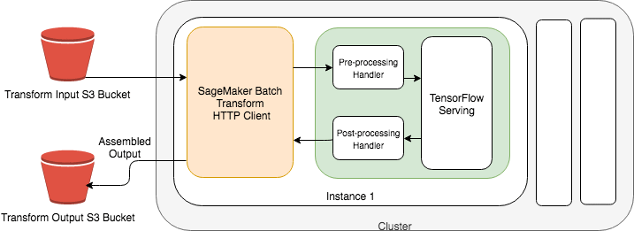
Figure 6-21. Pre-Processing Request Handler and Post-Processing Response Handler
We start with the input_handler function. Note that the code looks very similar to the code we used in the feature engineering chapter. The input_handler function converts batches of raw text into BERT tokens using the Transformer library.
import json
import tensorflow as tf
from transformers import DistilBertTokenizer
review_body_column_idx_tsv = 13
classes=[1, 2, 3, 4, 5]
max_seq_length=128
tokenizer = DistilBertTokenizer.from_pretrained('distilbert-base-uncased')
def input_handler(data, context):
  transformed_instances = []
  for instance in data:
    data_str = instance.decode('utf-8')
    data_str_split = data_str.split('	')
    print(len(data_str_split))
    if (len(data_str_split) >= review_body_column_idx_tsv):
      print(data_str_split[review_body_column_idx_tsv])
    text_input = data_str_split[review_body_column_idx_tsv]
    tokens = tokenizer.tokenize(text_input)
    encode_plus_tokens = tokenizer.encode_plus(text_input,
                          pad_to_max_length=True,
                          max_length=max_seq_length)
    # Convert the text-based tokens to ids from the pre-trained BERT vocabulary
    input_ids = encode_plus_tokens['input_ids']
    # Specifies which tokens BERT should pay attention to (0 or 1)
    input_mask = encode_plus_tokens['attention_mask']
    # Segment Ids are always 0 for single-sequence tasks (or 1 if two-sequence tasks)
    segment_ids = [0] * max_seq_length

    transformed_instance = {
                 "input_ids": input_ids,
                 "input_mask": input_mask,
                 "segment_ids": segment_ids
                }

    transformed_instances.append(transformed_instance)
  transformed_data = {"instances": transformed_instances}  return json.dumps(transformed_data)
SageMaker then passes this batched output from the input_handler into our model which produces batches of predictions. The predictions are passed through the output_handler function which converts the prediction into a json response. SageMaker then joins each prediction within a batch to its specific line of input. This produces a single, coherent line of output for each row that was passed in.
def output_handler(response, context):
  response_json = response.json()
  log_probabilities = response_json["predictions"]
  predicted_classes = []
  for log_probability in log_probabilities:
    softmax = tf.nn.softmax(log_probability)
    predicted_class_idx = tf.argmax(softmax, axis=-1, output_type=tf.int32)
    predicted_class = classes[predicted_class_idx]
    predicted_classes.append(predicted_class)
  predicted_classes_json = json.dumps(predicted_classes)
  response_content_type = context.accept_header  return predicted_classes_json, response_content_type
Run the Batch Transformation Job
Next we will specify the input data and start the actual batch transformation job. Note that our input data is compressed using Gzip as Batch Transformation Jobs support many types of compression.
batch_predictor.transform(data=input_csv_s3_uri,
             split_type=split_type,
             compression_type=compression_type,
             content_type=content_type,
				  join_source='Input',
             experiment_config=None,
             wait=False)
We specify join_source='Input' to force SageMaker to join our prediction with the original input before writing to S3. And while not shown here, SageMaker lets you specify the exact input features to pass into this batch transformation process using InputFilter and the exact data to write to S3 using OutputFilter. This helps to reduce overhead, reduce cost, and improve batch prediction performance.
If you are using join_source='Input' and InputFilter together, SageMaker will join the original inputs - including the filtered-out inputs - with the predictions to keep all of the data together. You can also filter the outputs to reduce the size of the prediction files written to S3. The whole flow is shown in Figure 6-22.

Figure 6-22. : Filtering and Joining Inputs to Reduce Overhead and Improve Performance
Review the Batch Predictions
Once the Batch Transform Job completes, we can review the generated comma-separated .out files that contain our review_body inputs and star_rating predictions as shown here:
amazon_reviews_us_Digital_Software_v1_00.tsv.gz.outamazon_reviews_us_Digital_Video_Games_v1_00.tsv.gz.out
Here are a few sample predictions:
'This is the best movie I have ever seen', 5,'Star Wars''This is an ok, decently-funny movie.', 3,'Spaceballs''This is the worst movie I have ever seen', 1,'Star Trek'
At this point, we have performed a large number of predictions and generated comma-separated output files. With a little bit of application code (SQL, Python, Java, etc), we can use these predictions to power natural-language-based applications to improve the customer service experience, for example.
Lambda Functions and API Gateway
You can also deploy your models as serverless APIs with AWS Lambda. When a prediction request arrives, the Lambda function loads the model from S3 and executes the inference function code. You can use the “provisioned concurrency” feature of Lambda to pre-load the model into the function and greatly improve prediction latency. Amazon API Gateway provides additional support for application authentication, authorization, caching, rate-limiting, and web application firewall (WAF) rules. Figure 6-23 shows how you implement serverless inference with AWS Lambda and API Gateway

Figure 6-23. Serverless inference with AWS Lambda and API Gateway
Note
At the time of this writing, AWS Lambda functions had some limitations including no GPU support and limited model size. If your model is not affected by those restrictions, AWS Lambda is a viable model deployment option.
Reduce Costs and Increase Performance
In this section, we describe multiple ways to reduce cost and increase performance by packing multiple models into a single SageMaker deployment container, utilizing GPU-based Elastic Inference Adapters, optimizing your trained model for specific hardware, and utilizing inference-optimized hardware such as the Amazon Inferentia chip.
Deploy Multiple Models in One Container
If you have a large number of similar models that you can serve through a shared serving container - and don’t need to access all the models at the same time - you can use SageMaker’s multi-model jendpoint (MME) capability. When there is a long tail of ML models that are infrequently accessed, using one multi-model endpoint can efficiently serve inference traffic and enable significant cost savings.
Multi-model endpoints can automatically load and unload models based on traffic and resource utilization. For example, if traffic to model1 goes to zero and model2 traffic spikes, SageMaker will dynamically unload model1 and load another instance of model2.
While MME lets you deploy multiple models to a single endpoint and serve them using a single container, you can invoke a specific model by specifying the target model name as a parameter in your prediction request as shown in Figure 6-24.
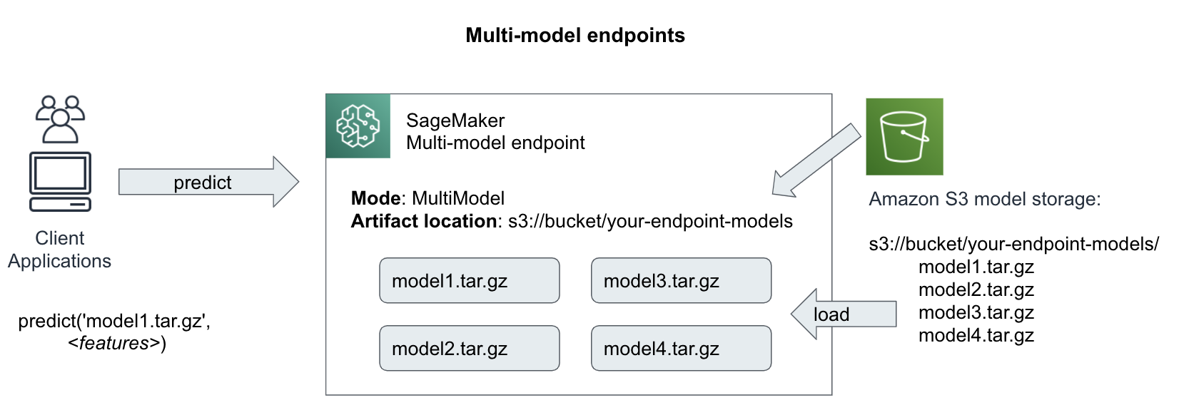
Figure 6-24. Invoke a specific model with multi-model endpoints
Here is the code to deploy two(2) TensorFlow models behind a single endpoint. The most human-grokkable use case here is when a practitioner has trained multiple for slightly differently audiences (ie. Audi lovers model1, Porsche lovers model2), but wants to deploy them to the same endpoint for convenience and cost purposes.
For TensorFlow, we need to package the models as follows:
└── multi
  ├── model1
  │  └── <version number>
  │    ├── saved_model.pb
  │    └── variables
  │      └── ...
  └── model2
    └── <version number>
      ├── saved_model.pb
      └── variables
        └── ...
from sagemaker.tensorflow.serving import Model, Predictor
# For multi-model endpoints, you should set the default
#  model name in this environment variable.
# If it isn't set, the endpoint will work, but the model
#  it will select as default is unpredictable.
env = {
 'SAGEMAKER_TFS_DEFAULT_MODEL_NAME': 'model1' # <== This must match the directory
}
model_data = '{}/multi.tar.gz'.format(multi_model_s3_uri)
model = Model(model_data=model_data,
       role=role,
       framework_version='2.1.0',        env=env)
Attach a GPU-based Elastic Inference Accelerator
Elastic Inference Accelerator (EIA) is a low-cost, dynamically-attached, GPU-powered add-on for SageMaker instances. While standalone GPU instances are a good fit for model training on large datasets, they are typically oversized for smaller-batch inference requests which consume small amounts of GPU resources.
While AWS offers a wide range of instance types with different GPU, CPU, network bandwidth, and memory combinations, your model may use a custom combination. With EIA’s, you can start by choosing a base CPU instance and add GPUs until you find the right balance for your model inference needs. Otherwise, you may be forced to optimize one set of resources like CPU and RAM, but underutilize other resources like GPU and network bandwidth.
Here is the code to deploy our same model but with an Elastic Inference Accelerator (EIA).
import time
timestamp = '{}'.format(int(time.time()))
endpoint_config_name = '{}-{}'.format(training_job_name, timestamp)
variantA = production_variant(model_name='ModelA',                              instance_type="ml.m5.large",
                              initial_instance_count=1,
                              variant_name='VariantA',
                              initial_weight=50,
   accelerator_type='ml.eia2.medium')
variantB = production_variant(model_name='ModelB',
                              instance_type="ml.m5.large",
                              initial_instance_count=1,
                              variant_name='VariantB',
                              initial_weight=50)
endpoint_config = sm.create_endpoint_config(
  EndpointConfigName=endpoint_config_name,
  ProductionVariants=[variantA, variantB]
)
endpoint_name = '{}-{}'.format(training_job_name, timestamp)
endpoint_response = sm.create_endpoint(
  EndpointName=endpoint_name,
  EndpointConfigName=endpoint_config_name)
Optimize a Trained Model with SageMaker Neo and TensorFlow Lite
SageMaker Neo takes a trained model and performs a series of hardware-specific optimizations such as 16-bit quantization, graph pruning, layer fusing, and constant folding for instant 2x model-prediction speedups with minimal accuracy loss. Neo works across popular AI and machine learning frameworks including TensorFlow, PyTorch, MXNet, and XGBoost.
Neo parses the model, optimizes the graph, quantizes tensors, and generates hardware-specific code for a variety of target environments including Intel x86 CPUs, Nvidia GPUs, and Amazon Inferentia as shown in Figures 9-25.

Figure 6-25. Parsing Models, Optimizing Graphs and Tensors, and Generating Hardware-Specific Code
SageMaker Neo supports TensorFlow Lite (TF Lite), a highly-optimized TensorFlow code generator. Neo uses the TF Lite converter to perform hardware-specific optimizations for the The TensorFlow Lite interpreter as shown in Figure 6-26.
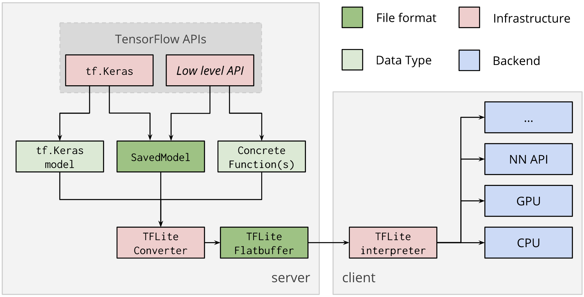
Figure 6-26. TF Lite interpreter (Source: https://www.tensorflow.org/lite/convert)
Here is the TF Lite code that performs 16-bit quantization on a TensorFlow model.
import tensorflow as tfconverter = tf.lite.TocoConverter.from_saved_model('./tensorflow/')converter.post_training_quantize = Truetflite_model = converter.convert()tflite_model_path = './tflite/tflite_optimized_model.tflite'model_size = open(tflite_model_path, "wb").write(tflite_model)
Here’s the prediction code that leads to an order-of-magnitude speed up in prediction time due to the quantization:
import numpy as npimport tensorflow as tf# Load TFLite model and allocate tensors.interpreter = tf.lite.Interpreter(model_path=tflite_model_path)interpreter.allocate_tensors()# Get input and output tensors.input_details = interpreter.get_input_details()output_details = interpreter.get_output_details()# Test model on random input data.input_shape = input_details[0]['shape']input_data = np.array(np.random.random_sample(input_shape),dtype=np.float32)interpreter.set_tensor(input_details[0]['index'], input_data)interpreter.invoke()output_data = interpreter.get_tensor(output_details[0]['index'])print('Prediction: %s' % output_data)
Use Inference-Optimized Hardware
AWS Inferentia is an inference-optimized chip designed to accelerate 16-bit and 8-bit floating point operations generated by SageMaker Neo’s Inferentia-specific optimizer called Neuron as shown in Figure 6-27.
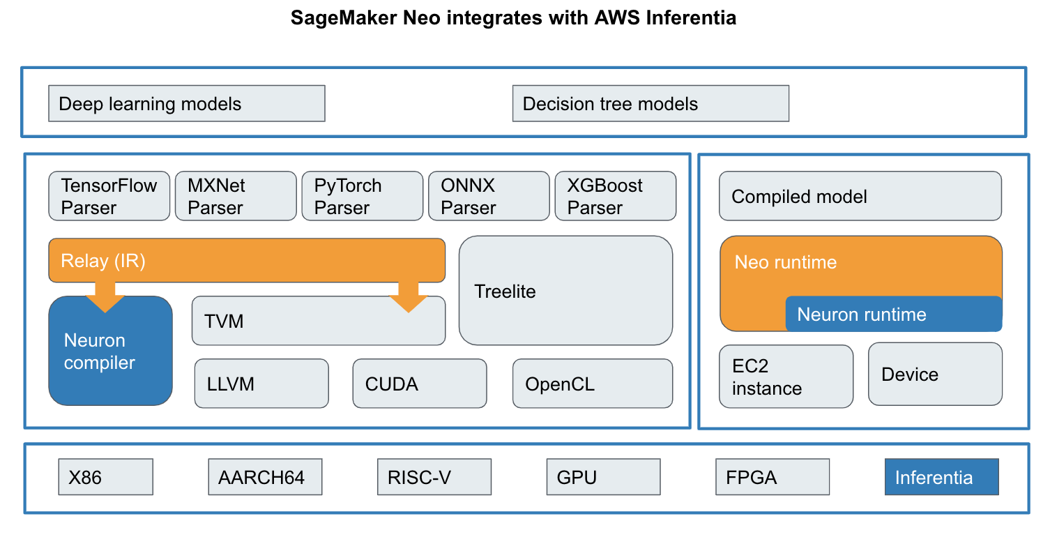
Figure 6-27. SageMaker Neo’s Neuron Optimizer for AWS Inferentia Chip
Summary
In this chapter, we moved our models out of the research lab and into the end-user application domain. We can now measure, and improve, and deploy our models using real-world, production-ready fundamentals such as canary rollouts, blue/green deployments, A/B tests, drift detection, and lineage tracking. In addition, we performed batch transformations to improve throughput for offline model predictions. We closed out with tips on how to reduce cost and improve performance using SageMaker Neo, TensorFlow Lite, SageMaker Multi-Model Endpoints and inference-optimized hardware such as Elastic Inference Accelerator (EIA) and Amazon Inferentia.