Trace and Audit Model Lineage

Humans are naturally curious. When presented with an object, people will likely want to know how that object was created. Now consider an object as powerful and mysterious as a predictive model learned by a machine. We naturally want to know how this model was created. Which dataset was used? Which hyper-parameters were chosen? Which other hyper-parameters were explored? How does this version of the model compare to the previous version? All of these questions can be answered by SageMaker Experiments.

The SageMaker Experiments feature brings traceability, lineage tracking, and auditability to your AI and machine learning workflows. Users can quickly traceback the entire model lineage using the Experiments API. In addition, all SageMaker and S3 API calls are logged as private CloudTrail and CloudWatch logs for fine-grained and secure auditing.

Reproduce a Model

Reproducibility is critical to understanding how a model was trained including the data sets, algorithm, and hyper-parameters involved. Along with traceability and auditability, SageMaker Experiments provide full model reproducibility by allowing practitioners to restore everything including the train/validation/test datasets, algorithm, hyper-parameters, and trained model.

However, remember that AI and machine learning models are stochastic vs. deterministic and therefore difficult to reproduce model results exactly. Still, reproducibility is critical to understanding how a model was trained including the data sets, algorithm, and hyper-parameters involved.

Manage Artifacts and Dependencies

We can use the log_artifact() Experiment API to save, version, and restore all model artifacts in either S3 or Git. Users should enable S3 versioning and object locking to maintain artifacts for reproducibility and auditability.

Dependencies such as Python libraries and Docker images should always be retrieved from private, internal artifact repositories such as AWS CodeCommit and Elastic Container Registry (ECR) to reduce security risks and increase performance. Any dependency pulled from the Internet may slow down the training job and potentially introduce security risks. If a dependency is not available due to a temporary outage or throttling event with external dependency providers like PyPi, Maven, GitHub, or DockerHub, your training cluster will fail.

Track Our Model Lifecycle with the Experiments API

The SageMaker Experiments API is made up of a few key abstractions as follows:

Experiment

A collection of related Trials. Add Trials to an Experiment that you wish to compare together.

Trial

A description of a multi-step machine learning workflow. Each step in the workflow is described by a Trial Component.

Trial Component

A description of a single step in a machine learning workflow. For example data cleaning, feature extraction, model training, model evaluation, etc.

Tracker

A logger of information about a single TrialComponent.

You can use SageMaker Experiments from any Jupyter notebook or Python script by using the SageMaker Experiments Python SDK and adding a few lines of code to setup and track the experiment.

Let’s say we want to improve upon our model from the training run in the previous chapter. We will call this Model A and place it into Trial A within Experiment A as shown in Figure 5-2. Next, we create two(2) additional trials, Trials B and C, which use different sets of hyper-parameters to train two(2) separate models, Models B and C, respectively.

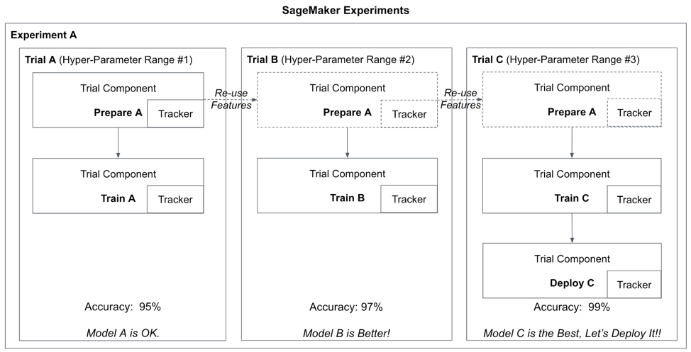
Figure 5-2. : Compare training runs with different hyper-parameters using SageMaker Experiments

Using the SageMaker Experiments API, we create a complete record of every step and hyper-parameter used to re-create Models A, B, and C. Later, we will extend this lineage to include model deployment.

At any given point in time, we should be able to trace a model back to its origins including the exact dataset used to train the model. This traceability is essential for auditing, explaining, and improving your models.

Set Up the Experiment

Let’s modify our training script to use the SageMaker Experiment API to track the lineage of our BERT-based review classifier model that we built in the previous chapter. Let’s first create our Experiment.

import time
from smexperiments.experiment import Experiment
timestamp = '{}'.format(int(time.time()))
experiment = Experiment.create(
                experiment_name='Amazon-Customer-Reviews-BERT-Experiment-{}'.format(timestamp),
                description='Amazon Customer Reviews BERT Experiment', 
                sagemaker_boto_client=sm)
experiment_name = experiment.experiment_name
print('Experiment name: {}'.format(experiment_name))

Next, we add a Trial to the experiment and Tracker the feature engineering configuration including the S3 locations of the raw_input and train/validation/test datasets - as well as the BERT max_seq_length used during tokenization.

import time
from smexperiments.trial import Trial
timestamp = '{}'.format(int(time.time()))
trial = Trial.create(trial_name='trial-{}'.format(timestamp),
                     experiment_name=experiment_name,
                     sagemaker_boto_client=sm)
trial_name = trial.trial_name
print('Trial name: {}'.format(trial_name))
from smexperiments.tracker import Tracker
tracker_prepare = Tracker.create(display_name='prepare', 
                                 sagemaker_boto_client=sm)
prepare_trial_component_name = tracker_prepare.trial_component.trial_component_name
print('Prepare trial component name {}'.format(prepare_trial_component_name))
trial.add_trial_component(tracker_prepare.trial_component)
tracker_prepare.log_input(name='raw_data_s3_uri', 
                          media_type='s3/uri', 
                          value=s3_raw_input_data)
tracker_prepare.log_parameters({
    'max_seq_length': max_seq_length,
    'train_split_percentage': train_split_percentage,
    'validation_split_percentage': validation_split_percentage,
    'test_split_percentage': test_split_percentage,
})
tracker_prepare.log_output(name='train_data_s3_uri', 
                           media_type='s3/uri', 
                           value=processed_train_data_s3_uri)
tracker_prepare.log_output(name='validation_data_s3_uri', 
                           media_type='s3/uri', 
                           value=processed_validation_data_s3_uri)
tracker_prepare.log_output(name='test_data_s3_uri', 
                           media_type='s3/uri', 
                           value=processed_test_data_s3_uri)
tracker_prepare.trial_component.save()

Next, let’s configure the experiment_config parameter that we will pass to the TensorFlow.fit() function when we train our model. This experiment_confi is used by SageMaker to update the new TrialComponen and Tracker created during training called train.

experiment_config = {
    'ExperimentName': experiment_name,
    'TrialName': trial.trial_name,
    'TrialComponentDisplayName': 'train'
}

Here is the modified call to the TensorFlow.fit() function to track the train trial:

estimator.fit(inputs={'train': s3_input_train_data, 
                     		'validation': s3_input_validation_data,
                      	'test': s3_input_test_data
     		        },              
              	   experiment_config=experiment_config,                   
              	   wait=False)

Here is how we compare the experiment trials:

from sagemaker.analytics import ExperimentAnalytics
lineage_table = ExperimentAnalytics(
    sagemaker_session=sess,
    experiment_name=experiment_name,
    metric_names=['validation:accuracy'],
    sort_by="CreationTime",
    sort_order="Ascending",
)
lineage_df = lineage_table.dataframe()
lineage_df

Below are the values logged by our prepare tracker as well as the train tracker created by SageMaker during training.

TrialComponentName	DisplayName	max_seq_length	learning_rate	...
TrialComponent-2020-06-13-062410-pxuy	prepare	128.0	NaN	...
tensorflow-training-2020-06-13-06-24-12-989	train	128.0	0.00001	...

Set Up the Hyper-Parameter Ranges

First, let’s create an optimize tracker and associate it with our experiment.

from smexperiments.tracker import Tracker
tracker_optimize = Tracker.create(display_name='optimize-1', 
                                  sagemaker_boto_client=sm)
optimize_trial_component_name = 
tracker_optimize.trial_component.trial_component_name
trial.add_trial_component(tracker_optimize.trial_component)

To keep this example simple and avoid a combinatorial explosion of trial runs, we will freeze most hyper-parameters and explore only a limited set for this particular optimization run. In a perfect world with unlimited resources and budget, we would explore every combination of hyper-parameters. For now, we will freeze the following:

epochs=1
epsilon=0.00000001
train_batch_size=128
validation_batch_size=128
test_batch_size=128
train_steps_per_epoch=50
validation_steps=50
test_steps=50
use_xla=True
use_amp=True
freeze_bert_layer=True

Next, let’s set up the hyper-parameter ranges that we wish to explore. We are choosing these hyper-parameters based on intuition, domain knowledge, and algorithm documentation. You may also find research papers useful - or other prior work from others in the community. At this point in the life cycle of machine learning and predictive analytics, you can almost-always find relevant information on the problem you are trying to solve.

If you still can’t find a suitable starting point, you should explore ranges logarithmically (vs. linearly) to help gain a sense of the scale of the hyper-parameter. There is no point in exploring the set [1, 2, 3, 4] if your best hyper-parameter is orders of magnitude away in the 1,000’s, for example.

SageMaker Autopilot is another way to determine a baseline set of hyper-parameters for your algorithm and dataset. Autopilot’s hyper-parameter selection process has been refined on many thousands of hours of training jobs across a wide range of data sets, algorithms, and use cases within Amazon.

SageMaker hyper-parameter tuning supports three types of parameter ranges:

Categorical(list)

Hyper-Parameters that have a discrete list of possible values.

ContinuousParameter(min, max): Hyper-Parameters that have a continuous range of possible values.

IntegerParameter (min, max)

Hyper-Parameters that have an integer range of possible values.

Here we are specifying defining learning_rate as a ContinuousParameter:
from sagemaker.tuner import IntegerParameter
from sagemaker.tuner import ContinuousParameter
from sagemaker.tuner import CategoricalParameter
from sagemaker.tuner import HyperparameterTuner
                                                
hyperparameter_ranges = {
    'learning_rate': ContinuousParameter(0.00001, 0.00005, scaling_type='Linear'),
}

You can also specify the scaling type for each type of hyper-parameter ranges. The scaling type can be set to Linear, Logarithmic, ReverseLogarithmic, or Auto to allow SageMaker to decide.

Finally, we need to define the objective metric that the hyper-parameter tuning job is trying to optimize - in our case, validation accuracy. Remember that we need to provide the regular expression (regex) to extract the metric from the SageMaker container logs. We chose to also collect the training loss, training accuracy, and validation loss for informational purposes.

objective_metric_name = 'validation:accuracy'
metrics_definitions = [
     {'Name': 'train:loss', 'Regex': 'loss: ([0-9\.]+)'},
     {'Name': 'train:accuracy', 'Regex': 'accuracy: ([0-9\.]+)'},
     {'Name': 'validation:loss', 'Regex': 'val_loss: ([0-9\.]+)'},
     {'Name': 'validation:accuracy', 'Regex': 'val_accuracy: ([0-9\.]+)'}]

Run the Hyper-Parameter Tuning Job

We start by creating our TensorFlow estimator similar to the previous chapter. Note that we are not specifying the learning_rate hyper-parameter in this case. We will pass this as a hyper-parameter range to the HyperparameterTuner in a moment.

from sagemaker.tensorflow import TensorFlow
estimator = TensorFlow(entry_point='tf_bert_reviews.py',
                       source_dir='src',
                       role=role,
                       train_instance_count=train_instance_count,
                       train_instance_type=train_instance_type,
                       py_version='py3',
                       framework_version='2.1.0',
                       hyperparameters={'epochs': epochs,
                                        'epsilon': epsilon,
                                        'train_batch_size': train_batch_size,
                                        'validation_batch_size': validation_batch_size,
                                        'test_batch_size': test_batch_size,                                             
                                        'train_steps_per_epoch': train_steps_per_epoch,
                                        'validation_steps': validation_steps,
                                        'test_steps': test_steps,
                                        'use_xla': use_xla,
                                        'use_amp': use_amp,
                                        'max_seq_length': max_seq_length,
                                        'freeze_bert_layer': freeze_bert_layer,
                       metric_definitions=metrics_definitions,
                      )

Next, we can create our Hyper-Parameter Tuning Job by passing the TensorFlow estimator, hyper-parameter range, objective metric, tuning strategy, number of jobs to run in parallel/total, as well as an early stopping strategy. SageMaker will use the given optimization strategy (ie. “Bayesian” or “Random Search”) to explore the values within the given ranges.

objective_metric_name = 'validation:accuracy'
tuner = HyperparameterTuner(
    estimator=estimator,
    objective_type='Maximize',
    objective_metric_name=objective_metric_name,
    hyperparameter_ranges=hyperparameter_ranges,
    metric_definitions=metrics_definitions,
    max_jobs=100,
    max_parallel_jobs=10,
    strategy='Bayesian',
    early_stopping_type='Auto'
)

In this example, we are using the Bayesian optimization strategy and with 10 jobs in parallel and 100 total. By only doing 10 at a time, we give the Bayesian strategy a chance to learn from previous runs. In other words, if we did all 100 in parallel, the Bayesian strategy could not use prior information to choose better values within the ranges provided.

By setting early_stopping_type to 'Auto', SageMaker will stop the tuning job if the tuning job is not going to improve upon the objective metric.  This helps save time and reduce the overall cost of your tuning job.
Let’s start the tuning job by calling tuner.fit() and pointing to our training data input channels:  
tuner.fit(inputs={'train': s3_input_train_data, 
                  'validation': s3_input_validation_data,
                  'test': s3_input_test_data
          }, 
          include_cls_metadata=False)

Using our experiment tracker, let’s update the experiment lineage to include the best hyper-parameters and objective metrics found by our hyper-parameter tuning job.

tracker_optimize.log_parameters({ 
'learning_rate': best_learning_rate
})
tracker_optimize.log_metrics({ 
'validation:accuracy': best_validation_accuracy
})
tracker_optimize.trial_component.save()

Analyze the Tuning Job Results

Once the hyper-parameter tuning job has finished, we can analyze the results directly in our notebook or through SageMaker Studio.

from sagemaker.analytics import ExperimentAnalytics
lineage_table = ExperimentAnalytics(
    sagemaker_session=sess,
    experiment_name=experiment_name,
    metric_names=['validation:accuracy'],
    sort_by="CreationTime",
    sort_order="Ascending",
)
lineage_df = lineage_table.dataframe()
lineage_df

The output should look similar to this:

TrialComponentName	DisplayName	max_seq_length	learning_rate	validation_accuracy	...
TrialComponent-2020-06-13-062410-pxuy	prepare	128.0	NaN	NaN	...
tensorflow-training-2020-06-13-06-24-12-989	train	128.0	0.00001	0.7420	...
TrialComponent-2020-06-12-193933-bowu	optimize-1	128.0	0.000017	0.7824	...

In this case, the learning_rate value of 0.000017 gives the highest validation accuracy of 0.7824.

We can also view details of the best candidate directly in the SageMaker UI as shown in Figure 5-4.

Figure 5-4. Details of the best candidate.

The CloudWatch system and algorithms metrics for one of the tuning jobs is shown in Figure 5-5.

Figure 5-5. CloudWatch System and Algorithm Performance Metrics for a Tuning Job

We can also view the complete list of all parallel tuning jobs as shown in Figure 5-6. Note that some completed successfully and some were stopped early to save time and reduce cost.

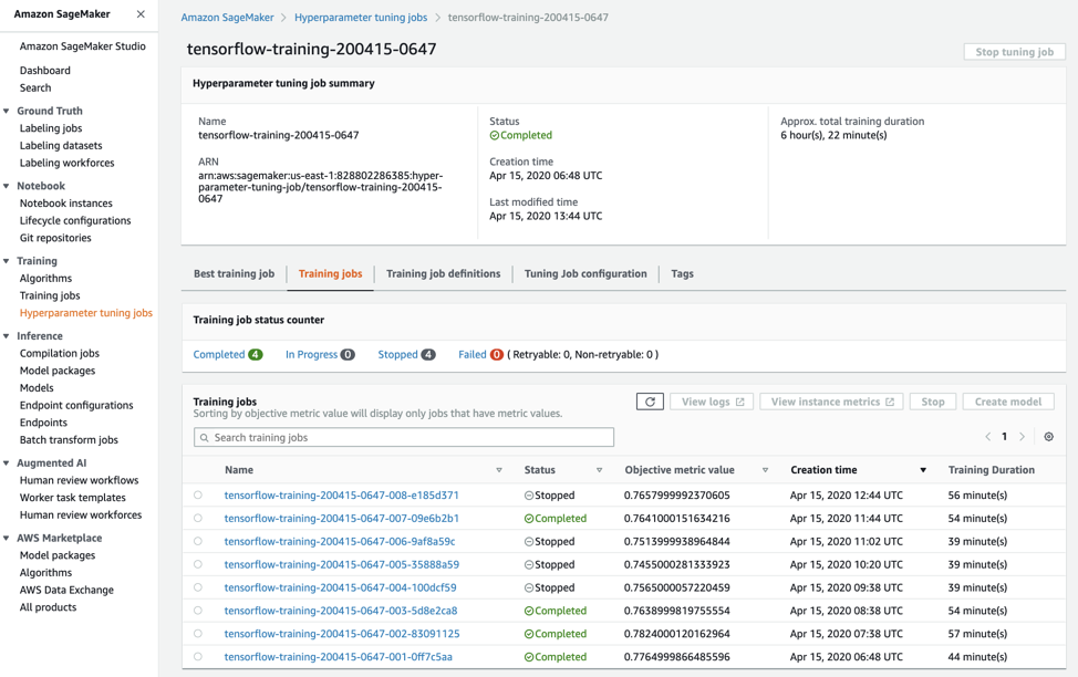
Figure 5-6. List of Tuning Jobs.

In this example, we have optimized the hyper-parameters of our TensorFlow BERT classifier layer. SageMaker hyper-parameter tuning also supports automatic hyper-parameter tuning across multiple algorithms by adding a list of algorithms to the tuning job definition. You can specify different hyper-parameters and ranges for each algorithm. SageMaker Autopilot automatically uses multi-algorithm tuning to find the best model across many different algorithms based on your dataset and objective function.

Run Hyper-Parameter Tuning Job using Warm Start

We need to configure the tuning job with the WarmStartConfig using one or more of the previous hyper-parameter tuning jobs as parents. The parent HPT jobs must have finished either with one of the following success or failure states: Completed, Stopped, or Failed. Recursive parent-child relationships are not supported. We also need to specify the WarmStartType. In our example, we will use the IDENTICAL_DATA_AND_ALGORITHM as we plan to only modify the hyper-parameter ranges and not use an updated dataset or algorithm version.

Let’s start with the setup of the WarmStartConfig:

from sagemaker.tuner import WarmStartConfig
from sagemaker.tuner import WarmStartTypes
warm_start_config = 
WarmStartConfig(warm_start_type=WarmStartTypes.IDENTICAL_DATA_AND_ALGORITHM, 
 parents={tuning_job_name})

Let’s define the static hyper-parameters that we are not planning to explore.

epochs=1
epsilon=0.00000001
train_batch_size=128
validation_batch_size=128
test_batch_size=128
train_steps_per_epoch=50
validation_steps=50
test_steps=50
use_xla=True
use_amp=True
freeze_bert_layer=True
from sagemaker.tensorflow import TensorFlow
estimator = TensorFlow(entry_point='tf_bert_reviews.py',
                       source_dir='src',
                       role=role,
                       train_instance_count=train_instance_count, 
                       train_instance_type=train_instance_type,
                       train_volume_size=train_volume_size,
                       py_version='py3',
                       framework_version='2.1.0',
                       hyperparameters={'epochs': epochs,
                                        'epsilon': epsilon,
                                        'train_batch_size': train_batch_size,
                                        'validation_batch_size': validation_batch_size,
                                        'test_batch_size': test_batch_size,                                             
                                        'train_steps_per_epoch': train_steps_per_epoch,
                                        'validation_steps': validation_steps,
                                        'test_steps': test_steps,
                                        'use_xla': use_xla,
                                        'use_amp': use_amp,
                                        'max_seq_length': max_seq_length,
                                        'freeze_bert_layer': freeze_bert_layer	 

}

                       metric_definitions=metrics_definitions,
                      )

While we can choose to explore more hyper-parameters in this warm start tuning job, we will simply modify the range of our learning_rate to narrow in on the best value found in the parent tuning job.

from sagemaker.tuner import IntegerParameter
from sagemaker.tuner import ContinuousParameter
from sagemaker.tuner import CategoricalParameter
                                                
hyperparameter_ranges = {
    'learning_rate': ContinuousParameter(0.00015, 0.00020,
						  	   scaling_type='Linear')}

Now let’s define the objective metric, create the HyperparameterTuner with the warm_start_config from above, and start the tuning job.

objective_metric_name = 'validation:accuracy'
tuner = HyperparameterTuner(
    estimator=estimator,
    objective_type='Maximize',
    objective_metric_name=objective_metric_name,
    hyperparameter_ranges=hyperparameter_ranges,
    metric_definitions=metrics_definitions,
    max_jobs=2,
    max_parallel_jobs=1,
    strategy='Bayesian',
    early_stopping_type='Auto',
    warm_start_config=warm_start_config
)
tuner.fit({'train': s3_input_train_data, 
           'validation': s3_input_validation_data,
           'test': s3_input_test_data}, 
          include_cls_metadata=False)

Figure 5-8 shows the results of the warm start hyper parameter tuning job in the SageMaker UI. We see that 7 out of 8 tuning jobs stopped early because they could not beat the accuracy of the parent’s best candidate.

Figure 5-8. Result of the Warm Start Hyper-Parameter Tuning Job in the SageMaker UI.

And the tuning job that completed successfully did not beat the accuracy of the parent’s best candidate, either. Therefore, the hyper-parameter found from the parent tuning is still the best candidate as shown in Figure 5-9.

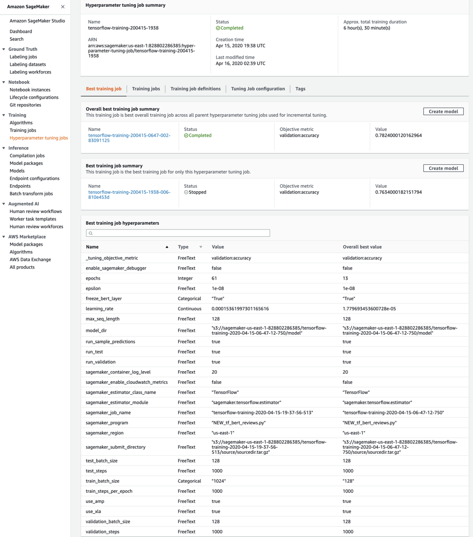
Figure 5-9. The Warm Start Tuning Job Does Not Beat the Accuracy of the Parent Tuning Job

Increase Cluster Instance Count

SageMaker, following cloud-native principles, is inherently distributed and scalable in nature. In the previous chapter, we were using a single instance by specifying train_instance_count=1. Simply by increasing the train_instance_count > 1, we will enable SageMaker distributed training as shown below.

train_instance_count=3
train_instance_type='ml.p3dn.24xlarge'
from sagemaker.tensorflow import TensorFlow
estimator = TensorFlow(entry_point='tf_bert_reviews.py', 
                     	source_dir='src', 
train_instance_count=train_instance_count,                        
train_instance_type=train_instance_type,
...
                     	py_version='py3',
                     	framework_version='2.1.0')

SageMaker automatically passes the relevant cluster-environment information to TensorFlow to enable distributed TensorFlow. Our TensorFlow code does not change at all. SageMaker passes the same cluster-environment information to other distributed machine learning frameworks such as PyTorch and MXNet.

Choose an Appropriate Cluster Communication Strategy

The instances communicate and share their learnings throughout the training process. This communication benefits from a high-bandwidth connection between the cluster instances. And the instances should be physically close to each other in the cloud data center. Fortunately, SageMaker handles all of the heavy lifting for you so you can stay focused on the business problem you’re trying to solve.

“Parameter server” is a primitive distributed training strategy supported by most distributed machine learning frameworks. Reminder that parameters are what the algorithm is learning. Hyper-parameters control how the algorithm learns these parameters. When performing distributed training across many cluster instances, we need a central place to store the parameters learned by all the nodes in the cluster as shown in Figure 5-10.

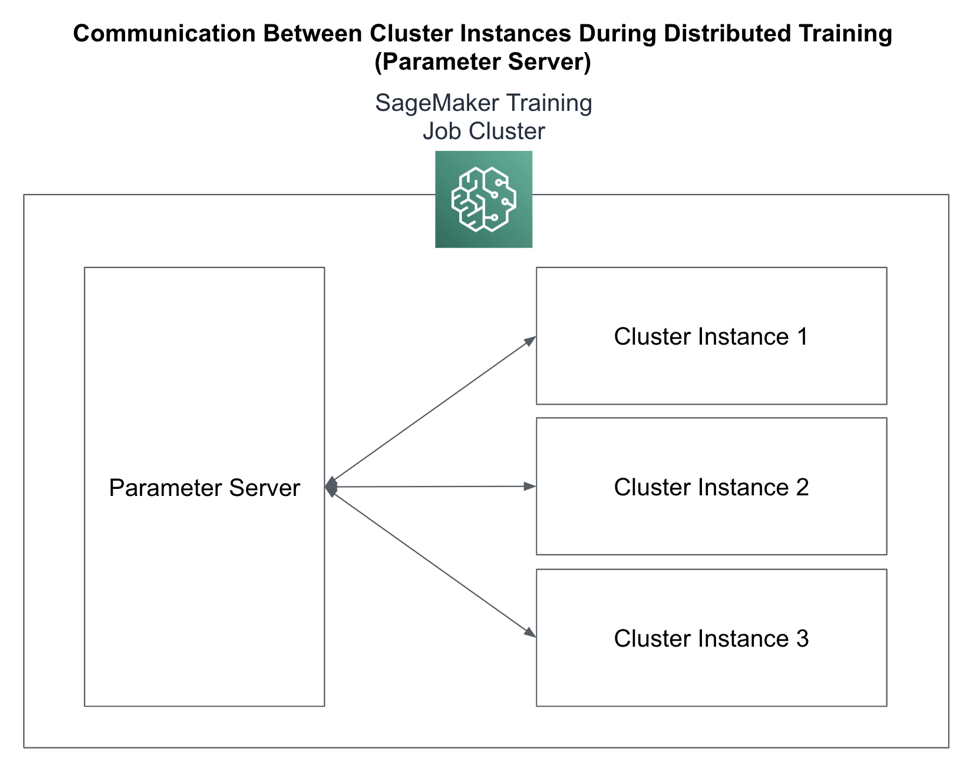
Figure 5-10. : Parameter Server Cluster Communication Strategy

Because they perform relatively lightweight computations, parameter server clusters are typically CPU-based instances while the worker cluster uses GPUs to perform the heavyweight, algorithm-specific computations and numerical optimizations. It’s also important to note that parameter server clusters are stateful while worker clusters are stateless. This is an important distinction when evaluating failover-recovery situations and spot-instance configurations.

Another common distributed communication strategy rooted in parallel computing and message-passing interfaces (MPI) is “all reduce.” All reduce uses a ring-like communication pattern as shown in Figure 5-11 which helps to reduce the single-point-of-failure of the parameter server and increase overall training efficiency.

Figure 5-11. : AllReduce Cluster Communication Strategy

Continuing with our TensorFlow example, we will leverage the MultiWorkerMirroredStrategy which uses the all reduce distributed communication strategy across many instances in our cluster.

distributed_strategy = 
tf.distribute.MultiWorkerMirroredStrategy()
with distributed_strategy.scope():
	loss = 
tf.keras.losses.SparseCategoricalCrossentropy(from_logits=True)
     metric = 
tf.keras.metrics.SparseCategoricalAccuracy('accuracy')
     model.compile(optimizer=optimizer, 
  loss=loss, 
  metrics=[metric])
		...

Cache S3 Data using FSx for Lustre

Amazon FSx for Lustre is a high-performance, POSIX-compatible file system that natively integrates with S3. FSx for Lustre is based on the open source Lustre file system designed for highly scalable, highly distributed, and highly parallel training jobs with petabytes of data, terabytes per second of aggregate I/O throughput, and consistent low-latency.

There is also FSx for Windows which provides a Windows-compatible file system that natively integrates with S3, as well. However, we have chosen to focus on FSx for Lustre as our examples are Linux-based. Both file systems are optimized for machine learning, analytics, and high performance computing workloads using S3. And both file systems offer similar features.

FSx for Lustre is a fully-managed service that simplifies the complexity of setting up and managing the Lustre File System. Mounting an S3 bucket as a file system in minutes, FSx for Lustre lets you access data from any number of instances concurrently. FSx for Lustre caches S3 objects to improve performance of iterative machine learning workloads that pass over the dataset many times to fit a high-accuracy model. Figure 8-12 shows how SageMaker uses FSx for Lustre to provide fast, shared access to your S3 data and accelerate your training and tuning jobs. Your SageMaker training cluster instances access a file in FSx for Lustre using /mnt/data/file1.txt. FSx for Lustre translates this request and issues a GetObject request to S3. The file is cached and returned to the cluster instance. If the file has not changed, subsequent requests will return from FSx for Lustre’s cache. Since training data does not typically change during a training job run, we see huge performance gains as we iterate through our dataset over many training epochs.

Figure 5-12. SageMaker Uses FSx for Lustre to Increase Training and Tuning Job Performance

Once you have set up the FSx for Lustre file system, you can pass the location of the FSx for Lustre file system into the training job as follows:

estimator = TensorFlow(entry_point='tf_bert_reviews.py', 
                       source_dir='src', 
                       train_instance_count=train_instance_count,
                       train_instance_type=train_instance_type,
                       subnets=['subnet-1', 'subnet-2']
                       security_group_ids=['sg-1'])
fsx_data = FileSystemInput(file_system_id='fs-1',
                           file_system_type='FSxLustre',
                           directory_path='/mnt/data,
                           file_system_access_mode='ro')
estimator.fit(inputs=fsx_data)

Share Data using Elastic File System

While many SageMaker optimizations exist for reading training data from S3, there are also optimizations for reading data from Amazon’s Elastic File System (EFS), an implementation of the standard Network File System (NFS) optimized for AWS’s cloud-native and elastic environment. EFS provides centralized, shared access to your training data sets across thousands of instances in a distributed training cluster as shown in Figure 5-13.

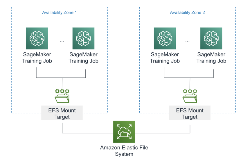
Figure 5-13. Amazon Elastic File System (EFS) with SageMaker

Data stored in EFS is replicated across multiple availability zones which provides higher availability and read/write throughput. The EFS file system will scale out automatically as new data is ingested.

Assuming you have mounted and populated the EFS file system with training data, you can pass the EFS mount into the training job using two(2) different implementations: FileSystemInput and FileSystemRecordSet.

This example shows how to use the FileSystemInput implementation:

estimator = TensorFlow(entry_point='tf_bert_reviews.py', 
                       source_dir='src', 
                       train_instance_count=train_instance_count,
                       train_instance_type=train_instance_type,
                       subnets=['subnet-1', 'subnet-2']
                       security_group_ids=['sg-1'])
efs_data = FileSystemInput(file_system_id='fs-1',
        			     file_system_type='EFS',
                           directory_path='/mnt/data,
                           file_system_access_mode='ro')
estimator.fit(inputs=efs_data)

Shard the Data with ShardedByS3Key

When training at scale, we need to consider how each instance in the cluster will read the large training datasets. We can use a brute-force approach and copy all of the data to all of the instances. However, with larger datasets, this may take a long time and potentially dominate the overall training time. For example, after performing feature engineering, our tokenized training dataset has approximately 45 TFRecord “part” files as shown below.

part-algo-1-amazon_reviews_us_Apparel_v1_00.tfrecord
...
part-algo-2-amazon_reviews_us_Digital_Software_v1_00.tfrecord
part-algo-4-amazon_reviews_us_Digital_Video_Games_v1_00.tfrecord
...
part-algo-9-amazon_reviews_us_Sports_v1_00.tfrecord

Rather than load all 45 parts files onto all instances in the cluster, we can improve startup performance by placing only 15 part files onto each of the 3 cluster instances for a total of 45 part files spread across the cluster. This is called “sharding.” We will use a SageMaker feature called ShardedByS3Key which evenly distributes the part files across the cluster as shown in Figure 5-14.

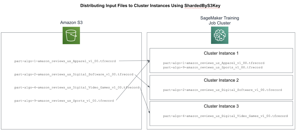
Figure 5-14. : Using ShardedByS3Key Distribution Strategy to Distribute the Input Files Across the Cluster Instances

Here we set up the ShardedByS3Key distribution strategy for our S3 input data including the train, validation, and test datasets:

s3_input_train_data = 
sagemaker.s3_input(s3_data=processed_train_data_s3_uri, 
         		  	   distribution='ShardedByS3Key') 
s3_input_validation_data =
sagemaker.s3_input(s3_data=processed_validation_data_s3_uri, 
   distribution='ShardedByS3Key')
s3_input_test_data = 
sagemaker.s3_input(s3_data=processed_test_data_s3_uri,                 
   distribution='ShardedByS3Key')

Next, we call fit() with the input map for each of our dataset splits including train, validation, and test.

estimator.fit(inputs={'train': s3_input_train_data, 
                      'validation': s3_input_validation_data,
                      'test': s3_input_test_data
              })

In this case, each instance in our cluster will receive approximately 15 files for each of the dataset splits.

Stream Data On-the-Fly with PipeMode

In addition to sharding, you can also use a SageMaker feature called PipeMode to load the data on-the-fly and as needed. Up until now, we’ve been using the default input_mode of File which copies all of the data to all the instances when the training job starts. This creates a long pause at the start of the training job as the data is copied.

PipeMode streams data in parallel from S3 directly into the training processes running on each instance which provides significantly-higher I/O throughput than File mode. All of this allows your training jobs to start quicker, complete faster, and use less disk space - lowering overall cost of your training and tuning jobs.

PipeMode works with S3 to pull the rows of training data as needed. Under the hood, PipeMode is using Unix first-in, first-out (FIFO) files to read data from S3 and cache it locally on the instance shortly before the data is needed by the training job. These FIFO files are one-way readable. In other words, you can’t back up or skip ahead randomly.

Here is how we configure our training job to use PipeMode:

input_mode='Pipe'
estimator = TensorFlow(entry_point='tf_bert_reviews.py', 
                       source_dir='src', 
                       train_instance_count=train_instance_count, 
                       train_instance_type=train_instance_type,

...

                       input_mode=input_mode)

Since PipeMode wraps our TensorFlow Dataset Reader, we need to change our TensorFlow code slightly to detect PipeMode and use the PipeModeDataset wrapper:

    if input_mode == 'Pipe':
        from sagemaker_tensorflow import PipeModeDataset
        dataset = PipeModeDataset(channel=channel,
                                  record_format='TFRecord')
    else:
        dataset = tf.data.TFRecordDataset(input_filenames)

Enable Enhanced Networking

Training at scale requires super-fast communication between instances in the cluster. Be sure to select an instance type that utilizes the enhanced networking adapter (ENA) and Elastic Fabric Adapter (EFA) to provide high network bandwidth and consistent network latency between the cluster instances.

The Enhanced Network Adapter (ENA) works well with the AWS deep learning instances types including the C, M, P, and X series. These instance types offer a large number of CPUs, so they benefit greatly from efficient sharing of the network adapter. By performing various network-level optimizations such as hardware-based checksum generation and software-based routing, ENA reduces overhead, improves scalability, and maximizes consistency. All of these optimizations are designed to reduce bottlenecks, offload work from the CPUs, and create an efficient path for the network packets.

The Elastic Fabric Adapter (EFA) uses custom-built, OS-level bypass techniques to improve network performance between instances in a cluster. EFA natively supports Message Passing Interface (MPI) which is critical to scaling high-performance computing (HPC) applications that scale to thousands of CPUs. EFA is supported by many of the compute-optimized instance types including the C and P series.