2. Human and Machine Language
In Chapter 1, we introduced the high-level theory of deep learning via analogy to the biological visual system. All the while, we highlighted that one of the technique’s core strengths lies in its ability to learn features automatically from data. In this chapter, we build atop our deep learning foundations by examining how deep learning is incorporated into human language applications, with a particular emphasis on how it can automatically learn features that represent the meaning of words.
The Austro-British philosopher Ludwig Wittgenstein famously argued, in his posthumous and seminal work Philosophical Investigations, “The meaning of a word is its use in the language.”1 He further wrote, “One cannot guess how a word functions. One has to look at its use, and learn from that.” Wittgenstein was suggesting that words on their own have no real meaning; rather, it is by their use within the larger context of that language that we’re able to ascertain their meaning. As you’ll see through this chapter, natural language processing with deep learning relies heavily on this premise. Indeed, the word2vec technique we introduce for converting words into numeric model inputs explicitly derives its semantic representation of a word by analyzing it within its contexts across a large body of language.
1. Wittgenstein, L. (1953). Philosophical Investigations. (Anscombe, G., Trans.). Oxford, UK: Basil Blackwell.
Armed with this notion, we begin by breaking down deep learning for natural language processing (NLP) as a discipline, and then we go on to discuss modern deep learning techniques for representing words and language. By the end of the chapter, you should have a good grasp on what is possible with deep learning and NLP, the groundwork for writing such code in Chapter 11.
Deep Learning for Natural Language Processing
The two core concepts in this chapter are deep learning and natural language processing. Initially, we cover the relevant aspects of these concepts separately, and then we weave them together as the chapter progresses.
Deep Learning Networks Learn Representations Automatically
As established way back in this book’s Preface, deep learning can be defined as the layering of simple algorithms called artificial neurons into networks several layers deep. Via the Venn diagram in Figure 2.1, we show how deep learning resides within the machine learning family of representation learning approaches. The representation learning family, which contemporary deep learning dominates, includes any techniques that learn features from data automatically. Indeed, we can use the terms “feature” and “representation” interchangeably.

Figure 2.1 Venn diagram that distinguishes the traditional family from the representation learning family of machine learning techniques
Figure 1.12 lays the foundation for understanding the advantage of representation learning relative to traditional machine learning approaches. Traditional ML typically works well because of clever, human-designed code that transforms raw data—whether it be images, audio of speech, or text from documents—into input features for machine learning algorithms (e.g., regression, random forest, or support vector machines) that are adept at weighting features but not particularly good at learning features from raw data directly. This manual creation of features is often a highly specialized task. For working with language data, for example, it might require graduate-level training in linguistics.
A primary benefit of deep learning is that it eases this requirement for subject-matter expertise. Instead of manually curating input features from raw data, one can feed the data directly into a deep learning model. Over the course of many examples provided to the deep learning model, the artificial neurons of the first layer of the network learn how to represent simple abstractions of these data, while each successive layer learns to represent increasingly complex nonlinear abstractions on the layer that precedes it. As you’ll discover in this chapter, this isn’t solely a matter of convenience; learning features automatically has additional advantages. Features engineered by humans tend to not be comprehensive, tend to be excessively specific, and can involve lengthy, ongoing loops of feature ideation, design, and validation that could stretch for years. Representation learning models, meanwhile, generate features quickly (typically over hours or days of model training), adapt straightforwardly to changes in the data (e.g., new words, meanings, or ways of using language), and adapt automatically to shifts in the problem being solved.
Natural Language Processing
Natural language processing is a field of research that sits at the intersection of computer science, linguistics, and artificial intelligence (Figure 2.2). NLP involves taking the naturally spoken or naturally written language of humans—such as this sentence you’re reading right now—and processing it with machines to automatically complete some task or to make a task easier for a human to do. Examples of language use that do not fall under the umbrella of natural language could include code written in a software language or short strings of characters within a spreadsheet.
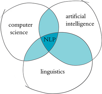
Figure 2.2 NLP sits at the intersection of the fields of computer science, linguistics, and artificial intelligence.
Examples of NLP in industry include:
Classifying documents: using the language within a document (e.g., an email, a Tweet, or a review of a film) to classify it into a particular category (e.g., high urgency, positive sentiment, or predicted direction of the price of a company’s stock).
Machine translation: assisting language-translation firms with machine-generated suggestions from a source language (e.g., English) to a target language (e.g., German or Mandarin); increasingly, fully automatic—though not always perfect—translations between languages.
Search engines: autocompleting users’ searches and predicting what information or website they’re seeking.
Speech recognition: interpreting voice commands to provide information or take action, as with virtual assistants like Amazon’s Alexa, Apple’s Siri, or Microsoft’s Cortana.
Chatbots: carrying out a natural conversation for an extended period of time; though this is seldom done convincingly today, they are nevertheless helpful for relatively linear conversations on narrow topics such as the routine components of a firm’s customer-service phone calls.
Some of the easiest NLP applications to build are spell checkers, synonym suggesters, and keyword-search querying tools. These simple tasks can be fairly straightforwardly solved with deterministic, rules-based code using, say, reference dictionaries or thesauruses. Deep learning models are unnecessarily sophisticated for these applications, and so they aren’t discussed further in this book.
Intermediate-complexity NLP tasks include assigning a school-grade reading level to a document, predicting the most likely next words while making a query in a search engine, classifying documents (see earlier list), and extracting information like prices or named entities2 from documents or websites. These intermediate NLP applications are well suited to solving with deep learning models. In Chapter 11, for example, you’ll leverage a variety of deep learning architectures to predict the sentiment of film reviews.
![]()
2. Named entities include places, well-known individuals, company names, and products.
The most sophisticated NLP implementations are required for machine translation (see earlier list), automated question-answering, and chatbots. These are tricky because they need to handle application-critical nuance (as an example, humor is particularly transient), a response to a question can depend on the intermediate responses to previous questions, and meaning can be conveyed over the course of a lengthy passage of text consisting of many sentences. Complex NLP tasks like these are beyond the scope of this book; however, the content we cover will serve as a superb foundation for their development.
A Brief History of Deep Learning for NLP
The timeline in Figure 2.3 calls out recent milestones in the application of deep learning to NLP. This timeline begins in 2011, when the University of Toronto computer scientist George Dahl and his colleagues at Microsoft Research revealed the first major breakthrough involving a deep learning algorithm applied to a large dataset.3 This breakthrough happened to involve natural language data. Dahl and his team trained a deep neural network to recognize a substantial vocabulary of words from audio recordings of human speech. A year later, and as detailed already in Chapter 1, the next landmark deep learning feat also came out of Toronto: AlexNet blowing the traditional machine learning competition out of the water in the ImageNet Large Scale Visual Recognition Challenge (Figure 1.15). For a time, this staggering machine vision performance heralded a focus on applying deep learning to machine vision applications.
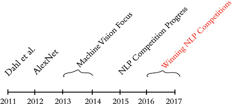
Figure 2.3 Milestones involving the application of deep learning to natural language processing
3. Dahl, G., et al. (2011). Large vocabulary continuous speech recognition with context-dependent DBN-HMMs. Proceedings of the International Conference on Acoustics, Speech, and Signal Processing.
By 2015, the deep learning progress being made in machine vision began to spill over into NLP competitions such as those that assess the accuracy of machine translations from one language into another. These deep learning models approached the precision of traditional machine learning approaches; however, they required less research and development time while conveniently offering lower computational complexity. Indeed, this reduction in computational complexity provided Microsoft the opportunity to squeeze real-time machine translation software onto mobile phone processors—remarkable progress for a task that previously had required an Internet connection and computationally expensive calculations on a remote server. In 2016 and 2017, deep learning models entered into NLP competitions not only were more efficient than traditional machine learning models, but they also began outperforming them on accuracy. The remainder of this chapter starts to illuminate how.
Computational Representations of Language
In order for deep learning models to process language, we have to supply that language to the model in a way that it can digest. For all computer systems, this means a quantitative representation of language, such as a two-dimensional matrix of numerical values. Two popular methods for converting text into numbers are one-hot encoding and word vectors.4 We discuss both methods in turn in this section.
4. If this were a book dedicated to NLP, then we would have been wise to also describe natural language methods based on word frequency, e.g., TF-IDF (term frequency-inverse document frequency) and PMI (pointwise mutual information).
One-Hot Representations of Words
The traditional approach to encoding natural language numerically for processing it with a machine is one-hot encoding (Figure 2.4). In this approach, the words of natural language in a sentence (e.g., “the,” “bat,” “sat,” “on,” “the,” and “cat”) are represented by the columns of a matrix. Each row in the matrix, meanwhile, represents a unique word. If there are 100 unique words across the corpus5 of documents you’re feeding into your natural language algorithm, then your matrix of one-hot-encoded words will have 100 rows. If there are 1,000 unique words across your corpus, then there will be 1,000 rows in your one-hot matrix, and so on.

Figure 2.4 One-hot encodings of words, such as this example, predominate the traditional machine learning approach to natural language processing.
![]()
5. A corpus (from the Latin “body”) is the collection of all of the documents (the “body” of language) you use as your input data for a given natural language application. In Chapter 11, you’ll make use of a corpus that consists of 18 classic books. Later in that chapter, you’ll separately make use of a corpus of 25,000 film reviews. An example of a much larger corpus would be all of the English-language articles on Wikipedia. The largest corpuses are crawls of all the publicly available data on the Internet, such as at commoncrawl.org.
Cells within one-hot matrices consist of binary values, that is, they are a 0 or a 1. Each column contains at most a single 1, but is otherwise made up of 0s, meaning that one-hot matrices are sparse.6 Values of one indicate the presence of a particular word (row) at a particular position (column) within the corpus. In Figure 2.4, our entire corpus has only six words, five of which are unique. Given this, a one-hot representation of the words in our corpus has six columns and five rows. The first unique word—the—occurs in the first and fifth positions, as indicated by the cells containing 1s in the first row of the matrix. The second unique word in our wee corpus is bat, which occurs only in the second position, so it is represented by a value of 1 in the second row of the second column. One-hot word representations like this are fairly straightforward, and they are an acceptable format for feeding into a deep learning model (or, indeed, other machine learning models). As you will see momentarily, however, the simplicity and sparsity of one-hot representations are limiting when incorporated into a natural language application.
6. Nonzero values are rare (i.e., they are sparse) within a sparse matrix. In contrast, dense matrices are rich in information: They typically contain few—perhaps even no—zero values.
Word Vectors
Vector representations of words are the information-dense alternative to one-hot encodings of words. Whereas one-hot representations capture information about word location only, word vectors (also known as word embeddings or vector-space embeddings) capture information about word meaning as well as location.7 This additional information renders word vectors favorable for a variety of reasons that are catalogued over the course of this chapter. The key advantage, however, is that—analogous to the visual features learned automatically by deep learning machine vision models in Chapter 1—word vectors enable deep learning NLP models to automatically learn linguistic features.
7. Strictly speaking, a one-hot representation is technically a “word vector” itself, because each column in a one-hot word matrix consists of a vector representing a word at a given location. In the deep learning community, however, use of the term “word vector” is commonly reserved for the dense representations covered in this section—that is, those derived by word2vec, GloVe, and related techniques.
When we’re creating word vectors, the overarching concept is that we’d like to assign each word within a corpus to a particular, meaningful location within a multidimensional space called the vector space. Initially, each word is assigned to a random location within the vector space. By considering the words that tend to be used around a given word within the natural language of your corpus, however, the locations of the words within the vector space can gradually be shifted into locations that represent the meaning of the words.8
8. As mentioned at the beginning of this chapter, this understanding of the meaning of a word from the words around it was proposed by Ludwig Wittgenstein. Later, in 1957, the idea was captured succinctly by the British linguist J.R. Firth with his phrase, “You shall know a word by the company it keeps.” Firth, J. (1957). Studies in linguistic analysis. Oxford: Blackwell.
Figure 2.5 uses a toy-sized example to demonstrate in more detail the mechanics behind the way word vectors are constructed. Commencing at the first word in our corpus and moving to the right one word at a time until we reach the final word in our corpus, we consider each word to be the target word. At the particular moment captured in Figure 2.5, the target word that happens to be under consideration is word. The next target word would be by, followed by the, then company, and so on. For each target word in turn, we consider it relative to the words around it—its context words. In our toy example, we’re using a context-word window size of three words. This means that while word is the target word, the three words to the left (a, know, and shall) combined with the three words to the right (by, company, and the) together constitute a total of six context words.9 When we move along to the subsequent target word (by), the windows of context words also shift one position to the right, dropping shall and by as context words while adding word and it.
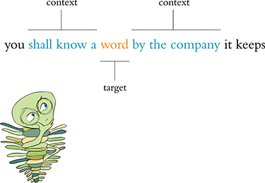
Figure 2.5 A toy-sized example for demonstrating the high-level process behind techniques like word2vec and GloVe that convert natural language into word vectors
9. It is mathematically simpler and more efficient to not concern ourselves with the specific ordering of context words, particularly because word order tends to confer negligible extra information to the inference of word vectors. Ergo, we provide the context words in parentheses alphabetically, an effectively random order.
Two of the most popular techniques for converting natural language into word vectors are word2vec10 and GloVe.11 With either technique, our objective while considering any given target word is to accurately predict the target word given its context words.12 Improving at these predictions, target word after target word over a large corpus, we gradually assign words that tend to appear in similar contexts to similar locations in vector space.
10. Mikolov, T., et al. (2013). Efficient estimation of word representations in vector space. arXiv:1301.3781.
11. Pennington, J., et al. (2014). GloVe: Global vectors for word representations. Proceedings of the Conference on Empirical Methods in Natural Language Processing.
12. Or, alternatively, we could predict context words given a target word. More on that in Chapter 11.
Figure 2.6 provides a cartoon of vector space. The space can have any number of dimensions, so we can call it an n-dimensional vector space. In practice, depending on the richness of the corpus we have to work with and the complexity of our NLP application, we might create a word-vector space with dozens, hundreds, or—in extreme cases—thousands of dimensions. As overviewed in the previous paragraph, any given word from our corpus (e.g., king) is assigned a location within the vector space. In, say, a 100-dimensional space, the location of the word king is specified by a vector that we can call υking that must consist of 100 numbers in order to specify the location of the word king across all of the available dimensions.
Human brains aren’t adept at spatial reasoning in more than three dimensions, so our cartoon in Figure 2.6 has only three dimensions. In this three-dimensional space, any given word from our corpus needs three numeric coordinates to define its location within the vector space: x, y, and z. In this cartoon example, then, the meaning of the word king is represented by a vector υking that consists of three numbers. If υking is located at the coordinates x = –0.9, y = 1.9, and z = 2.2 in the vector space, we can use the annotation [-0.9, 1.9, 2.2] to describe this location succinctly. This succinct annotation will come in handy shortly when we perform arithmetic operations on word vectors.
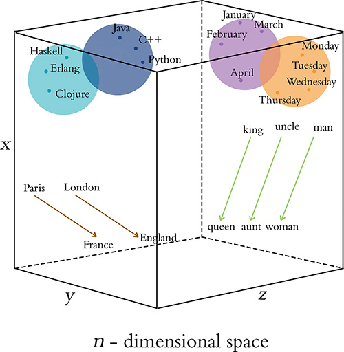
Figure 2.6 Diagram of word meaning as represented by a three-dimensional vector space
The closer two words are within vector space,13 the closer their meaning, as determined by the similarity of the context words appearing near them in natural language. Synonyms and common misspellings of a given word—because they share an identical meaning—would be expected to have nearly identical context words and therefore nearly identical locations in vector space. Words that are used in similar contexts, such as those that denote time, tend to occur near each other in vector space. In Figure 2.6, Monday, Tuesday, and Wednesday could be represented by the orange-colored dots located within the orange days-of-the-week cluster in the cube’s top-right corner. Meanwhile, months of the year might occur in their own purple cluster, which is adjacent to, but distinct from, the days of the week; they both relate to the date, but they’re separate subclusters within a broader dates region. As a second example, we would expect to find programming languages clustering together in some location within the word-vector space that is distant from the time-denoting words—say, in the top-left corner. Again here, object-oriented programming languages like Java, C++, and Python would be expected to form one subcluster, while nearby we would expect to find functional programming languages like Haskell, Clojure, and Erlang forming a separate subcluster. As you’ll see in Chapter 11 when you embed words in vector space yourself, less concretely defined terms that nevertheless convey a specific meaning (e.g., the verbs created, developed, and built) are also allocated positions within word-vector space that enable them to be useful in NLP tasks.
13. Measured by Euclidean distance, which is the plain old straight-line distance between two points.
Word-Vector Arithmetic
Remarkably, because particular movements across vector space turn out to be an efficient way for relevant word information to be stored in the vector space, these movements come to represent relative particular meanings between words. This is a bewildering property.14 Returning to our cube in Figure 2.6, the brown arrows represent the relationship between countries and their capitals. That is, if we calculate the direction and distance between the coordinates of the words Paris and France and then trace this direction and distance from London, we should find ourselves in the neighborhood of the coordinate representing the word England. As a second example, we can calculate the direction and distance between the coordinates for man and woman. This movement through vector space represents gender and is symbolized by the green arrows in Figure 2.6. If we trace the green direction and distance from any given male-specific term (e.g., king, uncle), we should find our way to a coordinate near the term’s female-specific counterpart (queen, aunt).
14. One of your esteemed authors, Jon, prefers terms like “mind-bending” and “trippy” to describe this property of word vectors, but he consulted a thesaurus to narrow in on a more professional-sounding adjective.
A by-product of being able to trace vectors of meaning (e.g., gender, capital-country relationship) from one word in vector space to another is that we can perform word-vector arithmetic. The canonical example of this is as follows: If we begin at υking, the vector representing king (continuing with our example from the preceding section, this location is described by [-0.9, 1.9, 2.2]), subtract the vector representing man from it (let’s say υman = [-1.1, 2.4, 3.0]), and add the vector representing woman (let’s say υwoman = [-3.2, 2.5, 2.6]), we should find a location near the vector representing queen. To make this arithmetic explicit by working through it dimension by dimension, we would estimate the location of υqueen by calculating
All three dimensions together, then, we expect υqueen to be near [-3.0, 2.0, 1.8].
Figure 2.7 provides further, entertaining examples of arithmetic through a word-vector space that was trained on a large natural language corpus crawled from the web. As you’ll later observe in practice in Chapter 11, the preservation of these quantitative relationships of meaning between words across vector space is a robust starting point for deep learning models within NLP applications.

Figure 2.7 Examples of word-vector arithmetic
word2viz
To develop your intuitive appreciation of word vectors, navigate to bit.ly/word2viz. The default screen for the word2viz tool for exploring word vectors interactively is shown in Figure 2.8. Leaving the top-right dropdown box set to “Gender analogies,” try adding in pairs of new words under the “Modify words” heading. If you add pairs of corresponding gender-specific words like princess and prince, duchess and duke, and businesswoman and businessman, you should find that they fall into instructive locations.
The developer of the word2viz tool, Julia Bazińska, compressed a 50-dimensional word-vector space down to two dimensions in order to visualize the vectors on an xy-coordinate system.15 For the default configuration, Bazińska scaled the x-axis from the words she to he as a reference point for gender, while the y-axis was set to vary from a commonfolk base toward a royal peak by orienting it to the words woman and queen. The displayed words, placed into vector space via training on a natural language dataset consisting of 6 billion instances of 400,000 unique words,16 fall relative to the two axes based on their meaning. The more regal (queen-like) the words, the higher on the plot they should be shown, and the female (she-like) terms fall to the left of their male (he-like) counterparts.
15. We detail how to reduce the dimensionality of a vector space for visualization purposes in Chapter 11.
16. Technically, 400,000 tokens—a distinction that we examine later.
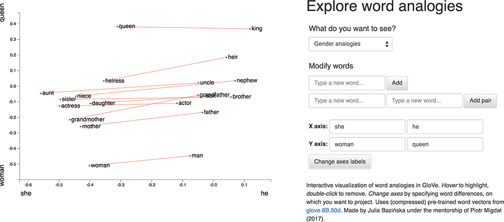
Figure 2.8 The default screen for word2viz, a tool for exploring word vectors interactively
When you’ve indulged yourself sufficiently with word2viz’s “Gender analogies” view, you can experiment with other perspectives of the word-vector space. Selecting “Adjectives analogies” from the “What do you want to see?” dropdown box, you could, for example, add the words small and smallest. Subsequently, you could change the x-axis labels to nice and nicer, and then again to small and big. Switching to the “Numbers say-write analogies” view via the dropdown box, you could play around with changing the x-axis to 3 and 7.
You may build your own word2viz plot from scratch by moving to the “Empty” view. The (word vector) world is your oyster, but you could perhaps examine the country-capital relationships we mentioned earlier when familiarizing you with Figure 2.6. To do this, set the x-axis to range from west to east and the y-axis to city and country. Word pairs that fall neatly into this plot include london—england, paris—france, berlin—germany and beijing—china.
Localist Versus Distributed Representations
With an intuitive understanding of word vectors under our figurative belts, we can contrast them with one-hot representations (Figure 2.4), which have been an established presence in the NLP world for longer. A summary distinction is that we can say word vectors store the meaning of words in a distributed representation across n-dimensional space. That is, with word vectors, word meaning is distributed gradually—smeared—as we move from location to location through vector space. One-hot representations, meanwhile, are localist. They store information on a given word discretely, within a single row of a typically extremely sparse matrix.
To more thoroughly characterize the distinction between the localist, one-hot approach and the distributed, vector-based approach to word representation, Table 2.1 compares them across a range of attributes. First, one-hot representations lack nuance; they are simple binary flags. Vector-based representations, on the other hand, are extremely nuanced: Within them, information about words is smeared throughout a continuous, quantitative space. In this high-dimensional space, there are essentially infinite possibilities for capturing the relationships between words.
Table 2.1 Contrasting attributes of localist, one-hot representations of words with distributed, vector-based representations
One-Hot |
Vector-Based |
|---|---|
Not subtle |
Very nuanced |
Manual taxonomies |
Automatic |
Handles new words poorly |
Seamlessly incorporates new words |
Subjective |
Driven by natural language data |
Word similarity not represented |
Word similarity = proximity in space |
Second, the use of one-hot representations in practice often requires labor-intensive, manually curated taxonomies. These taxonomies include dictionaries and other specialized reference language databases.18 Such external references are unnecessary for vector-based representations, which are fully automatic with natural language data alone.
18. For example, WordNet (wordnet.princeton.edu), which describes synonyms as well as hypernyms (“is-a” relationships, so furniture, for example, is a hypernym of chair).
Third, one-hot representations don’t handle new words well. A newly introduced word requires a new row in the matrix and then reanalysis relative to the existing rows of the corpus, followed by code changes—perhaps via reference to external information sources. With vector-based representations, new words can be incorporated by training the vector space on natural language that includes examples of the new words in their natural context. A new word gets its own new n-dimensional vector. Initially, there may be few training data points involving the new word, so its vector might not be very accurately positioned within n-dimensional space, but the positioning of all existing words remains intact and the model will not fail to function. Over time, as the instances of the new word in natural language increases, the accuracy of its vector-space coordinates will improve.19
19. An associated problem not addressed here occurs when an in-production NLP algorithm encounters a word that was not included within its corpus of training data. This out of vocabulary problem impacts both one-hot representations and word vectors. There are approaches—such as Facebook’s fastText library—that try to get around the issue by considering subword information, but these approaches are beyond the scope of this book.
Fourth, and following from the previous two points, the use of one-hot representations often involves subjective interpretations of the meaning of language. This is because they often require coded rules or reference databases that are designed by (relatively small groups of) developers. The meaning of language in vector-based representations, meanwhile, is data driven.20
20. Noting that they may nevertheless include biases found in natural language data. See the sidebar beginning on page 31.
Fifth, one-hot representations natively ignore word similarity: Similar words, such as couch and sofa, are represented no differently than unrelated words, such as couch and cat. In contrast, vector-based representations innately handle word similarity: As mentioned earlier with respect to Figure 2.6, the more similar two words are, the closer they are in vector space.
Elements of Natural Human Language
Thus far, we have considered only one element of natural human language: the word. Words, however, are made up of constituent language elements. In turn, words themselves are the constituents of more abstract, more complex language elements. We begin with the language elements that make up words and build up from there, following the schematic in Figure 2.9. With each element, we discuss how it is typically encoded from the traditional machine learning perspective as well as from the deep learning perspective. As we move through these elements, notice that the distributed deep learning representations are fluid and flexible vectors whereas the traditional ML representations are local and rigid (Table 2.2).
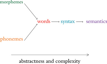
Figure 2.9 Relationships between the elements of natural human language. The leftmost elements are building blocks for further-right elements. As we move to the right, the more abstract the elements become, and therefore the more complex they are to model within an NLP application.
Table 2.2 Traditional machine learning and deep learning representations, by natural language element
Representation |
Traditional ML |
Deep Learning |
Audio-Only |
|---|---|---|---|
Phonology |
All phonemes |
Vectors |
True |
Morphology |
All morphemes |
Vectors |
False |
Words |
One-hot encoding |
Vectors |
False |
Syntax |
Phrase rules |
Vectors |
False |
Semantics |
Lambda calculus |
Vectors |
False |
Phonology is concerned with the way that language sounds when it is spoken. Every language has a specific set of phonemes (sounds) that make up its words. The traditional ML approach is to encode segments of auditory input as specific phonemes from the language’s range of available phonemes. With deep learning, we train a model to predict phonemes from features automatically learned from auditory input and then represent those phonemes in a vector space. In this book, we work with natural language in text format only, but the techniques we cover can be applied directly to speech data if you’re keen to do so on your own time.
Morphology is concerned with the forms of words. Like phonemes, every language has a specific set of morphemes, which are the smallest units of language that contain some meaning. For example, the three morphemes out, go, and ing combine to form the word outgoing. The traditional ML approach is to identify morphemes in text from a list of all the morphemes in a given language. With deep learning, we train a model to predict the occurrence of particular morphemes. Hierarchically deeper layers of artificial neurons can then combine multiple vectors (e.g., the three representing out, go, and ing) into a single vector representing a word.
Phonemes (when considering audio) and morphemes (when considering text) combine to form words. Whenever we work with natural language data in this book, we work at the word level. We do this for four reasons. First, it’s straightforward to define what a word is, and everyone is familiar with what they are. Second, it’s easy to break up natural language into words via a process called tokenization21 that we work through in Chapter 11. Third, words are the most-studied level of natural language, particularly with respect to deep learning, so we can readily apply cutting-edge techniques to them. Fourth, and perhaps most critically, for the NLP models we’ll be building, word vectors simply work well: They prove to be functional, efficient, and accurate. In the preceding section, we detail the shortcomings of localist, one-hot representations that predominate traditional ML relative to the word vectors used in deep learning models.
21. Essentially, tokenization is the use of characters like commas, periods, and whitespace to assume where one word ends and the next begins.
Words are combined to generate syntax. Syntax and morphology together constitute the entirety of a language’s grammar. Syntax is the arrangement of words into phrases and phrases into sentences in order to convey meaning in a way that is consistent across the users of a given language. In the traditional ML approach, phrases are bucketed into discrete, formal linguistic categories.22 With deep learning, we employ vectors (surprise, surprise!). Every word and every phrase in a section of text can be represented by a vector in n-dimensional space, with layers of artificial neurons combining words into phrases.
22. These categories have names like “noun-phrase” and “verb-phrase.”
Semantics is the most abstract of the elements of natural language in Figure 2.9 and Table 2.2; it is concerned with the meaning of sentences. This meaning is inferred from all the underlying language elements like words and phrases, as well as the overarching context that a piece of text appears in. Inferring meaning is complex because, for example, whether a passage is supposed to be taken literally or as a humorous and sarcastic remark can depend on subtle contextual differences and shifting cultural norms. Traditional ML, because it doesn’t represent the fuzziness of language (e.g., the similarity of related words or phrases), is limited in capturing semantic meaning. With deep learning, vectors come to the rescue once again. Vectors can represent not only every word and every phrase in a passage of text but also every logical expression. As with the language elements already covered, layers of artificial neurons can recombine vectors of constituent elements—in this case, to calculate semantic vectors via the nonlinear combination of phrase vectors.
Google Duplex
One of the more attention-grabbing examples of deep-learning-based NLP in recent years is that of the Google Duplex technology, which was unveiled at the company’s I/O developers conference in May 2018. The search giant’s CEO, Sundar Pichai, held spectators in rapture as he demonstrated Google Assistant making a phone call to a Chinese-food restaurant to book a reservation. The audible gasps from the audience were in response to the natural flow of Duplex’s conversation. It had mastered the cadence of a human conversation, replete with the uh’s and hhhm’s that we sprinkle into conversations while we’re thinking. Furthermore, the phone call was of average audio quality and the human on the line had a strong accent; Duplex never faltered, and it managed to make the booking.
Bearing in mind that this is a demonstration—and not even a live one—what nevertheless impressed us was the breadth of deep learning applications that had to come together to facilitate this technology. Consider the flow of information back and forth between the two agents on the call (Duplex and the restaurateur): Duplex needs a sophisticated speech recognition algorithm that can process audio in real time and handle an extensive range of accents and call qualities on the other end of the line, and also overcome the background noise.23
23. This is known as the “cocktail-party problem”—or less jovially, “multitalker speech separation.” It’s a problem that humans solve innately, isolating single voices from a cacophony quite well without explicit instruction on how to do so. Machines typically struggle with this, although a variety of groups have proposed solutions. For example, see Simpson, A., et al. (2015). Deep karaoke: Extracting vocals from musical mixtures using a convolutional deep neural network. arXiv:1504.04658; Yu, D., et al. (2016). Permutation invariant training of deep models for speaker-independent multi-talker speech separation. arXiv:1607.00325.
Once the human’s speech has been faithfully transcribed, an NLP model needs to process the sentence and decide what it means. The intention is that the person on the line doesn’t know they’re speaking to a computer and so doesn’t need to modulate their speech accordingly, but in turn, this means that humans respond with complex, multipart sentences that can be tricky for a computer to tease apart:
“We don’t have anything tomorrow, but we have the next day and Thursday, anytime before eight. Wait no . . . Thursday at seven is out. But we can do it after eight?”
This sentence is poorly structured—you’d never write an email like this—but in natural conversation, these sorts of on-the-fly corrections and replacements happen regularly, and Duplex needs to be able to follow along.
With the audio transcribed and the meaning of the sentence processed, Duplex’s NLP model conjures up a response. This response must ask for more information if the human was unclear or if the answers were unsatisfactory; otherwise, it should confirm the booking. The NLP model will generate a response in text form, so a text-to-speech (TTS) engine is required to synthesize the sound.
To misquote Jerry Maguire, you had all of this at “hello.” The speech recognition system, NLP models, and TTS engine all work in concert from the instant the call is answered. Things only stand to get more complex for Duplex from then on. Governing all of this interaction is a deep neural network that is specialized in handling information that occurs in a sequence.28 This governor tracks the conversation and feeds the various inputs and outputs into the appropriate models.
28. Called a recurrent neural network. These feature in Chapter 11.
It should be clear from this overview that Google Duplex is a sophisticated system of deep learning models that work in harmony to produce a seamless interaction on the phone. For now, Duplex is nevertheless limited to a few specific domains: scheduling appointments and reservations. The system cannot carry out general conversations. So even though Duplex represents a significant step forward for artificial intelligence, there is still much work to be done.
Summary
In this chapter, you learned about applications of deep learning to the processing of natural language. To that end, we described further the capacity for deep learning models to automatically extract the most pertinent features from data, removing the need for labor-intensive one-hot representations of language. Instead, NLP applications involving deep learning make use of vector-space embeddings, which capture the meaning of words in a nuanced manner that improves both model performance and accuracy.
In Chapter 11, you’ll construct an NLP application by making use of artificial neural networks that handle the input of natural language data all the way through to the output of an inference about those data. In such “end-to-end” deep learning models, the initial layers create word vectors that flow seamlessly into deeper, specialized layers of artificial neurons, including layers that incorporate “memory.” These model architectures highlight both the strength and the ease of use of deep learning with word vectors.
