6. Artificial Neurons Detecting Hot Dogs
Having received tantalizing exposure to applications of deep learning in the first part of this book and having coded up a functioning neural network in Chapter 5, the moment has come to delve into the nitty-gritty theory underlying these capabilities. We begin by dissecting artificial neurons, the units that—when wired together—constitute an artificial neural network.
Biological Neuroanatomy 101
As presented in the opening paragraphs of this book, ersatz neurons are inspired by biological ones. Given that, let’s take a gander at Figure 6.1 for a précis of the first lecture in any neuroanatomy course: A given biological neuron receives input into its cell body from many (generally thousands) of dendrites, with each dendrite receiving signals of information from another neuron in the nervous system—a biological neural network. When the signal conveyed along a dendrite reaches the cell body, it causes a small change in the voltage of the cell body.1 Some dendrites cause a small positive change in voltage, and the others cause a small negative change. If the cumulative effect of these changes causes the voltage to increase from its resting state of –70 millivolts to the critical threshold of –55 millivolts, the neuron will fire something called an action potential away from its cell body, down its axon, thereby transmitting a signal to other neurons in the network.

Figure 6.1 The anatomy of a biological neuron
1. More precisely, it causes a change in the voltage difference between the cell’s interior and its surroundings.
To summarize, biological neurons exhibit the following three behaviors in sequence:
Receive information from many other neurons
Aggregate this information via changes in cell voltage at the cell body
Transmit a signal if the cell voltage crosses a threshold level, a signal that can be received by many other neurons in the network
The Perceptron
In the late 1950s, the American neurobiologist Frank Rosenblatt (Figure 6.2) published an article on his perceptron, an algorithm influenced by his understanding of biological neurons, making it the earliest formulation of an artificial neuron.2 Analogous to its living inspiration, the perceptron (Figure 6.3) can:
Receive input from multiple other neurons
Aggregate those inputs via a simple arithmetic operation called the weighted sum
Generate an output if this weighted sum crosses a threshold level, which can then be sent on to many other neurons within a network

Figure 6.2 The American neurobiology and behavior researcher Frank Rosenblatt. He conducted much of his work out of the Cornell Aeronautical Laboratory, including physically constructing his Mark I Perceptron there. This machine, an early relic of artificial intelligence, can today be viewed at the Smithsonian Institution in Washington, D.C.
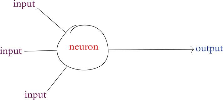
Figure 6.3 Schematic diagram of a perceptron, an early artificial neuron. Note the structural similarity to the biological neuron in Figure 6.1.
2. Rosenblatt, F. (1958). The perceptron: A probabilistic model for information storage and the organization in the brain. Psychological Review, 65, 386–408.
The Hot Dog / Not Hot Dog Detector
Let’s work through a lighthearted example to understand how the perceptron algorithm works. We’re going to look at a perceptron that is specialized in distinguishing whether a given object is a hot dog or, well . . . not a hot dog.
A critical attribute of perceptrons is that they can only be fed binary information as inputs, and their output is also restricted to being binary. Thus, our hot dog-detecting perceptron must be fed its particular three inputs (indicating whether the object involves ketchup, mustard, or a bun, respectively) as either a 0 or a 1. In Figure 6.4:
The first input (a purple 1) indicates the object being presented to the perceptron involves ketchup.
The second input (also a purple 1) indicates the object has mustard.
The third input (a purple 0) indicates the object does not include a bun.

Figure 6.4 First example of a hot dog-detecting perceptron: In this instance, it predicts there is indeed a hot dog.
To make a prediction as to whether the object is a hot dog or not, the perceptron independently weights each of these three inputs.3 The weights that we arbitrarily selected in this (entirely contrived) hot dog example indicate that the presence of a bun, with its weight of 6, is the most influential predictor of whether the object is a hot dog or not. The intermediate-weight predictor is ketchup with its weight of 3, and the least influential predictor is mustard, with a weight of 2.
3. If you are well accustomed to regression modeling, this should be a familiar paradigm.
Let’s determine the weighted sum of the inputs: One input at a time (i.e., elementwise), we multiply the input by its weight and then sum the individual results. So first, let’s calculate the weighted inputs:
For the ketchup input: 3 × 1 = 3
For mustard: 2 × 1 = 2
For bun: 6 × 0 = 0
With those three products, we can compute that the weighted sum of the inputs is 5: 3 + 2 + 0. To generalize from this example, the calculation of the weighted sum of inputs is:
Where:
wi is the weight of a given input i (in our example, w1 = 3, w2 = 2, and w3 = 6).
xi is the value of a given input i (in our example, x1 = 1, x2 = 1, and x3 = 0).
wixi represents the product of wi and xi—i.e., the weighted value of a given input i.
indicates that we sum all of the individual weighted inputs wixi, where n is the total number of inputs (in our example, we had three inputs, but artificial neurons can have any number of inputs).
The final step of the perceptron algorithm is to evaluate whether the weighted sum of the inputs is greater than the neuron’s threshold. As with the earlier weights, we have again arbitrarily chosen a threshold value for our perceptron example: 4 (shown in red in the center of the neuron in Figure 6.4). The perceptron algorithm is:
where
If the weighted sum of a perceptron’s inputs is greater than its threshold, then it outputs a
1, indicating that the perceptron predicts the object is a hot dog.If the weighted sum is less than or equal to the threshold, the perceptron outputs a
0, indicating that it predicts there is not a hot dog.
Knowing this, we can wrap up our example from Figure 6.4: The weighted sum of 5 is greater than the neuron’s threshold of 4, and so our hot dog-detecting perceptron outputs a 1.
Riffing on our first hot dog example, in Figure 6.5 the object evaluated by the perceptron now includes mustard only; there is no ketchup, and it is still without a bun. In this case the weighted sum of inputs comes out to 2. Because 2 is less than the perceptron’s threshold, the neuron outputs 0, indicating that it predicts this object is not a hot dog.

Figure 6.5 Second example of a hot dog-detecting perceptron: In this instance, it predicts there is not a hot dog.
In our third and final perceptron example, shown in Figure 6.6, the artificial neuron evaluates an object that involves neither mustard nor ketchup but is on a bun. The presence of a bun alone corresponds to the calculation of a weighted sum of 6. Because 6 is greater than the perceptron’s threshold, the algorithm predicts that the object is a hot dog and outputs a 1.
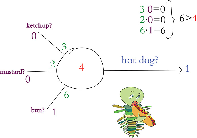
Figure 6.6 Third example of a hot dog-detecting perceptron: In this instance, it again predicts the object presented to it is a hot dog.
The Most Important Equation in This Book
To achieve the formulation of a simplified and universal perceptron equation, we must introduce a term called the bias, which we annotate as b and which is equivalent to the negative of an artificial neuron’s threshold value:
Together, a neuron’s bias and its weights constitute all of its parameters: the changeable variables that prescribe what the neuron will output in response to its inputs.
With the concept of a neuron’s bias now available to us, we arrive at the most widely used perceptron equation:
Notice that we made the following five updates to our initial perceptron equation (from Equation 6.2):
Substituted the bias b in place of the neuron’s threshold
Flipped b onto the same side of the equation as all of the other variables
Used the array w to represent all of the wi weights from w1 through to wn
Likewise, used the array x to represent all of the xi values from x1 through to xn
Used the dot product notation w · x to abbreviate the representation of the weighted sum of neuron inputs (the longer form of this is shown in Equation 6.1: )
Right at the heart of the perceptron equation in Equation 6.4 is w · x + b, which we have cut out for emphasis and placed alone in Figure 6.7. If there is one item you note down to remember from this chapter, it should be this three-variable formula, which is an equation that represents artificial neurons in general. We refer to this equation many times over the course of this book.
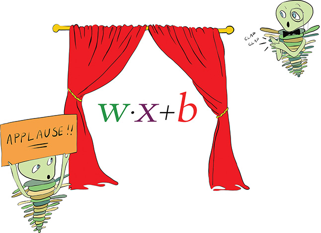
Figure 6.7 The general equation for artificial neurons that we will return to time and again. It is the most important equation in this book.
Modern Neurons and Activation Functions
Modern artificial neurons—such as those in the hidden layer of the shallow architecture we built in Chapter 5 (look back to Figure 5.4 or to our Shallow Net in Keras notebook)—are not perceptrons. While the perceptron provides a relatively uncomplicated introduction to artificial neurons, it is not used widely today. The most obvious restriction of the perceptron is that it receives only binary inputs, and provides only a binary output. In many cases, we’d like to make predictions from inputs that are continuous variables and not binary integers, and so this restriction alone would make perceptrons unsuitable.
A less obvious (yet even more critical) corollary of the perceptron’s binary-only restriction is that it makes learning rather challenging. Consider Figure 6.8, in which we use a new term, z, as shorthand for the value of the lauded w · x + b equation from Figure 6.7.

Figure 6.8 The perceptron’s transition from outputting zero to outputting one happens suddenly, making it challenging to gently tune w and b to match a desired output.
When z is any value less than or equal to zero, the perceptron outputs its smallest possible output, 0. If z becomes positive to even the tiniest extent, the perceptron outputs its largest possible output, 1. This sudden and extreme transition is not optimal during training: When we train a network, we make slight adjustments to w and b based on whether it appears the adjustment will improve the network’s output.4 With the perceptron, the majority of slight adjustments to w and b would make no difference whatsoever to its output; z would generally be moving around at negative values much lower than 0 or at positive values much higher than 0. That behavior on its own would be unhelpful, but the situation is even worse: Every once in a while, a slight adjustment to w or b will cause z to cross from negative to positive (or vice versa), leading to a whopping, drastic swing in output from 0 all the way to 1 (or vice versa). Essentially, the perceptron has no finesse—it’s either yelling or it’s silent.
4. Improve here means providing output more closely in line with the true output y given some input x. We discuss this further in Chapter 8.
The Sigmoid Neuron
Figure 6.9 provides an alternative to the erratic behavior of the perceptron: a gentle curve from 0 to 1. This particular curve shape is called the sigmoid function and is defined by , where:
z is equivalent to w · x + b.
e is the mathematical constant beginning in 2.718. It is perhaps best known for its starring role in the natural exponential function.
σ is the Greek letter sigma, the root word for “sigmoid.”
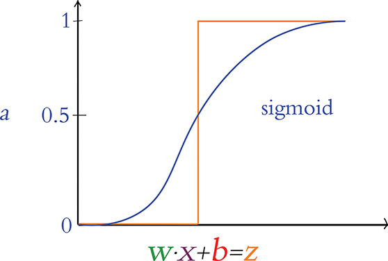
Figure 6.9 The sigmoid activation function
The sigmoid function is our first example of an artificial neuron activation function. It may be ringing a bell for you already, because it was the neuron type that we selected for the hidden layer of our Shallow Net in Keras from Chapter 5. As you’ll see as this section progresses, the sigmoid function is the canonical activation function—so much so that the Greek letter σ (sigma) is conventionally used to denote any activation function. The output from any given neuron’s activation function is referred to simply as its activation, and throughout this book, we use the variable term a—as shown along the vertical axis in Figure 6.9—to denote it.
In our view, there is no need to memorize the sigmoid function (or indeed any of the activation functions). Instead, we believe it’s easier to understand a given function by playing around with its behavior interactively. With that in mind, feel free to join us in the Sigmoid Function Jupyter notebook from the book’s GitHub repository as we work through the following lines of code.
Our only dependency in the notebook is the constant e, which we load using the statement from math import e. Next is the fun bit, where we define the sigmoid function itself:
def sigmoid(z):
    return 1/(1+e**-z)
As depicted in Figure 6.9 and demonstrated by executing sigmoid(.00001), near-0 inputs into the sigmoid function will lead it to return values near 0.5. Increasingly large positive inputs will result in values that approach 1. As an extreme example, an input of 10000 results in an output of 1.0. Moving more gradually with our inputs—this time in the negative direction—we obtain outputs that gently approach 0: As examples, sigmoid(-1) returns 0.2689, while sigmoid(-10) returns 4.5398e-05.5
5. The e in 4.5398e-05 should not be confused with the base of the natural logarithm. Used in code outputs, it refers to an exponent, so the output is the equivalent of 4.5398 × 10⁻⁵.
Any artificial neuron that features the sigmoid function as its activation function is called a sigmoid neuron, and the advantage of these over the perceptron should now be tangible: Small, gradual changes in a given sigmoid neuron’s parameters w or b cause small, gradual changes in z, thereby producing similarly gradual changes in the neuron’s activation, a. Large negative or large positive values of z illustrate an exception: At extreme z values, sigmoid neurons—like perceptrons—will output 0’s (when z is negative) or 1’s (when z is positive). As with the perceptron, this means that subtle updates to the weights and biases during training will have little to no effect on the output, and thus learning will stall. This situation is called neuron saturation and can occur with most activation functions. Thankfully, there are tricks to avoid saturation, as you’ll see in Chapter 9.
The Tanh Neuron
A popular cousin of the sigmoid neuron is the tanh (pronounced “tanch” in the deep learning community) neuron. The tanh activation function is pictured in Figure 6.10 and is defined by . The shape of the tanh curve is similar to the sigmoid curve, with the chief distinction being that the sigmoid function exists in the range [0 : 1], whereas the tanh neuron’s output has the range [–1 : 1]. This difference is more than cosmetic. With negative z inputs corresponding to negative a activations, z = 0 corresponding to a = 0, and positive z corresponding to positive a activations, the output from tanh neurons tends to be centered near 0. As we cover further in Chapters 7 through 9, these 0-centered a outputs usually serve as the inputs x to other artificial neurons in a network, and such 0-centered inputs make (the dreaded!) neuron saturation less likely, thereby enabling the entire network to learn more efficiently.
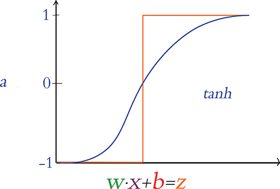
Figure 6.10 The tanh activation function
ReLU: Rectified Linear Units
The final neuron we detail in this book is the rectified linear unit, or ReLU neuron, whose behavior we graph in Figure 6.11. The ReLU activation function, whose shape diverges glaringly from the sigmoid and tanh sorts, was inspired by properties of biological neurons6 and popularized within artificial neural networks by Vinod Nair and Geoff Hinton (Figure 1.16).7 The shape of the ReLU function is defined by a = max(0, z).
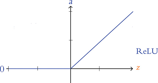
Figure 6.11 The ReLU activation function
6. The action potentials of biological neurons have only a “positive” firing mode; they have no “negative” firing mode. See Hahnloser, R., & Seung, H. (2000). Permitted and forbidden sets in symmetric threshold-linear networks. Advances in Neural Information Processing Systems, 13.
7. Nair, V., & Hinton, G. (2010). Rectified linear units improve restricted Boltzmann machines. Proceedings of the International Conference on Machine Learning.
This function is uncomplicated:
If z is a positive value, the ReLU activation function returns z (unadulterated) as a = z.
If z = 0 or z is negative, the function returns its floor value of 0, that is, the activation a = 0.
The ReLU function is one of the simplest functions to imagine that is nonlinear. That is, like the sigmoid and tanh functions, its output a does not vary uniformly linearly across all values of z. The ReLU is in essence two distinct linear functions combined (one at negative z values returning 0, and the other at positive z values returning z, as is visible in Figure 6.11) to form a straightforward, nonlinear function overall. This nonlinear nature is a critical property of all activation functions used within deep learning architectures. As demonstrated via a series of captivating interactive applets in Chapter 4 of Michael Nielsen’s Neural Networks and Deep Learning e-book, these nonlinearities permit deep learning models to approximate any continuous function.8 This universal ability to approximate some output y given some input x is one of the hallmarks of deep learning—the characteristic that makes the approach so effective across such a breadth of applications.
8. neuralnetworksanddeeplearning.com/chap4.html
The relatively simple shape of the ReLU function’s particular brand of nonlinearity works to its advantage. As you’ll see in Chapter 8, learning appropriate values for w and b within deep learning networks involves partial derivative calculus, and these calculus operations are more computationally efficient on the linear portions of the ReLU function relative to its efficiency on the curves of, say, the sigmoid and tanh functions.9 As a testament to its utility, the incorporation of ReLU neurons into AlexNet (Figure 1.17) was one of the factors behind its trampling of existing machine vision benchmarks in 2012 and shepherding in the era of deep learning. Today, ReLU units are the most widely used neuron within the hidden layers of deep artificial neural networks, and they appear in the majority of the Jupyter notebooks associated with this book.
9. In addition, there is mounting research that suggests ReLU activations encourage parameter sparsity—that is, less-elaborate neural-network-level functions that tend to generalize to validation data better. More on model generalization coming up in Chapter 9.
Choosing a Neuron
Within a given hidden layer of an artificial neural network, you are able to choose any activation function you fancy. With the constraint that you should select a nonlinear function if you’d like to be able to approximate any continuous function with your deep learning model, you’re nevertheless left with quite a bit of room for choice. To assist your decision-making process, let’s rank the neuron types we’ve discussed in this chapter, ordering them from those we recommend least through to those we recommend most:
The perceptron, with its binary inputs and the aggressive step of its binary output, is not a practical consideration for deep learning models.
The sigmoid neuron is an acceptable option, but it tends to lead to neural networks that train less rapidly than those composed of, say, tanh or ReLU neurons. Thus, we recommend limiting your use of sigmoid neurons to situations where it would be helpful to have a neuron provide output within the range of [0, 1].10
The tanh neuron is a solid choice. As we covered earlier, the 0-centered output helps deep learning networks learn rapidly.
Our preferred neuron is the ReLU because of how efficiently these neurons enable learning algorithms to perform computations. In our experience they tend to lead to well-calibrated artificial neural networks in the shortest period of training time.
10. In Chapters 7 and 11, you will encounter a couple of these situations—most notably, with a sigmoid neuron as the sole neuron in the output layer of a binary-classifier network.
In addition to the neurons covered in this chapter, there is a veritable zoo of activation functions available and the list is ever growing. At time of writing, some of the “advanced” activation functions provided by Keras11 are the leaky ReLU, the parametric ReLU, and the exponential linear unit—all three of which are derivations from the ReLU neuron. We encourage you to check these activations out in the Keras documentation and read about them on your own time. Furthermore, you are welcome to swap out the neurons we use in any of the Jupyter notebooks in this book to compare the results. We’d be pleasantly surprised if you discover that they provide efficiency or accuracy gains in your neural networks that are far beyond the performance of ours.
11. See keras.io/layers/advanced-activations for documentation.
Summary
In this chapter, we detailed the mathematics behind the neural units that make up artificial neural networks, including deep learning models. We also summarized the pros and cons of the most established neuron types, providing you with guidance on which ones you might select for your own deep learning models. In Chapter 7, we cover how artificial neurons are networked together in order to learn features from raw data and approximate complex functions.
Key Concepts
As we move through the chapters of the book, we will gradually add terms to this list of key concepts. If you keep these foundational concepts fresh in your mind, you should have little difficulty understanding subsequent chapters and, by book’s end, possess a firm grip on deep learning theory and application. The critical concepts thus far are as follows.
parameters:
weight w
bias b
activation a
artificial neurons:
sigmoid
tanh
ReLU
