Virtual Machines in Middleware
Publisher Summary
This chapter introduces embedded virtual machines (VMs), and their function within an embedded device. It focuses on programming languages and the higher-level languages that introduce the requirement of a VM within an embedded system. It discusses the major components that make up most embedded VMs such as an execution engine, the garbage collector, and loader to name a few. It also addresses the detailed discussions of process management, memory management, and I/O system management relative to VMs and their architectural components. A powerful approach to understanding what a virtual machine (VM) is and how it works within an embedded system is by relating in theory to how an embedded operating system (OS) functions. Simply, a VM implemented as middleware software is a set of software libraries that provides an abstraction layer for software residing on top of the VM to be less dependent on hardware and underlying software. Like an OS, a VM can provide functionality that can perform everything from process management to memory management to IO system management depending on the specification it adheres to. What differentiates the inherent purpose of a VM in an embedded system versus that of an OS is introduced in the next section of this chapter, and is specifically related to the actual programming languages used for creating programs overlying a VM.
Chapter Points
• Introduces fundamental middleware virtual machine concepts
• Discusses different virtual machine schemes and the major components of a virtual machine’s architecture
• Shows examples of real-world embedded virtual machine middleware
A powerful approach to understanding what a virtual machine (VM) is and how it works within an embedded system is by relating in theory to how an embedded operating system (OS) functions. Simply, a VM implemented as middleware software is a set of software libraries that provides an abstraction layer for software residing on top of the VM to be less dependent on hardware and underlying software. Like an OS, a VM can provide functionality that can perform everything from process management to memory management to IO system management depending on the specification it adheres to. What differentiates the inherent purpose of a VM in an embedded system versus that of an OS is introduced in the next section of this chapter, and is specifically related to the actual programming languages used for creating programs overlying a VM.
6.1 The First Step to Understanding a VM Implementation: The Basics to Programming Languages1
One of the main purposes of integrating a virtual machine (VM) is in relation to programming languages, thus this section will outline some programming language fundamentals. In embedded systems design, there is no single language that is the perfect solution for every system. In addition, many complex embedded systems software layers are inherently based on some combination of multiple languages. For example, within one embedded device the device driver layer may be composed of drivers written in assembly and C source code, the OS and middleware software implemented using C and C++, and different application layer components implemented in C, C++, and embedded Java. So, let us start with the basics of programming languages for readers who are unfamiliar with the fundamentals, or would like a quick refresher.
The hardware components within an embedded system can only directly transmit, store, and execute machine code, a basic language consisting of ones and zeros. Machine code was used in earlier days to program computer systems, which made creating any complex application a long and tedious ordeal. In order to make programming more efficient, machine code was made visible to programmers through the creation of a hardware-specific set of instructions, where each instruction corresponded to one or more machine code operations. These hardware-specific sets of instructions were referred to as assembly language. Over time, other programming languages, such as C, C++, Java, etc., evolved with instruction sets that were (among other things) more hardware-independent. These are commonly referred to as high-level languages because they are semantically further away from machine code, they more resemble human languages, and are typically independent of the hardware. This is in contrast to a low-level language, such as assembly language, which more closely resembles machine code. Unlike high-level languages, low-level languages are hardware-dependent, meaning there is a unique instruction set for processors with different architectures. Table 6.1 outlines this evolution of programming languages.
Table 6.1
General Evolution of Programming Languages1
| Language | Details | |
| 5th Generation | Natural languages | Programming languages similar to conversational languages typically used for AI (artificial intelligence) programming and design |
| 4th Generation | Very high level (VHLL) and non-procedural languages | Very high level languages that are object-oriented, like C++, C#, and Java, scripting languages, such as Perl and HTML – as well as database query languages, like SQL for example |
| 3rd Generation | High-order (HOL) and procedural languages, such as C and Pascal for example | High-level programming languages with more English-corresponding phrases. More portable than 2nd and 1st generation languages |
| 2nd Generation | Assembly language | Hardware-dependent, representing machine code |
| 1st Generation | Machine code | Hardware-dependent, binary zeros (0s) and ones (1s) |
Because machine code is the only language the hardware can directly execute, all other languages need some type of mechanism to generate the corresponding machine code. This mechanism usually includes one or some combination of preprocessing, translation, and interpretation. Depending on the language and as shown in Figure 6.1, these mechanisms exist on the programmer’s host system, typically a non-embedded development system, such as a PC or Sparc station, or the target system (i.e., the embedded system being developed).

Preprocessing is an optional step that occurs before either the translation or interpretation of source code, and whose functionality is commonly implemented by a preprocessor. The preprocessor’s role is to organize and restructure the source code to make translation or interpretation of this code easier. As an example, in languages like C and C++, it is a pre-processor that allows the use of named code fragments, such as macros, that simplify code development by allowing the use of the macro’s name in the code to replace fragments of code. The preprocessor then replaces the macro name with the contents of the macro during preprocessing. The preprocessor can exist as a separate entity, or can be integrated within the translation or interpretation unit.
Many languages convert source code, either directly or after having been preprocessed through use of a compiler, a program that generates a particular target language – such as machine code and Java byte code – from the source language (see Figure 6.2).

A compiler typically ‘translates’ all of the source code to some target code at one time. As is usually the case in embedded systems, compilers are located on the programmer’s host machine and generate target code for hardware platforms that differ from the platform the compiler is actually running on. These compilers are commonly referred to as cross-compilers. In the case of assembly language, the compiler is simply a specialized cross-compiler referred to as an assembler, and it always generates machine code. Other high-level language compilers are commonly referred to by the language name plus the term ‘compiler’, such as ‘Java compiler’ and ‘C compiler’. High-level language compilers vary widely in terms of what is generated. Some generate machine code, while others generate other high-level code, which then requires what is produced to be run through at least one more compiler or interpreter, as discussed later in this section. Other compilers generate assembly code, which then must be run through an assembler.
After all the compilation on the programmer’s host machine is completed, the remaining target code file is commonly referred to as an object file, and can contain anything from machine code to Java byte code (discussed later as an example in this chapter), depending on the programming language used. As shown in the C example in Figure 6.3, after linking this object file to any system libraries required, the object file, commonly referred to as an executable, is then ready to be transferred to the target embedded system’s memory.

6.1.1 Non-native Programming Languages that Impact the Middleware Architecture1
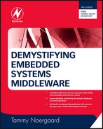
Where a compiler usually translates all of the given source code at one time, an interpreter generates (interprets) machine code one source code line at a time (see Figure 6.4).
One of the most common subclasses of interpreted programming languages is scripting languages, which include PERL, JavaScript, and HTML. Scripting languages are high-level programming languages with enhanced features, including:
• More platform independence than their compiled high-level language counterparts2
• Late binding, which is the resolution of data types on-the-fly (rather than at compile time) to allow for greater flexibility in their resolution2
• Importation and generation of source code at runtime, which is then executed immediately2
• Optimizations for efficient programming and rapid prototyping of certain types of applications, such as internet applications and graphical user interfaces (GUIs).2
With embedded platforms that support programs written in a scripting language, an additional component – an interpreter – must be included in the embedded system’s architecture to allow for ‘on-the-fly’ processing of code. Note that while all scripting languages are interpreted, not all interpreted languages are scripting languages. For example, one popular embedded programming language that incorporates both compiling and interpreting machine code generation methods is Java. On the programmer’s host machine, Java must go through a compilation procedure that generates Java byte code from Java source code (see Figure 6.5).

Java byte code is target code intended to be platform independent. In order for the Java byte code to run on an embedded system, one of the most commonly known types of virtual machines in embedded devices and used as the real-world example in this chapter, called a Java Virtual Machine (JVM), must reside on that system.
Real-world JVMs are currently implemented in an embedded system in one of three ways: in the hardware, as middleware in the system software layer, or in the application layer (see Figure 6.6). Within the scope of this chapter, it is when a virtual machine, like a JVM, is implemented as middleware that is addressed more specifically.

Scripting languages and Java aren’t the only high-level languages that can automatically introduce an additional component as middleware within an embedded system. A real-world VM framework, called the .NET Compact Framework from Microsoft, allows applications written in almost any high-level programming language (such as C#, Visual Basic and Javascript) to run on any embedded device, independent of hardware or system software design.
Applications that fall under the .NET Compact Framework must go through a compilation and linking procedure that generates a CPU-independent intermediate language file, called MSIL (Microsoft Intermediate Language), from the original source code file (see Figure 6.7). For a high-level language to be compatible with the .NET Compact Framework, it must adhere to Microsoft’s Common Language Specification, a publicly available standard that anyone can use to create a compiler that is .NET compatible.

6.2 Understanding the Elements of a VM’s Architecture1
After understanding the basics of programming languages, the key next steps for the reader in demystifying VM middleware include:
Step 2.Understand the APIs that are provided by a VM in support of its inherent purpose. In other words, know your standards relative to VMs that are specific to embedded devices (as first introduced in Chapter 3).
Step 3.Using the Embedded Systems Model, define and understand all required architecture components that underlie the virtual machine, including:
Step 3.1. Understanding the hardware (Chapter 2). If the reader comprehends the hardware, it is easier to understand why a VM implements functionality in a certain way relative to the hardware, as well as the hardware requirements of a particular VM implementation.
Step 3.2. Define and understand the specific underlying system software components, such as the available device drivers supporting the storage medium(s) and the operating system API (Chapter 2).
Step 4.Define the particular virtual machine or VM-framework architecture model, and then define and understand what type of functionality and data exists at each layer. This step will be addressed in the next few pages.
As mentioned at the start of this chapter, a virtual machine (VM) has many similarities in theory to the functionality provided by an embedded operating system (OS). This means a VM provides functionality that will perform everything from process management to memory management to I/O system management in addition to the translation of the higher-level language supported by the particular VM. Size, speed, and available out-of-the-box functionality are the technical characteristics of a VM that most impact an embedded system design, and essentially are the main differentiators of similar VMs provided by competing vendors. These characteristics are impacted by the internal design of three main subsystems within the VM, the:
As shown in Figure 6.8, for example, the .NET Compact Framework is made up of an execution engine referred to as a common language runtime (CLR) at the time this book was written, a class loader, and platform extension libraries. The CLR is made up of an execution engine that processes the intermediate MSIL code into machine code, and a garbage collector. The platform extension libraries are within the base class library (BCL), which provides additional functionality to applications (such as graphics, networking, and diagnostics). In order to run the intermediate MSIL file on an embedded system, the .NET Compact Framework must exist on that embedded system.

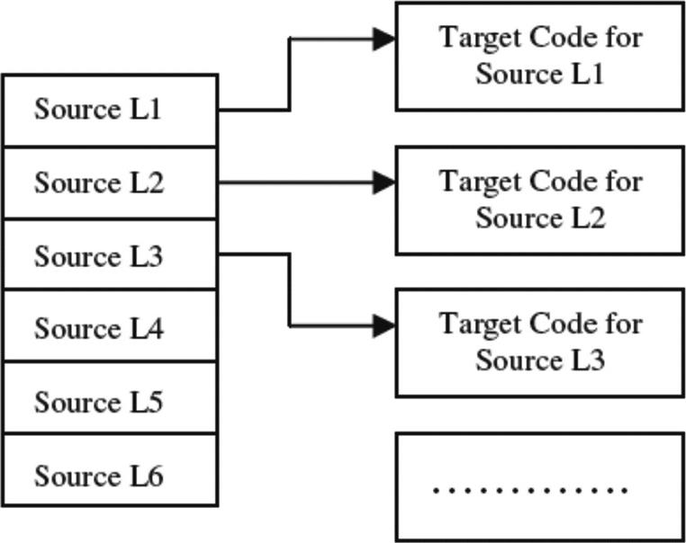
Another example is embedded JVMs implemented as middleware, which are also made up of a loader, execution engine, and Java API libraries (see Figure 6.9). While there are several embedded JVMs available on the market today, the primary differentiators between these JVMs are the JVM classes included with the JVM, and the execution engine that contains components needed to successfully process Java code.
6.2.1 The APIs
The APIs (application program interfaces) are application-independent libraries provided by the VM to, among other things, allow programmers to execute system functions, reuse code, and more quickly create overlying software. Overlying applications that use the VM within the embedded device require the APIs, in addition to their own code, to successfully execute. The size, functionality, and constraints provided by these APIs differ according to the VM specification adhered to, but provided functionality can include memory management features, graphics support, networking support, to name a few. In short, the type of applications in an embedded design is dependent on the APIs provided by the VM.
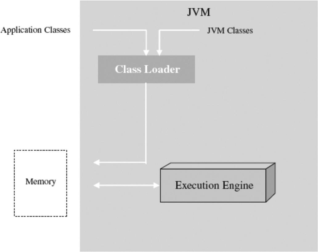
For example, different embedded Java standards with their corresponding APIs are intended for different families of embedded devices (see Figure 6.10). The type of applications in a Java-based design is dependent on the Java APIs provided by the JVM. The functionality provided by these APIs differs according to the Java specification adhered to, such as inclusion of the Real Time Core Specification from the J Consortium, Personal Java (pJava), Embedded Java, Java 2 Micro Edition (J2ME), and The Real Time Specification for Java from Sun Microsystems. Of these embedded Java standards, to date pJava and J2ME standards have typically been the standards implemented within larger embedded devices. PJava 1.1.8 was the predecessor of J2ME CDC that Sun Microsystems targeted to be replaced by J2ME.
Figure 6.11 shows an example of differences between the APIs of two different embedded Java standards.

There are later editions to 1.1.8 of pJava specifications from Sun, but as mentioned J2ME standards were intended to completely phase out the pJava standards in the embedded industry (by Sun) at the time this book was written. However, because the open source example used in this chapter is the Kaffe JVM implementation that is a clean room JVM based upon the pJava specification, this standard will be used as one of the examples to demonstrate functionality that is implemented via a JVM. Using this open source example, though based upon an older embedded Java standard, allows readers to have access to VM source code for hands-on purposes. The key is for the reader to use this open source example to get a clearer understanding of VM implementation from a systems-level perspective, regardless of whether the ‘internal’ functions used to implement one VM versus another differs from another because of the specification that VM adheres to (i.e., pJava versus J2ME, J2ME CDC versus J2ME CLDC, different versions of J2ME CLDC, and so on). The reader can use these examples as tools to understanding any VM implementation encountered, be it home-grown or purchased from a vendor.
To start, a high-level snapshot of the APIs provided by Sun’s pJava standard are shown in Figure 6.12. In the case of a pJava JVM implemented in the system software layer, these libraries would be included (along with the JVM’s loading and execution units) as middleware components.

Using specific networking APIs in the pJava specification as a more detailed example, shown in Figure 6.13 is the java.net package. The JVM provides an upper-transport layer API for remote interprocess communication via the client–server model (where the client requests data, etc., from the server).

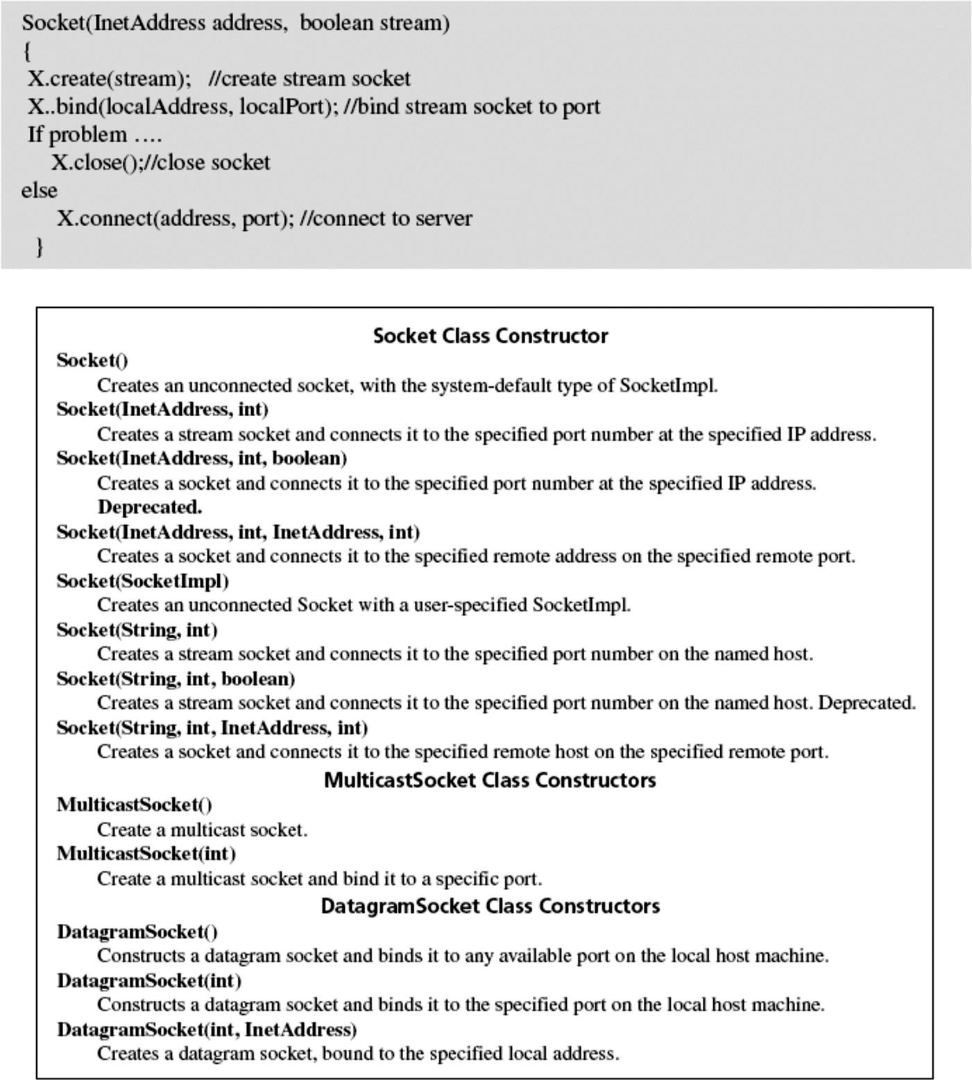
The APIs needed for client and servers are different, but the basis for establishing the network connection via Java is the socket (one at the client end and one at the server end). As shown in Figure 6.14, Java sockets use transport layer protocols of middleware networking components, such as TCP/IP discussed in the previous middleware example. Of the several different types of sockets (raw, sequenced, stream, datagram, etc.), the pJava JVM provides datagram sockets, in which data messages are read in their entirety at one time, and stream sockets, where data are processed as a continuous stream of characters. JVM datagram sockets rely on the UDP transport layer protocol, while stream sockets use the TCP transport layer protocol. pJava provides support for the client and server sockets, specifically one class for datagram sockets (called DatagramSocket, used for either client or server), and two classes for client stream sockets (Socket and MulticastSocket).

A socket is created within a higher-layer application via one of the socket constructor calls, in the DatagramSocket class for a datagram socket, in the Socket class for a stream socket, or in the MulticastSocket class for a stream socket that will be multicast over a network (see Figure 6.15). As shown in the pseudocode example below of a Socket class constructor, within the pJava API, a stream socket is created, bound to a local port on the client device, and then connected to the address of the server.
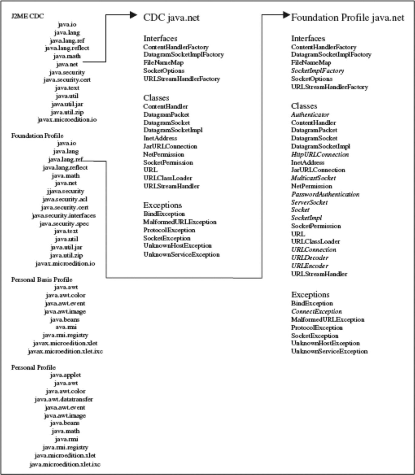
In the J2ME set of standards, there are networking APIs provided by the packages within the CDC configuration and Foundation profile, as shown in Figure 6.18. In contrast to the pJava APIs shown in Figure 6.12, J2ME CDC APIs are a different set of libraries that would be included, along with the JVM’s loading and execution units, as middleware components.
As shown in Figure 6.16, the CDC provides support for the client sockets. Specifically, there is one class for datagram sockets (called DatagramSocket and used for either client or server) under CDC. The Foundation Profile, that sits on top of CDC, provides three classes for stream sockets, two for client sockets (Socket and MulticastSocket) and one for server sockets (ServerSocket). A socket is created within a higher-layer application via one of the socket constructor calls, in the DatagramSocket class for a client or server datagram socket, in the Socket class for a client stream socket, in the MulticastSocket class for a client stream socket that will be multicast over a network, or in the ServerSocket class for a server stream socket, for instance (see Figure 6.16). In short, along with the addition of a server (stream) socket API in J2ME, a device’s middleware layer changes between pJava and J2ME CDC implementations in that the same sockets available in pJava are available in J2ME’s network implementation, just in two different substandards under J2ME as shown in Figure 6.17.

The J2ME connected limited device configuration (CLDC, shown in Figure 6.18) and related profile standards are geared for smaller embedded systems by the Java community.
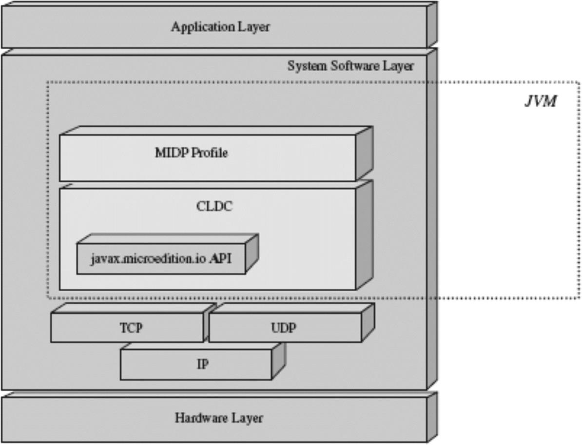
Continuing with networking as an example, the CLDC-based Java APIs provided by a CLDC-based JVM do not provide a .net package, as do the larger JVM implementations (see Figure 6.19).

Under the CLDC implementation, a generic connection is provided that abstracts networking, and the actual implementation is left up to the device designers. The Generic Connection Framework (javax.microedition.io package) consists of one class and seven connection interfaces:
• Connection – closes the connection
• ContentConnection – provides metadata info
• DatagramConnection – create, send, and receive
• InputConnection – opens input connections
• OutputConnection – opens output connections
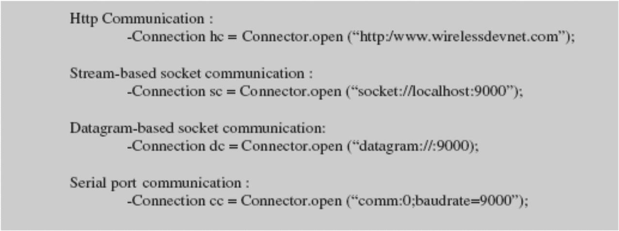
The Connection class contains one method (Connector.open) that supports the file, socket, comm, datagram and http protocols, as shown in Figure 6.20.
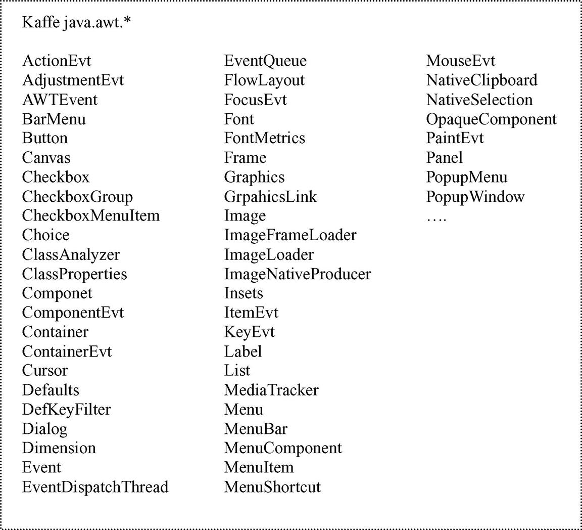
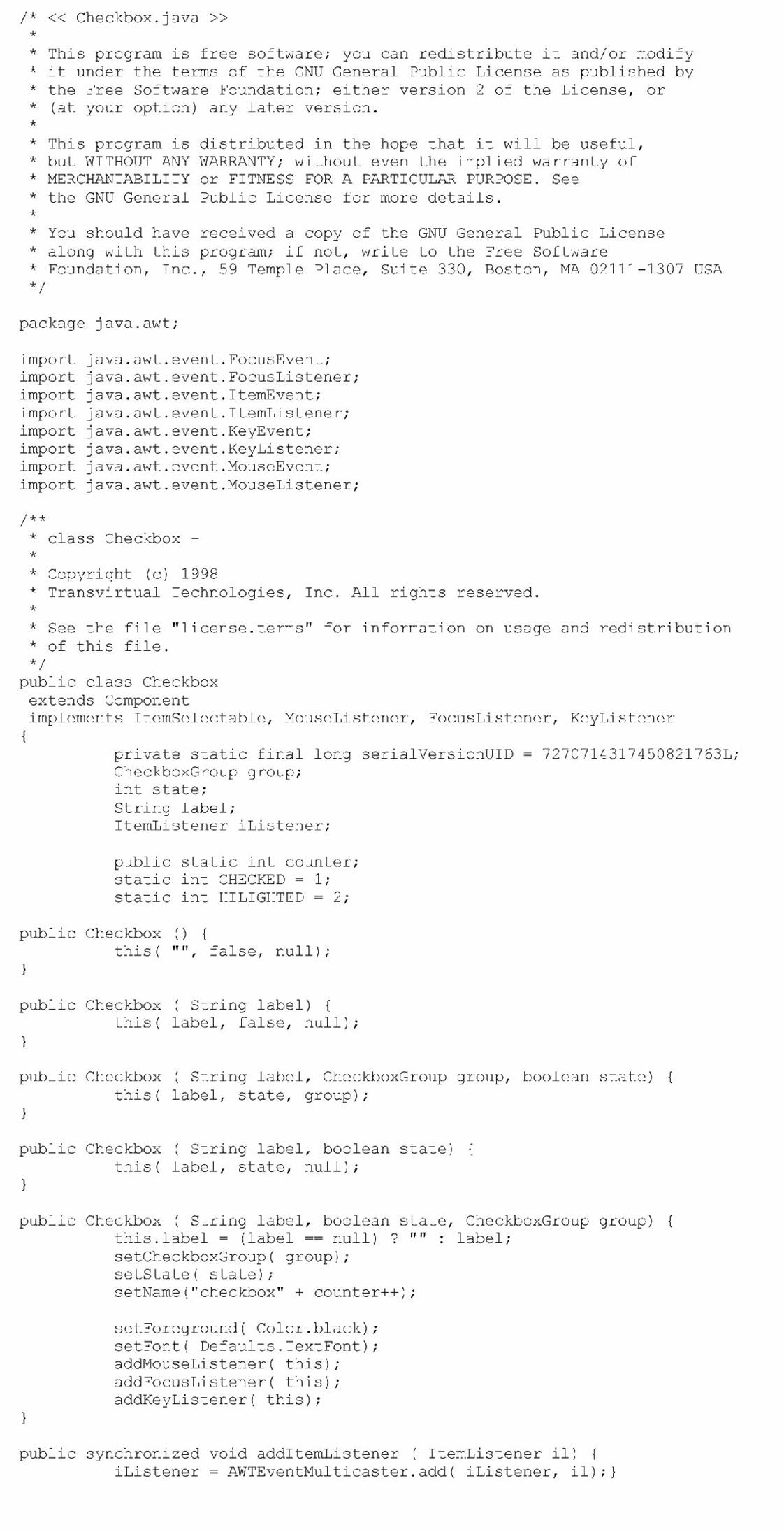
Another example is located within the Kaffe JVM open source example used in this chapter that contains its own implementation of a java.awt graphical library. AWT (abstract window toolkit) is a class library that allows for creating graphical user interfaces in Java. Figures 6.21a, b and c show a list of some of the java.awt libraries, as well as real-world source of one of the awt libraries being implemented.


6.2.2 Execution Engine
Within an execution engine, there are several components that support process, memory, and I/O system management – however, the main differentiators that impact the design and performance of VMs that support the same specification are:
• The units within the VM that are responsible for process management and for translating what is generated on the host into machine code via:
• just-in-time (JIT), an algorithm that combines both compiling and interpreting
• ahead-of-time compilation, such as dynamic adaptive compilers (DAC), ahead-of-time, way-ahead-of-time (WAT) algorithms to name a few.
A VM can implement one or more of these processing algorithms within its execution engine.
• The memory management scheme that includes a garbage collector (GC), which is responsible for deallocating any memory no longer needed by the overlying application.
With interpretation in a JVM, shown in Figure 6.22 for example, every time the Java program is loaded to be executed, every byte code instruction is parsed and converted to native code, one byte code at a time, by the JVM’s interpreter. Moreover, with interpretation, redundant portions of the code are reinterpreted every time they are run. Interpretation tends to have the lowest performance of the three algorithms, but it is typically the simplest algorithm to implement and to port to different types of hardware.

A JIT compiler (see Figure 6.23), on the other hand, interprets the program once, and then compiles and stores the native form of the byte code at runtime, thus allowing redundant code to be executed without having to reinterpret. The JIT algorithm performs better for redundant code, but it can have additional runtime overhead while converting the byte code into native code. Additional memory is also used for storing both the Java byte codes and the native compiled code. Variations on the JIT algorithm in real-world JVMs are also referred to as translators or dynamic adaptive compilation (DAC).

Finally, as shown in Figure 6.24, in WAT/AOT compiling all Java byte code is compiled into the native code at compile time, as with native languages, and no interpretation is done. This algorithm performs at least as well as the JIT for redundant code and better than a JIT for non-redundant code, but as with the JIT, there is additional runtime overhead when additional Java classes dynamically downloaded at runtime have to be compiled and introduced to the system. WAT/AOT can also be a more complex algorithm to implement.

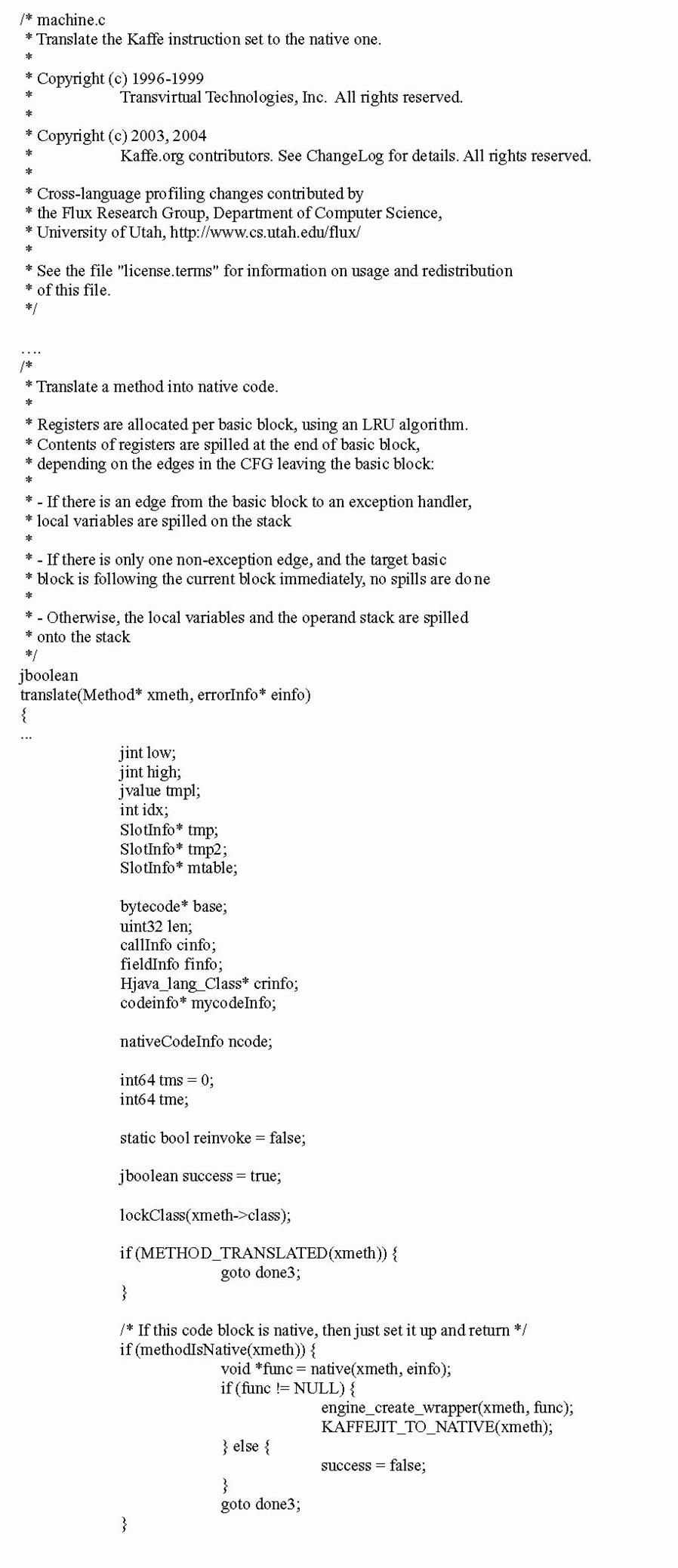
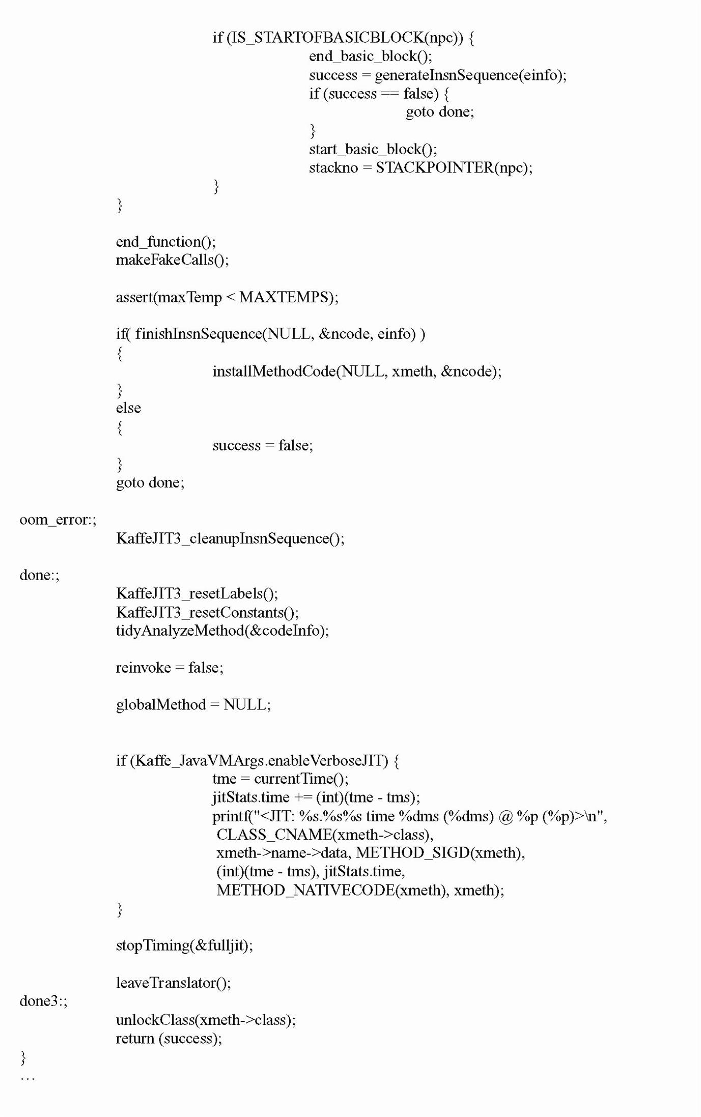
The Kaffe open source example used in this chapter contains a JIT (just-in-time) compiler called JIT3 (JIT version 3). The translate function shown in Figure 6.25 is the root of Kaffe’s JIT3.3 In general, the Kaffe JIT compiler performs three main functions:7
1. Byte code analysis. A codeinfo structure is generated by the ‘verifyMethod’ function that contains relevant data including:
2. Instruction translation and machine code generation. Byte code translation is done at an individual block level generally as follows:
a. Pass 1. Byte codes are mapped into intermediate functions and macros. A list of sequence objects containing master architecture-specific data are then generated.
b. Pass 2. The sequence objects are used to generate the architecture-specific native instruction code.
3. Linking. The generated code is linked into the VM after all blocks have been processed. The native instruction code is then copied and linked.


6.2.2.1 Tasks versus Threads in Embedded VMs
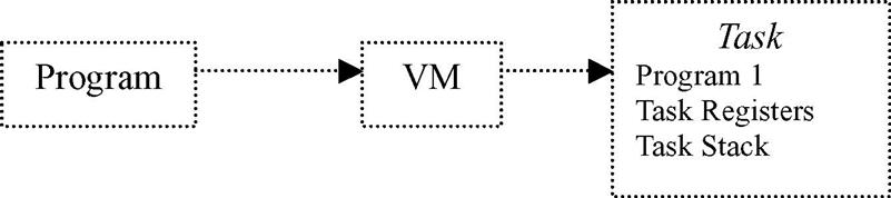
As with operating systems, VMs manage and view other (overlying) software within the embedded system via some process management scheme. The complexity of a VM process management scheme will vary from VM to VM; however, in general the process management scheme is how a VM differentiates between an overlying program and the execution of that program. To a VM, a program is simply a passive, static sequence of instructions that could represent a system’s hardware and software resources. The actual execution of a program is an active, dynamic event in which various properties change relative to time and the instruction being executed. A process (also commonly referred to as a task) is created to encapsulate all the information that is involved in the executing of a program (i.e., stack, PC, the source code and data, etc.). This means that a program is only part of a task, as shown in Figure 6.26a.
Many embedded VMs also provide threads (lightweight processes) as an alternative means for encapsulating an instance of a program. Threads are created within the context of the OS task in which the VM is running, meaning all VM threads are bound to the VM task, and is a sequential execution stream within the task.
Unlike tasks, which have their own independent memory spaces that are inaccessible to other tasks, threads of a task share the same resources (working directories, files, I/O devices, global data, address space, program code, etc.), but have their own PCs, stack, and scheduling information (PC, SP, stack, registers, etc.) to allow for the instructions they are executing to be scheduled independently. Since threads are created within the context of the same task and can share the same memory space, they can allow for simpler communication and coordination relative to tasks. This is because a task can contain at least one thread executing one program in one address space, or can contain many threads executing different portions of one program in one address space (see Figure 6.26b), needing no intertask communication mechanisms. Also, in the case of shared resources, multiple threads are typically less expensive than creating multiple tasks to do the same work.

VMs must manage and synchronize tasks (or threads) that can exist simultaneously because, even when a VM allows multiple tasks (or threads) to coexist, one master processor on an embedded board can only execute one task or thread at any given time. As a result, multitasking embedded VMs must find some way of allocating each task a certain amount of time to use the master CPU, and switching the master processor between the various tasks. This is accomplished through task implementation, scheduling, synchronization, and inter-task communication mechanisms.
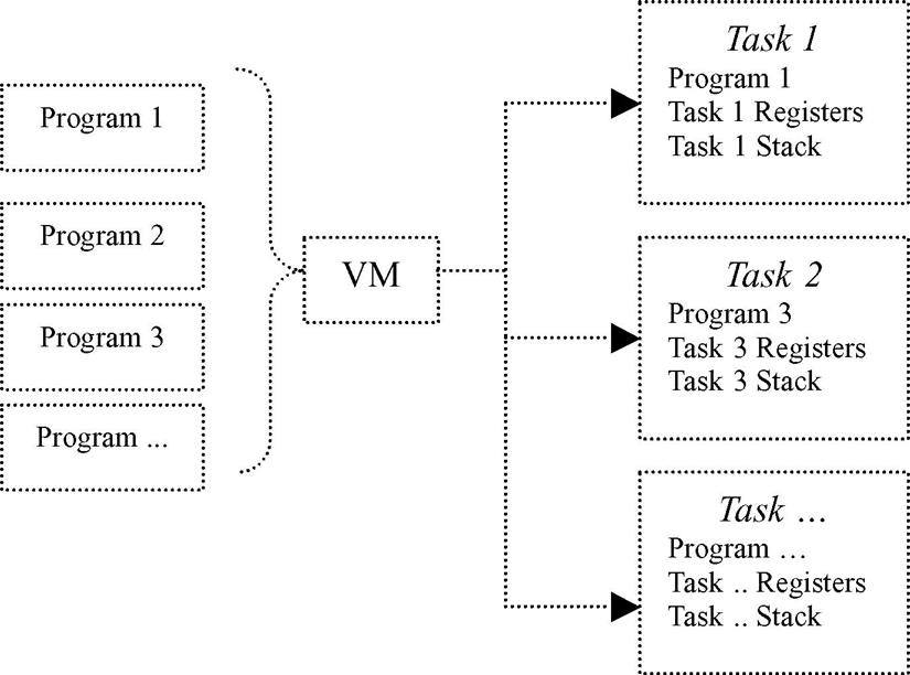
Jbed is a real-world example of a JVM that provides a task-based process management scheme that supports a multitasking environment. What this means is that multiple Java-based tasks are allowed to exist simultaneously, where each Jbed task remains independent of the others and does not affect any other Java task without the specific programming to do so (see Figure 6.27).
Jbed, for example, provides six different types of tasks that run alongside threads: OneshotTimer Task (which is a task that is run only once), PeriodicTimer Task (a task that is run after a particular set time interval), HarmonicEvent Task (a task that runs alongside a periodic timer task), JoinEvent Task (a task that is set to run when an associated task completes), InterruptEvent Task (a task that is run when a hardware interrupt occurs), and the UserEvent Task (a task that is explicitly triggered by another task). Task creation in Jbed is based upon a variation of the spawn model, called spawn threading. Spawn threading is spawning, but typically with less overhead and with tasks sharing the same memory space.
Figure 6.28 is a pseudocode example of task creation of a OneShot task, one of Jbed’s six different types of tasks, in the Jbed RTOS where a parent task ‘spawns’ a child task software timer that runs only one time. The creation and initialization of the Task object is the Jbed (Java) equivalent of a task control block (TCB) which contains for that particular task data such as task ID, task state, task priority, error status, and CPU context information to name a few examples. The task object, along with all objects in Jbed, is located in Jbed’s heap (in a JVM, there is typically only one heap for all objects). Each task in Jbed is also allocated its own stack to store primitive data types and object references.

Because Jbed is based upon the JVM model, a garbage collector (introduced in the next section of this chapter) is responsible for deleting a task and removing any unused code from memory once the task has stopped running. Jbed uses a non-blocking mark-and-sweep garbage collection algorithm which marks all objects still being used by the system and deletes (sweeps) all unmarked objects in memory.
In addition to creating and deleting tasks, a VM will typically provide the ability to suspend a task (meaning temporarily blocking a task from executing) and resume a task (meaning any blocking of the task’s ability to execute is removed). These two additional functions are provided by the VM to support task states. A task’s state is the activity (if any) that is going on with that task once it has been created, but has not been deleted.
Tasks are usually defined as being in one of three states:
• Ready: The process is ready to be executed at any time, but is waiting for permission to use the CPU.
• Running: The process has been given permission to use the CPU, and can execute.
• Blocked or Waiting: The process is waiting for some external event to occur before it can be ‘ready’ to ‘run’.
Based upon these three states (Ready, Blocked, and Running), Jbed (for example) as a process state transition model is shown in Figure 6.29. In Jbed, some states of tasks are related to the type of task, as shown in the table and state diagrams below. Jbed also uses separate queues to hold the task objects that are in the various states.

The Kaffe open source JVM implements priority-preemptive-based ‘jthreads’ on top of OS native threads. Figure 6.30 shows a snapshot of Kaffe’s thread creation and deletion scheme.


6.2.2.2 Embedded VMs and Scheduling
VM mechanisms, such as a scheduler within an embedded VM, are one of the main elements that give the illusion of a single processor simultaneously running multiple tasks or threads (see Figure 6.31). A scheduler is responsible for determining the order and the duration of tasks (or threads) to run on the CPU. The scheduler selects which tasks will be in what states (Ready, Running, or Blocked), as well as loading and saving the information for each task or thread.

There are many scheduling algorithms implemented in embedded VMs, and every design has its strengths and tradeoffs. The key factors that impact the effectiveness and performance of a scheduling algorithm include its response time (time for scheduler to make the context switch to a ready task and includes waiting time of task in ready queue), turnaround time (the time it takes for a process to complete running), overhead (the time and data needed to determine which tasks will run next), and fairness (what are the determining factors as to which processes get to run). A scheduler needs to balance utilizing the system’s resources – keeping the CPU, I/O, as busy as possible – with task throughput, processing as many tasks as possible in a given amount of time. Especially in the case of fairness, the scheduler has to ensure that task starvation, where a task never gets to run, doesn’t occur when trying to achieve a maximum task throughput.
One of the biggest differentiators between the scheduling algorithms implemented within embedded VMs is whether the algorithm guarantees its tasks will meet execution time deadlines. Thus, it is important to determine whether the embedded VM implements a scheduling algorithm that is non-preemptive or preemptive. In preemptive scheduling, the VM forces a context-switch on a task, whether or not a running task has completed executing or is cooperating with the context switch. Under non-preemptive scheduling, tasks (or threads) are given control of the master CPU until they have finished execution, regardless of the length of time or the importance of the other tasks that are waiting. Non-preemptive algorithms can be riskier to support since an assumption must be made that no one task will execute in an infinite loop, shutting out all other tasks from the master CPU. However, VMs that support non-preemptive algorithms don’t force a context-switch before a task is ready, and the overhead of saving and restoration of accurate task information when switching between tasks that have not finished execution is only an issue if the non-preemptive scheduler implements a cooperative scheduling mechanism.
As shown in Figure 6.32, Jbed contains an earliest deadline first (EDF)-based scheduler where the EDF/Clock Driven algorithm schedules priorities to processes according to three parameters: frequency (number of times process is run), deadline (when processes execution needs to be completed), and duration (time it takes to execute the process). While the EDF algorithm allows for timing constraints to be verified and enforced (basically guaranteed deadlines for all tasks), the difficulty is defining an exact duration for various processes. Usually, an average estimate is the best that can be done for each process.

Under the Jbed RTOS, all six types of tasks have the three variables ‘duration’, ‘allowance’, and ‘deadline’ when the task is created for the EDF scheduler to schedule all tasks (see Figure 6.33 for the method call).

The Kaffe open source JVM implements a priority-preemptive-based scheme on top of OS native threads, meaning jthreads are scheduled based upon their relative importance to each other and the system. Every jthread is assigned a priority, which acts as an indicator of orders of precedence within the system. The jthreads with the highest priority always preempt lower-priority processes when they want to run, meaning a running task can be forced to block by the scheduler if a higher-priority jthread becomes ready to run. Figure 6.34 shows three jthreads (1, 2, 3 – where jthread 1 is the lowest priority and jthread 3 is the highest, and jthread 3 preempts jthread 2, and jthread 2 preempts jthread 1).

As with any VM with a priority-preemptive scheduling scheme, the challenges that need to be addressed by programmers include:
• JThread starvation, where a continuous stream of high-priority threads keeps lower-priority jthreads from ever running. Typically resolved by aging lower-priority jthreads (as these jthreads spend more time on queue, increase their priority levels).
• Priority inversion, where higher-priority jthreads may be blocked waiting for lower-priority jthreads to execute, and jthreads with priorities in between have a higher priority in running, thus both the lower-priority as well as higher-priority jthreads don’t run (see Figure 6.35).
• How to determine the priorities of various threads. Typically, the more important the thread, the higher the priority it should be assigned. For jthreads that are equally important, one technique that can be used to assign jthread priorities is the Rate Monotonic Scheduling (RMS) scheme which is also commonly used with relative scheduling scenerios when using embedded OSs. Under RMS, jthreads are assigned a priority based upon how often they execute within the system. The premise behind this model is that, given a preemptive scheduler and a set of jthreads that are completely independent (no shared data or resources) and are run periodically (meaning run at regular time intervals), the more often a jthread is executed within this set, the higher its priority should be. The RMS Theorem says that if the above assumptions are met for a scheduler and a set of ‘n’ jthreads, all timing deadlines will be met if the inequality Σ Ei/Ti ≤ n(21/n – 1) is verified, where
n = number of periodic jthreads
Ti = the execution period of jthread i
Ei = the worst-case execution time of jthread i
Ei/Ti = the fraction of CPU time required to execute jthread i.

So, given two jthreads that have been prioritized according to their periods, where the shortest-period jthread has been assigned the highest priority, the ‘n(21/n – 1)’ portion of the inequality would equal approximately 0.828, meaning the CPU utilization of these jthreads should not exceed about 82.8% in order to meet all hard deadlines. For 100 jthreads that have been prioritized according to their periods, where the shorter period jthreads have been assigned the higher priorities, CPU utilization of these tasks should not exceed approximately 69.6% (100 × (21/100 − 1)) in order to meet all deadlines. See Figure 6.36 for additional notes on this type of scheduling model.

6.2.2.3 VM Memory Management and the Garbage Collector1
A VM’s memory heap space is shared by all the different overlying VM processes – so access, allocation, and deallocation of portions of the heap space need to be managed. In the case of VMs, a garbage collector (GC) is integrated within. Garbage collection discussed in this chapter isn’t necessarily unique to any particular language. A garbage collector (GC) can be implemented within embedded devices in support of other languages that do not require VMs, such as C and C++.8 Regardless, when creating a garbage collector to support any language, it becomes an integral component of an embedded system’s architecture.
Applications written in a language such as Java or C# all utilize the same memory heap space of the VM and cannot allocate or deallocate memory in this heap or outside this heap that has been allocated for previous use (as can be done in native languages, such as using ‘free’ in the C language, though as mentioned above, a garbage collector can be implemented to support any language). In Java, for example, only the GC (garbage collector) can deallocate memory no longer in use by Java applications. GCs are provided as a safety mechanism for Java programmers so they do not accidentally deallocate objects that are still in use. While there are several garbage collection schemes, the most common are based upon the copying, mark and sweep, and generational GC algorithms.
6.2.2.4 GC Memory Allocator1
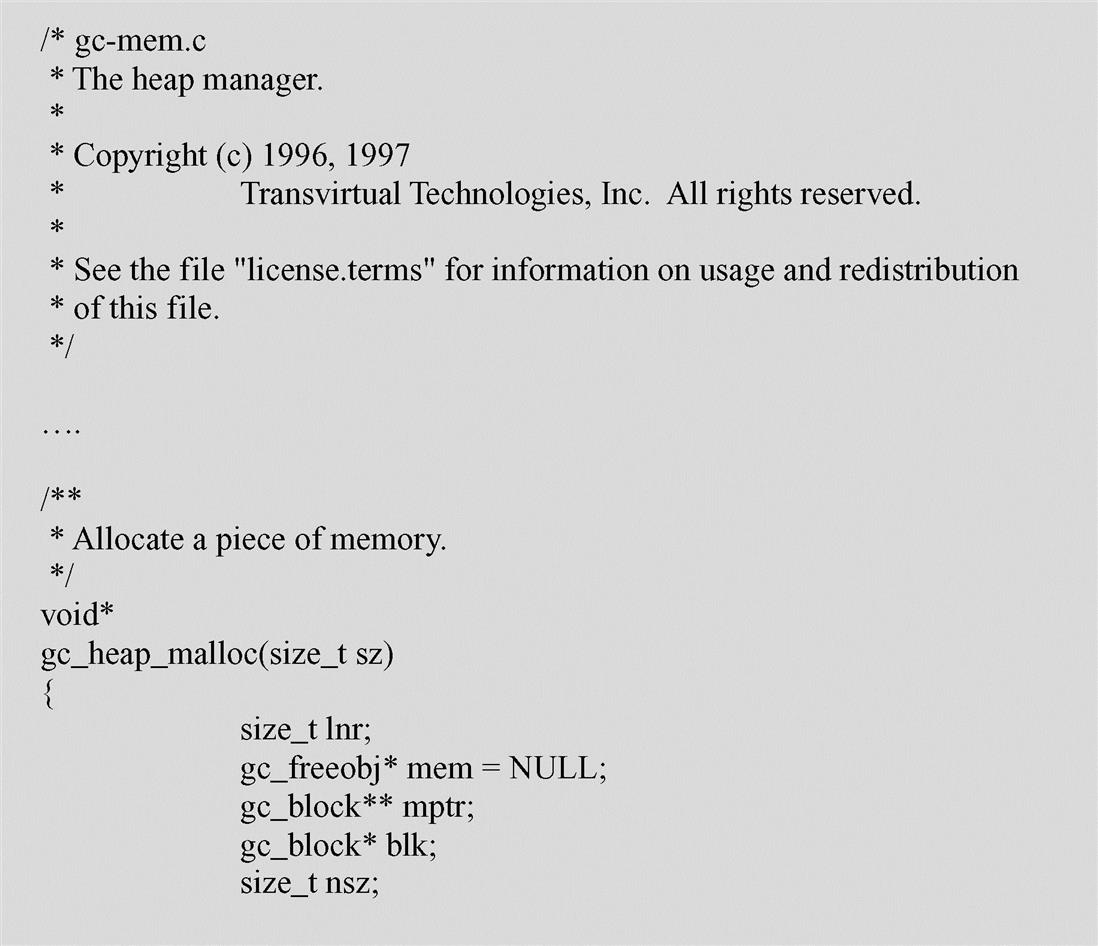
Embedded VMs can implement a wide variety of schemes to manage the allocation of the memory heap, in combination with an underlying operating system’s memory management scheme. With Kaffe, for example, the GC including a memory allocator for the JVM in addition to the underlying operating system’s memory management scheme is utilized. When Kaffe’s memory allocator is used to allocate memory (see Figure 6.37) from the JVMs heap space, its purpose is to simply determine if there is free memory to allocate – and if so, returning this memory for use.

6.2.2.5 Garbage Collection1
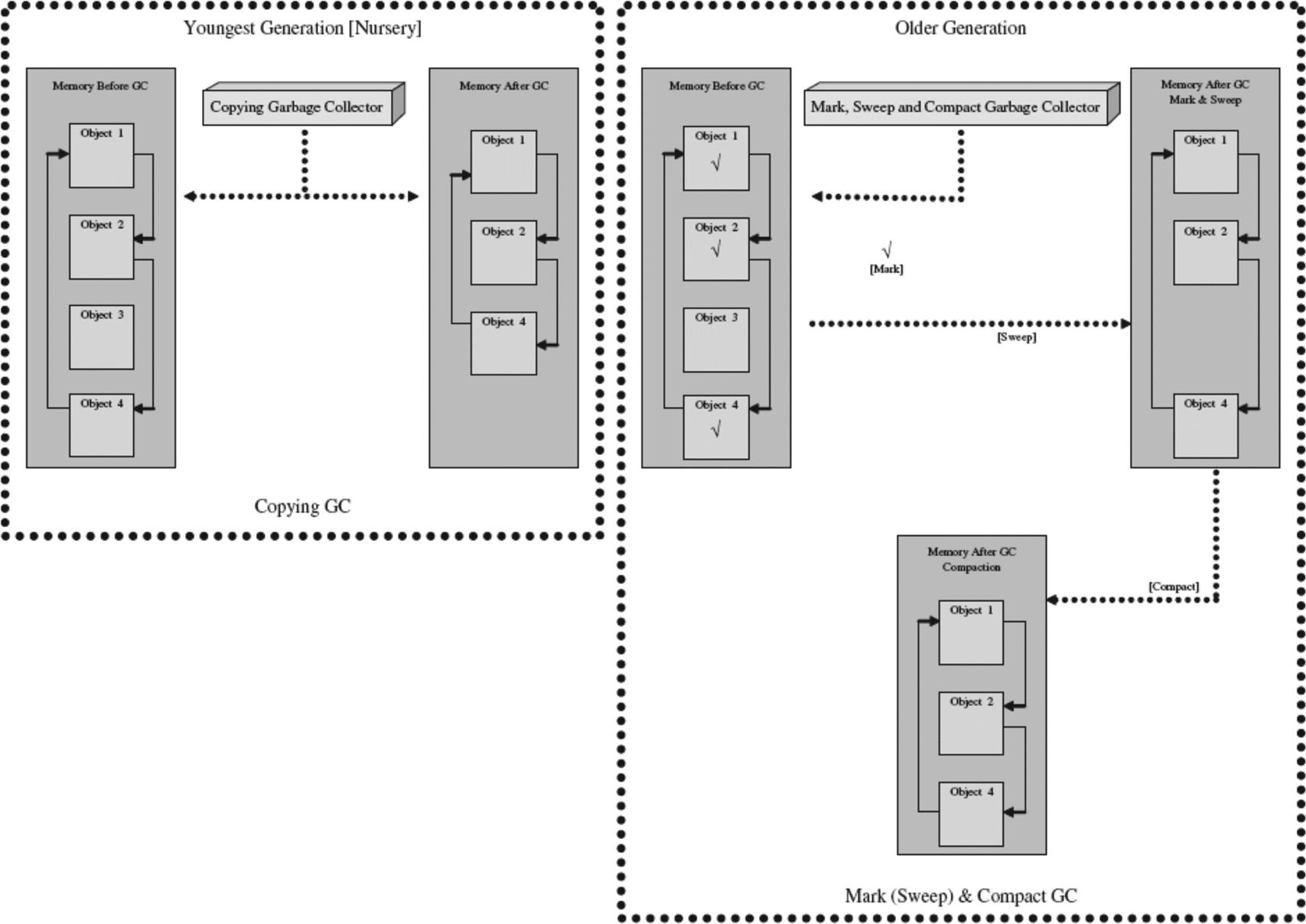
The copying garbage collection algorithm (shown in Figure 6.38) works by copying referenced objects to a different part of memory, and then freeing up the original memory space of unreferenced objects. This algorithm uses a larger memory area in order to work, and usually cannot be interrupted during the copy (it blocks the system). However, it does ensure that what memory is used is used efficiently by compacting objects in the new memory space.

The mark and sweep garbage collection algorithm (shown in Figure 6.39) works by ‘marking’ all objects that are used, and then ‘sweeping’ (deallocating) objects that are unmarked. This algorithm is usually non-blocking, meaning the system can interrupt the garbage collector to execute other functions when necessary. However, it doesn’t compact memory the way a copying garbage collector does, leading to memory fragmentation, the existence of small, unusable holes where deallocated objects used to exist. With a mark and sweep garbage collector, an additional memory compacting algorithm can be implemented, making it a mark (sweep) and compact algorithm.

Finally, the generational garbage collection algorithm (shown in Figure 6.40) separates objects into groups, called generations, according to when they were allocated in memory. This algorithm assumes that most objects that are allocated by a Java program are short-lived, thus copying or compacting the remaining objects with longer lifetimes is a waste of time. So, it is objects in the younger-generation group that are cleaned up more frequently than objects in the older-generation groups. Objects can also be moved from a younger-generation to an older-generation group. Different generational garbage collectors also may employ different algorithms to deallocate objects within each generational group, such as the copying algorithm or mark and sweep algorithms described previously.
The Kaffe open source example used in this chapter implements a version of a mark and sweep garbage collection algorithm. In short, the garbage collector (GC) within Kaffe will be invoked when the memory allocator determined more memory is required than free memory in the heap. The GC then schedules when the garbage collection will occur, and executes the collection (freeing of memory) accordingly. Figure 6.41 shows Kaffe’s open source example of a mark and sweep GC algorithm for ‘marking’ data for collection.

6.2.3 VM Memory Management and the Loader
The loader is simply as its name implies. As shown in Figure 6.42a, it is responsible for acquiring and loading into memory all required code in order to execute the relative program overlying the VM. In the case of a JVM like Kaffe, for example (see Figure 6.42b for open source snapshot), its internal Java class loader loads into memory all required Java classes required for the Java program to function.


6.3 A Quick Comment on Selecting Embedded VMs Relative to the Application Layer
Writing applications in a higher-level language that requires introducing an underlying VM in the middleware layer of an embedded system design, for better or worse, will require additional support relative to increased processing power and memory requirements. This is opposed to implementing the same applications in native C and/or assembly. So, as with integrating any type of middleware component, introducing a VM into an embedded system means planning for any additional hardware requirements and underlying system software by both the VM and the overlying applications that utilize the underlying VM middleware component. This is where understanding the fundamentals of the internal design of VMs, like the material presented in previous sections of this chapter, becomes critical to selecting the best design that meets your particular device’s requirements.
For example, several factors, such as memory and performance, are impacted by the scheme a VM utilizes in processing the overlying application code. So, understanding the pros and cons of using a particular JVM that implements an interpretating byte-code scheme versus a just-in-time (JIT) compiler versus a way-ahead-of-time (WAT) compiler versus a dynamic adaptive compiler (DAC) is necessary. This means that, while using a particular JVM with a certain compilation scheme would introduce significant performance improvements, it may also introduce requirements for additional memory as well as introduce other limitations. For instance, pay close attention to the drawbacks to selecting a particular JVM that utilizes some type of ahead-of-time (AOT) or way-ahead-of-time (WAT) compilation which provides a big boost in performance when running on your hardware, but lacks the ability to process dynamically downloaded Java byte-code, whereas this dynamic download capability is provided by a competing JVM solution based on a slower, interpretating byte-code processing scheme. If on-the-field dynamic extensibility support is a non-negotiable requirement for the embedded system being designed, then it means needing to investigate further other options such as:
• selecting a competing JVM from another vendor that provides this dynamic-download capability out-of-the-box
• investigating the feasibility of deploying with a JVM based on a different byte-code processing scheme that runs a bit slower than the faster JVM solution that lacks dynamic download and extensibility support
• planning the resources, costs, and time to implement this required functionality within the scope of the project.
Another example would be when having to decide between a JIT implementation of a JVM versus going with the JIT-based .NET Compact Framework solution of comparable performance on your particular hardware and underlying system software. In addition to examining the available APIs provided by the JVM versus .NET Compact Framework embedded solutions for your application requirements, do not forget to consider the non-technical aspects of going with either particular solution as well. For example, this means taking into consideration when selecting between such alternative VM solutions, the availability of experienced programmers (i.e., Java versus C# programmers for instance). If there are no programmers available with the necessary skills for application development on that particular VM, factor in the costs and time involved in finding and hiring new resources, training current resources, and so on.
Finally do not forget that integrating the right VM in the right manner within the software stack which optimizes the performance of the solution is not enough to insure the design makes it to production successfully. To insure success taking an embedded design that introduces the complexity and stress to underlying components that incorporating an embedded VM produces, requires programmers to plan carefully how overlying applications will be written. This means it is not the most elegant nor the most brilliantly written application code that will insure the success of the design – but simply programmers that design applications in a manner that properly utilizes the underlying VM’s powerful strengths and avoids its weaknesses. A Java application, for example, that is written as a masterpiece by even the cleverest programming guru will not be worth much, if when it runs on the device it was intended for this application is so slow and/or consumes so much of the embedded system’s resources that the device simply cannot be shipped!
In short, the key to selecting which embedded VMs best match the requirements of your design, and successfully taking this design to production within schedule and costs, includes:
• determining if the VM has been ported to your target hardware’s master CPU’s architecture in the first place. If not, it means determining how much time, cost, and resources would be required to port the particular VM to your target hardware and underlying system software stack
• calculating additional processing power and memory requirements to support the VM solution and overlying applications
• specifying what additional type of support and/or porting is needed by the VM relative to underlying embedded OS and/or other middleware system software
• investigating the stability and reliability of the VM implementation on real hardware and underlying system software
• planning around the availability of experienced developers
• evaluating development and debugging tool support
• checking up on the reputation of vendors
• insuring access to solid technical support for the VM implementation for developers
6.4 Summary
This chapter introduced embedded VMs, and their function within an embedded device. A section on programming languages and the higher-level languages that introduce the requirement of a VM within an embedded system was included in this chapter. The major components that make up most embedded VMs were discussed, such as an execution engine, the garbage collector, and loader to name a few. More detailed discussions of process management, memory management, and I/O system management relative to VMs and their architectural components were also addressed in this chapter. Embedded Java virtual machines (JVMs) and the .NET Compact Framework were utilized as real-world examples to demonstrate concepts.
The next chapter in this section introduces database concepts, as related to embedded systems middleware.
6.5 Problems
1. What is a VM? What are the main components that make up a VM’s architecture?
A. In order to run Java, what is required on the target?
B. How can the JVM be implemented in an embedded system?
3. Which standards below are embedded Java standards?
B. RTSC – Real Time Core Specification
C. HTML – Hypertext Markup Language
4. What are the main differences between all embedded JVMs?
5. Name and describe three of the most common byte processing schemes.
A. What is the purpose of a GC?
B. Name and describe two common GC schemes.
A. Name three qualities that Java and scripting languages have in common.
B. Name two ways that they differ.
A. What is the .NET Compact Framework?
9. The .NET compact framework is implemented in the device driver layer of the Embedded Systems Model (True/False).
A. Name three embedded JVM standards that can be implemented in middleware.
B. What are the differences between the APIs of these standards?
C. List two real-world JVMs that support each of the standards.
11. VMs do not support process management (True/False).
12. Define and describe two types of scheduling schemes in VMs.
13. How does a VM typically perform memory management? Name and describe at least two components that VMs can contain to perform memory management.