4
Efficient Computations for (min,plus) Operators
As briefly presented in the Introduction, network calculus is based on computing (min,plus) operators on functions. For some classes of functions, the operations are simple to perform and explicit expressions are given in section 3.1. This is the case for token-bucket, rate-latency and pure delay functions, which are widely used in the network calculus framework. In some other cases, the functions are too complex and efficient algorithms need to be designed to perform the operations.
The aim of this chapter is to provide efficient algorithms to perform the (min,plus) operations. Algorithms can be given for very general functions. However, when functions have a simple enough shape, it is more efficient to use specific algorithms.
We will have a special focus on the class of convex or concave functions. We have already seen in section 3.3 that those functions have good properties with regard to the (min,plus) operators, and we can benefit from them. For example, a token-bucket function is concave and used to model a flow (or arrival process). In some other examples, it is more accurate to model flows by a minimum of two such functions, or by ![]() . This is the case for Traffic Specification (TSpec) [SHE 97] of the Internet Engineering Task Force (IETF): a flow is characterized by a peak rate p, an average or token rate r and a bucket depth b. The function modeling the flow is concave and represented in Figure 4.1. Similarly, the functions modeling a server will often be convex.
. This is the case for Traffic Specification (TSpec) [SHE 97] of the Internet Engineering Task Force (IETF): a flow is characterized by a peak rate p, an average or token rate r and a bucket depth b. The function modeling the flow is concave and represented in Figure 4.1. Similarly, the functions modeling a server will often be convex.
This chapter is organized as follows: in section 4.1, we define the classes of functions that we will study. In section 4.2, we mainly focus on the (min,plus) convolutions of concave and convex functions, as very efficient algorithms exist for these classes of functions.

Figure 4.1. IETF TSpec flow specification. For a color version of this figure, see www.iste.co.uk/bouillard/calculus.zip
Section 4.3 is devoted to the generic algorithms, which can be applied to any function, provided that the result can be finitely represented. For this reason, we restrict ourselves to a class of functions that is stable for all the operators.
Given a flow, several functions can represent it. The more accurate the representation is, the more complex the function must be. Hence, generic algorithms are useful. Sometimes coping with convex and concave functions is a good trade-off. Section 4.4 is devoted to the quantification of this trade-off: functions are approximated by containers, and safe approximations can be computed in quasi-linear time.
Several other approaches have been developed to mitigate the computation cost while still having satisfactory accuracy. One solution is to have an accurate representation of an initial part of the functions, and to only use a linear approximation for the tail of the function, [GUA 13, SUP 10, LAM 16]. Such approximations (see Proposition 5.13) are often sufficient. Another solution is to maintain two approximations of the same curve and to switch from one to the other, depending on the operation to compute [BOY 11b].
4.1. Classes of functions with finite representations
In this section, we introduce the classes of functions used in this chapter. Indeed, our aim is to have efficient representations of the functions, in order to efficiently compute operations on them. The first constraint is that functions can be finitely represented. A simple solution (that is, not restrictive from the application point of view) is to deal with piecewise linear functions only. This way, a function is represented by a list of segments. The second constraint is the stability of the functions with the operators, and we will need to define other properties on the functions. In this section, we define all of the properties that we will need in the rest of the chapter, particularly for section 4.3.
Here, consider functions with definition domain ![]() that take values in
that take values in ![]() . As we will consider dual operations (maximum and minimum), we do not use properties of the dioid properties for infinite values, and some operations may not be defined (e.g.
. As we will consider dual operations (maximum and minimum), we do not use properties of the dioid properties for infinite values, and some operations may not be defined (e.g. ![]() is not well defined). Those cases are easily detected, and we will not consider them: if they are encountered, the result will be considered as undefined.
is not well defined). Those cases are easily detected, and we will not consider them: if they are encountered, the result will be considered as undefined.
Asymptotic behavior of functions:
- – f is a linear function if there exist b and r such that, for all
 ;
; - – f is an ultimately linear function if there exist
 and r such that, for all
  ;
; - – f is a pseudo-periodic function with period d and increment c if, for all
 ,
,  ;
; - – f is an ultimately pseudo-periodic function with period d and increment c if there exists
 such that
  ;
; - – f is a plain function if either, for all
 or there exists
  and
and  such that, for
  (or
(or  ),
),  and, for all
  (or
(or  ),
),  .
.
For ultimately linear and pseudo-periodic functions, T is called a rank of the function. It can be chosen to be minimal and, in that case, it is called the rank (from which the function is linear or ultimately pseudo-periodic). For pseudo-periodic and ultimately pseudo-periodic functions, d is called a period and c an increment. We call ![]() the growth rate of the function. Remark that an (ultimately) linear function is (ultimately) pseudo-periodic with period 1 and increment r. If there exists a minimal
the growth rate of the function. Remark that an (ultimately) linear function is (ultimately) pseudo-periodic with period 1 and increment r. If there exists a minimal ![]() such that a function is (ultimately) pseudo-periodic, this minimal d is the period of the function. This minimal d does not exist if the function is (ultimately) linear.
such that a function is (ultimately) pseudo-periodic, this minimal d is the period of the function. This minimal d does not exist if the function is (ultimately) linear.
Piecewise linear functions. A segment is a function whose support is an interval and which is linear on its support and ![]() outside. If f is such a function, we write
outside. If f is such a function, we write ![]() , where
, where ![]() is the support of f. We will denote by
is the support of f. We will denote by ![]() the growth rate of f on its support, which is also called the slope of f. Note that we do not set any restriction on the shape of the interval. In particular, it can be open, closed, semi-open, a singleton or a semi-line.
the growth rate of f on its support, which is also called the slope of f. Note that we do not set any restriction on the shape of the interval. In particular, it can be open, closed, semi-open, a singleton or a semi-line.
A piecewise linear function is a function that can be written as the minimum of segments and that is the minimum of a finite number of segments on every finite interval.
The decomposition of a piecewise linear function f is a minimum sequence of segments ![]() with disjoint support. It is minimum in the sense that there is no
with disjoint support. It is minimum in the sense that there is no ![]() , such that
, such that ![]() is a segment.
is a segment.
Let X and Y be two sets, and f be a piecewise linear function with representation ![]() . Let
. Let ![]() and
and ![]() be the respective left and right extremities of
be the respective left and right extremities of ![]() . Then,
. Then, ![]() if for all
if for all ![]() and
and ![]()
![]() . We will particularly focus on
. We will particularly focus on ![]() , where
, where ![]() is the set of rational numbers.
is the set of rational numbers.
4.2. Piecewise linear concave/convex functions
The piecewise linear concave and convex functions are certainly the best trade-off between accuracy of modeling and simplicity of implementation. These functions are illustrated in Figure 4.2.

Figure 4.2. Piecewise linear functions: f is concave and g is convex. For a color version of this figure, see www.iste.co.uk/bouillard/calculus.zip
The class of concave piecewise linear functions has nice mathematical properties: it is stable under the addition and minimum operations. Moreover, the (min,plus) convolution (from Proposition 3.12(4)) can be implemented as a minimum plus a constant).
The class of convex piecewise linear functions has very similar properties, replacing minimum with maximum, and its (min,plus) convolution can also be implemented very efficiently, as will be shown in section 4.2.2.1.
In the next section, we will see that there are two equivalent ways of describing piecewise linear function, and in section 4.2.2, we will discuss the implementation of the (min,plus) convolution.
4.2.1. Representation of piecewise linear concave and convex functions
In this section, we assume that all of the functions considered are in ![]() and ultimately linear. Considering functions in
and ultimately linear. Considering functions in ![]() is not a technical limitation, but this will ease the notations by replacing linear functions and potential discontinuities at 0 with token-bucket functions. Being ultimately linear ensures the finiteness of the representation of a function. Furthermore, the functions used in practice are in
is not a technical limitation, but this will ease the notations by replacing linear functions and potential discontinuities at 0 with token-bucket functions. Being ultimately linear ensures the finiteness of the representation of a function. Furthermore, the functions used in practice are in ![]() . There are two natural ways to represent piecewise linear concave functions:
. There are two natural ways to represent piecewise linear concave functions:
- – by a finite list of token-bucket functions (the concave function is then the minimum of those functions);
- – by a finite list of segments, which are open on the left (to take into account the potential discontinuity at 0). This representation explicitly contains useful information about the intersections of the token-buckets of the former representation.
Let us first give the equivalence between those two representations and then discuss them.
DEFINITION 4.1 (Concave piecewise linear normal form).– Let ![]() be non-negative numbers and set
be non-negative numbers and set ![]() . The piecewise linear concave function
. The piecewise linear concave function

is said to be in normal form, if ![]() are sorted by a decreasing slope and no
are sorted by a decreasing slope and no ![]() can be removed without modifying the minimum:
can be removed without modifying the minimum:
If ![]() is in normal form, we can define the sequence
is in normal form, we can define the sequence ![]() of the respective intersection points of
of the respective intersection points of ![]() and
and ![]()

PROPOSITION 4.1 (Concave piecewise linear function properties).– Let ![]() be a piecewise linear concave function in normal form. The following properties hold:
be a piecewise linear concave function in normal form. The following properties hold:
- 1) f is concave;
- 2) the sequence
 is increasing
  ;
; - 3) the sequence
 (defined above) is increasing
  ;
; - 4) the function is piecewise linear. More precisely,

Figure 4.3. Concave piecewise linear functions. For a color version of this figure, see www.iste.co.uk/bouillard/calculus.zip
PROOF.– 1) is a direct consequence of Proposition 3.12.
2) If there exists i such that ![]() , as
, as ![]() , so condition [4.3] is not satisfied for i.
, so condition [4.3] is not satisfied for i.
3) We again use the notation ![]() . As
. As ![]() is decreasing and
is decreasing and ![]() is increasing,
is increasing,
Now, by contradiction, if there exists i such that ![]() which contradicts condition [4.3] of normal form.
which contradicts condition [4.3] of normal form.
4) As ![]() is increasing,
is increasing, ![]() and
and ![]() . Therefore, for all
. Therefore, for all ![]() .
.
□
This proposition leads to two representations of piecewise linear and concave function f : either ![]() , and the representation is a list
, and the representation is a list ![]() , or as a list of segments, and the representation is a list
, or as a list of segments, and the representation is a list ![]() . In the latter case, the information is redundant, as
. In the latter case, the information is redundant, as ![]() can be recovered from the list
can be recovered from the list ![]() .
.
Depending on the operation to be implemented, it will be more interesting to use a representation with a list of linear functions or a list of segments. For example, the minimum can be efficiently implemented with a list of linear functions: it is the concatenation of the two lists. To obtain a normal form, it suffices to merge the two sorted lists (which can be done in time linear in the number of functions, eliminating the useless functions on the fly). The (min,plus) convolution is similar.
For computing the sum of two functions, using the linear representation would lead to a quadratic time algorithm (the minimum distributes over the sum). It is possible to define a more efficient algorithm using the segments representation. The number of segments of the result is linear in the total number of segments of the operands (see section 4.3.2 for details).
The class of convex piecewise linear functions can be defined as the maximum of rate-latency functions, defining intersection points similarly. In this class, the maximum of two functions is the concatenation of the linear representations, but the (min,plus) convolution is efficiently implemented with the segment representation, as will be explained in section 4.2.2.1.
4.2.2. (min,plus)-convolution of convex and concave functions
We have already seen in Proposition 3.12 that the convolution of two concave functions is the minimum, up to an additive constant, of these functions.
In this section, we focus on the convolution of two convex functions and of a convex function by a concave function.
4.2.2.1. Convolution of two convex functions
The convolution of two convex functions can be efficiently implemented with the segment representation. The most classical proof uses the Legendre–Fenchel transform (see, for example, [BOU 08b]), but we present here a direct and algorithmic proof.
THEOREM 4.1.– Let f and g be two convex piecewise linear functions. Let ![]() (resp.
(resp. ![]() ) be the (possibly infinite) slope of the last semi-infinite segment of f (resp. g). The convolution
) be the (possibly infinite) slope of the last semi-infinite segment of f (resp. g). The convolution ![]() consists of concatenating all of the segments of the slope at most
consists of concatenating all of the segments of the slope at most ![]() in the increasing order of the slopes starting from
in the increasing order of the slopes starting from ![]() , including the semi-infinite segment.
, including the semi-infinite segment.
This computation is illustrated in Figure 4.4.

Figure 4.4. Convolution of two piecewise linear convex functions. For a color version of this figure, see www.iste.co.uk/bouillard/calculus.zip
PROOF.– Consider the first segment of f of slope ![]() , and the first segment of g of slope
, and the first segment of g of slope ![]() , and suppose without loss of generality that
, and suppose without loss of generality that ![]() and that the length of the first segment of f is
and that the length of the first segment of f is ![]() . Then, for every
. Then, for every ![]() ,
,
As g is convex, ![]() , so
, so ![]() .
.
If ![]() , then
, then ![]() is a linear function consisting of the infinite segment of f (with the smallest slope).
is a linear function consisting of the infinite segment of f (with the smallest slope).
Otherwise, ![]() consists of the segment of the smallest slope on
consists of the segment of the smallest slope on ![]() .
.
Let t > ![]() and suppose that
and suppose that ![]() and
and ![]() .
.

But ![]() , so
, so ![]() and u can be chosen to not be smaller than
and u can be chosen to not be smaller than ![]() .
.
Therefore, we can always write
with ![]() . In other words,
. In other words, ![]() is constructed from
is constructed from ![]() by removing the first segment in
by removing the first segment in ![]() (and
(and ![]() = 0). Function
= 0). Function ![]() is also convex, so we can iteratively compute the remainder of
is also convex, so we can iteratively compute the remainder of ![]() * g. The segments of
* g. The segments of ![]() and g are clearly concatenated in increasing order of the slopes. If there is a segment of infinite length, then the segments of greater slopes are ignored.
and g are clearly concatenated in increasing order of the slopes. If there is a segment of infinite length, then the segments of greater slopes are ignored.
□
4.2.2.2. Convolution of a convex function by a concave function
The convolution of a concave function by a convex function is more involving. However, it is possible to do it in time ![]() (n log n). Up to now, it is not directly useful in the network calculus framework, but it has been used for the fast (min,plus) convolution in the Hamiltonian system [BOU 16a].
(n log n). Up to now, it is not directly useful in the network calculus framework, but it has been used for the fast (min,plus) convolution in the Hamiltonian system [BOU 16a].
The convolution of a segment by a piecewise linear convex function can be deduced from the convolution of two convex functions in Theorem 4.1. Let ![]() : [a, b] →
: [a, b] → ![]() be a convex piecewise linear function, represented by a list of segments
be a convex piecewise linear function, represented by a list of segments ![]() : [ai, ai+1 ] →
: [ai, ai+1 ] → ![]() , i ∈ {1, n} and g : [c, d] →
, i ∈ {1, n} and g : [c, d] → ![]() be a segment. Then,
be a segment. Then, ![]() * g : [a + c, b + d] →
* g : [a + c, b + d] → ![]() is a convex piecewise linear function defined by
is a convex piecewise linear function defined by

where u = min{ai ∈ [a, b] | ![]() }.
}.
Figure 4.5 illustrates this construction. In the rest of the section, we will use the decomposition of such a convolution into three parts: ![]() * g = min(g1, gc, g2), where
* g = min(g1, gc, g2), where
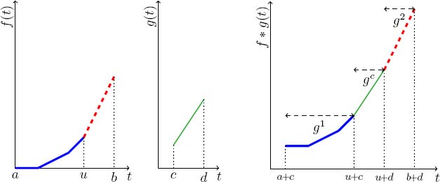
Figure 4.5. Convolution of a convex function by a linear function and decomposition into three functions. For a color version of this figure, see www.iste.co.uk/bouillard/calculus.zip
In other words, g1 is composed of the segments of ![]() whose slope is strictly less than that of g, gc corresponds to the segment g and g2 is composed of the segments of
whose slope is strictly less than that of g, gc corresponds to the segment g and g2 is composed of the segments of ![]() , whose slope is greater than or equal to that of g. Note that gc is also concave.
, whose slope is greater than or equal to that of g. Note that gc is also concave.
Now, suppose that g : [c, d] → ![]() is a concave piecewise linear function represented by the list of segments gj : [cj ,cj+1] →
is a concave piecewise linear function represented by the list of segments gj : [cj ,cj+1] → ![]() , j ∈ [1, m]. Then, by distributivity (Lemma 2.1), and as
, j ∈ [1, m]. Then, by distributivity (Lemma 2.1), and as ![]() ,
,
Let us study where the segments ![]() are placed. The following lemma, which considers two consecutive segments of g, leads to an efficient algorithm to compute the convolution of a convex function by a concave function.
are placed. The following lemma, which considers two consecutive segments of g, leads to an efficient algorithm to compute the convolution of a convex function by a concave function.
LEMMA 4.1.– Consider the convolutions ![]() * gj-1 and
* gj-1 and ![]() * gj. Let
* gj. Let
and
Then:
- –
 ;
; - –
 .
.
PROOF.– First, as ![]() is convex and
is convex and ![]() , we have uj-1
, we have uj-1 ![]() uj. From the above section, for all t
uj. From the above section, for all t ![]() cj + uj,
cj + uj,
Either t ![]() cj-1 + uj-1, then
cj-1 + uj-1, then ![]() * gj-1 (t) =
* gj-1 (t) = ![]() (t - cj-1) + g(cj-1) and
(t - cj-1) + g(cj-1) and
as t – cj–1 ![]() uj-1, the derivative of
uj-1, the derivative of ![]() at t - cj-1 is less than
at t - cj-1 is less than ![]() , so
, so ![]() (t - cj-1) -
(t - cj-1) - ![]() (t - cj)
(t - cj) ![]()
![]() .(cj - cj-1) and
.(cj - cj-1) and ![]() * gj(t) -
* gj(t) - ![]() * gj-1(t)
* gj-1(t) ![]() 0;
0;
or t > cj-1 + uj-1, then ![]() * gj-1(t) =
* gj-1(t) = ![]() (uj-1) + g(t - uj-1). As cj-1 < t - uj-1
(uj-1) + g(t - uj-1). As cj-1 < t - uj-1 ![]() t - uj
t - uj ![]() cj, we have g(cj) - g(t - uj-1) =
cj, we have g(cj) - g(t - uj-1) = ![]() . (cj + uj-1 - t). Moreover, by definition of uj-1, the derivative of
. (cj + uj-1 - t). Moreover, by definition of uj-1, the derivative of ![]() before uj-1 is less than
before uj-1 is less than ![]() and
and ![]() (uj-1) -
(uj-1) - ![]() (t - cj)
(t - cj) ![]()
![]() .(cj + uj-1 - t), so finally,
.(cj + uj-1 - t), so finally, ![]() * gj(t) -
* gj(t) - ![]() * gj-1(t)
* gj-1(t) ![]() 0.
0.
The second statement can be proved similarly.
□
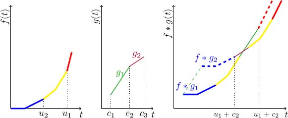
Figure 4.6. Convolution of a convex function by a concave function. For a color version of this figure, see www.iste.co.uk/bouillard/calculus.zip
Another formulation of Lemma 4.1 is that ![]() and
and ![]() , and that the two functions intersect at least once. Hence,
, and that the two functions intersect at least once. Hence, ![]() and
and ![]() cannot appear in the minimum of
cannot appear in the minimum of ![]() * gj and
* gj and ![]() * gj-1. By transitivity, there is no need to compute entirely the convolution of the convex function by every linear component of the decomposition of the concave function. If there are more than two segments, successive applications of this lemma show that only the position of the segments of the concave function has to be computed, except for the extremal segments.
* gj-1. By transitivity, there is no need to compute entirely the convolution of the convex function by every linear component of the decomposition of the concave function. If there are more than two segments, successive applications of this lemma show that only the position of the segments of the concave function has to be computed, except for the extremal segments.
The intersection of ![]() * gj-1 and
* gj-1 and ![]() * gj can then happen in one and only one of the four cases:
* gj can then happen in one and only one of the four cases:
- 1)
 and
and  intersect;
 - 2) and
 intersect;
 - 3)
 and intersect;
 - 4) and intersect.
As a direct consequence of this lemma, a more precise shape of the convolution of a convex function by a concave function can be deduced.
THEOREM 4.2 (Convolution of a convex function by a concave function).– The convolution of a convex function by a concave function can be decomposed in three (possibly trivial) parts: a convex function, a concave function and a convex function.
A formal proof of those result can be found in [BOU 16a]. The main idea is to proceed by induction using Lemma 4.1 for the initialization.
If the concave function is composed of m segments and the convex function of n segments, then the convolution of those two functions can be computed in time ![]() (n + m log m). The log m term comes from the fact that we have to compute the minimum of m segments (see [BOU 08c] for more details).
(n + m log m). The log m term comes from the fact that we have to compute the minimum of m segments (see [BOU 08c] for more details).
Note that the shape of the function is simplified when the functions have infinite supports (b = +∞ or d = +∞). Indeed, either the last slope of ![]() is less than the last slope of g, in which case each slope of
is less than the last slope of g, in which case each slope of ![]() is smaller than each slope of g and
is smaller than each slope of g and ![]() * g =
* g = ![]() + g(0) (assuming without loss of generality that a = c = 0); or the last slope of g is less than the last slope of
+ g(0) (assuming without loss of generality that a = c = 0); or the last slope of g is less than the last slope of ![]() , in which case
, in which case ![]() * g is composed of a convex function and a concave function only, as the convolution by the last segment of g does not make a final convex part appear.
* g is composed of a convex function and a concave function only, as the convolution by the last segment of g does not make a final convex part appear.
4.3. A stable class of functions
The previous section was devoted to simple but limited classes of functions, where some operations can be efficiently implemented.
Unfortunately, it is necessary to define these operations under more general settings. Indeed, convex and concave functions are not stable under every operation, and it is also useful and accurate to deal with more general function, such as periodic functions (e.g. staircase functions).
In this section, we give algorithms for a larger class of functions. This class of function must satisfy two properties:
- 1) stability under all of the operations that we will be using: minimum, maximum, addition, subtraction, (min,plus) convolution, (min,plus) deconvolution and sub-additive closure;
- 2) finitely represented so that the operations can be implemented.
Of course, we would like the class to be as simple as possible. In the following sections, we will define such a class, and first give examples that explain why this class is not that simple. A precise study of those algorithms can be found in [BOU 08c] and, in this chapter, we first review the main results of this article.
4.3.1. Examples of instability of some classes of functions
In section 4.1, numerous classes of functions have been defined. We here justify through example why they had to be defined. As we want a simple and finitely representable class, it is therefore natural to focus on piecewise linear functions that ultimately have a periodic behavior. Indeed, those functions can be represented by a finite sequence of points and slopes. This section enumerates some examples of classes of functions that are not stable. More counterexamples can be found in [BOU 07a]. This section also justifies the class of functions we defined at the beginning of section 4.1.
Linear functions are not stable. The class of linear functions is of course not stable. For example, consider t ![]() min(3t, 5t - 2).
min(3t, 5t - 2).
Ultimately linear functions are not stable. Consider
Then,
where n ∈ ![]() and t ∈ [0,2). Clearly
and t ∈ [0,2). Clearly ![]() is ultimately pseudo-periodic, but not ultimately linear.
is ultimately pseudo-periodic, but not ultimately linear. ![]() and
and ![]() are represented in Figure 4.7.
are represented in Figure 4.7.
These two examples show that we have to choose sets of functions that are large enough. The next examples show that we have to restrict the space of functions we want to consider for a further analysis.
Piecewise linear functions are not stable. Consider a function h defined on [0,1) that is convex and ![]() on this interval (continuous and with a continuous derivative). We will build two piecewise linear functions
on this interval (continuous and with a continuous derivative). We will build two piecewise linear functions ![]() and g such that
and g such that ![]() , showing that piecewise linear functions are not stable.
, showing that piecewise linear functions are not stable.
As h is convex on [0,1), for all t ∈ [0,1), h(t) can be expressed as
by density of ![]() in
in ![]() . As [0, 1) ∩
. As [0, 1) ∩ ![]() is denumerable, there exists a sequence
is denumerable, there exists a sequence ![]() that enumerates all of those elements. We now consider this sequence to construct
that enumerates all of those elements. We now consider this sequence to construct ![]() and g such that
and g such that ![]() .
.

Figure 4.7. Ultimately linear functions are not stable by the sub-additive closure. For a color version of this figure, see www.iste.co.uk/bouillard/calculus.zip
For n ∈ ![]() , set
, set ![]() if t ∈ [0,1) and = –∞ otherwise and gn(2n + t) =
if t ∈ [0,1) and = –∞ otherwise and gn(2n + t) = ![]() if t ∈ [0,1) and = +∞ otherwise. Note that for t ∈ [0,1),
if t ∈ [0,1) and = +∞ otherwise. Note that for t ∈ [0,1),
Define ![]() and
and ![]() . For all t ∈ [0,1),
. For all t ∈ [0,1), ![]() . But, as t ∈ [0,1), it also holds that
. But, as t ∈ [0,1), it also holds that
Figure 4.8 illustrates this construction. Here, we have used functions that take infinite values. In [BOU 07a], it is proved that ![]() and g can be chosen finite and non-decreasing.
and g can be chosen finite and non-decreasing.
To avoid this problem, we will restrict to the class of functions that are ultimately pseudo-periodic and piecewise linear. This way, every function has only a finite number of slopes, and such a construction becomes impossible.

Figure 4.8. A  function from the deconvolution of piecewise linear functions. For a color version of this figure, see www.iste.co.uk/bouillard/calculus.zip
Ultimately pseudo-periodic linear functions are not stable. It is a classical result: if ![]() and g are two periodic functions,
and g are two periodic functions, ![]() + g is periodic if and only if
+ g is periodic if and only if ![]() and g have periods
and g have periods ![]() and
and ![]() with
with ![]() . Therefore, we will only consider piecewise linear functions that only have discontinuities at rational coordinates and rational slopes.
. Therefore, we will only consider piecewise linear functions that only have discontinuities at rational coordinates and rational slopes.
Non-plain functions are not stable. Finally, we also have to consider plain functions. Indeed, if functions are not plain, it is possible to construct functions that are not ultimately periodic. For example, consider ![]() and
and ![]() if there exists n ∈
if there exists n ∈ ![]() , such that t ∈ [2n, 2n + 1] and +∞ otherwise. Thus, min(
, such that t ∈ [2n, 2n + 1] and +∞ otherwise. Thus, min(![]() , g) is not periodic as depicted in Figure 4.9.
, g) is not periodic as depicted in Figure 4.9.
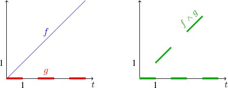
Figure 4.9. Periodic non-plain functions are not stable. For a color version of this figure, see www.iste.co.uk/bouillard/calculus.zip
4.3.2. Class of plain piecewise linear ultimately pseudo-periodic functions
In this section, we show that the class of plain ultimately pseudo-periodic functions in ![]() is stable. As these functions can be finitely represented, it is possible to algorithmically define the (min,plus) operators on these functions. For this, we first propose a data structure to represent them.
is stable. As these functions can be finitely represented, it is possible to algorithmically define the (min,plus) operators on these functions. For this, we first propose a data structure to represent them.
4.3.2.1. Data structure
Let f be a plain ultimately pseudo-periodic function of ![]() . We consider the minimum decomposition into spots, a segment whose support is a singleton, and open segments, whose support is an open interval of
. We consider the minimum decomposition into spots, a segment whose support is a singleton, and open segments, whose support is an open interval of ![]() . Outside of their support, segments are assumed to take value
. Outside of their support, segments are assumed to take value ![]() there exists
there exists ![]()
![]() such that
such that ![]() . Moreover, as f is ultimately periodic, there exists
. Moreover, as f is ultimately periodic, there exists ![]() and
and ![]() such that
such that ![]() and
and ![]() for all
for all ![]() . Hence, it is possible to represent this function f with a finite set of segments and points. More precisely, every spot and open segment
. Hence, it is possible to represent this function f with a finite set of segments and points. More precisely, every spot and open segment ![]() is represented by a quadruplet
is represented by a quadruplet ![]() , where
, where ![]() represents the slope of
represents the slope of ![]() and only the quadruplet corresponds to the transient part and one period is stored. To reconstruct the periodic part of the function, it suffices to store the rank T, period df and increment cf of the function (hf can be deduced from them).
and only the quadruplet corresponds to the transient part and one period is stored. To reconstruct the periodic part of the function, it suffices to store the rank T, period df and increment cf of the function (hf can be deduced from them).
The size of the representation of a function f is denoted by ![]() and is the number of quadruplets used to represent it. Note that this size strongly depends on the choice of T, hence the notation. However, we write Nf the size of the smallest representation of f when
and is the number of quadruplets used to represent it. Note that this size strongly depends on the choice of T, hence the notation. However, we write Nf the size of the smallest representation of f when ![]() , the rank of f. We will have to extend the function beyond the rank to perform the operations.
, the rank of f. We will have to extend the function beyond the rank to perform the operations.
To simplify the proofs of stability, we also use the decomposition of a function f into its transient part ft and its periodic part ![]() , and ft is defined by
, and ft is defined by ![]() and fp on
and fp on ![]() .
.
For the sake of simplicity and without loss of generality, we also assume that the periods of the functions are integers: as they are assumed rational, it suffices to rescale the abscissa.
4.3.2.2. Main theorem and ideas for the algorithms
THEOREM 4.3.– The class of the plain ultimately pseudo-periodic functions of ![]() is stable by the operations of minimum, maximum, addition, subtraction, deconvolution and sub-additive closure.
is stable by the operations of minimum, maximum, addition, subtraction, deconvolution and sub-additive closure.
The rest of the section sketches the proof of this theorem. A complete proof can be found in [BOU 08c].
Consider f and g, plain ultimately pseudo-periodic functions of ![]() . It is obvious that the combination of two plain functions is plain, and we will not prove these.
. It is obvious that the combination of two plain functions is plain, and we will not prove these.
Addition, subtraction of functions
LEMMA 4.2.– ![]() is plain ultimately periodic from
is plain ultimately periodic from ![]() , with period
, with period ![]() and increment
and increment ![]() .
.
PROOF.– ![]() ,
,

using the classical equality ![]() . The subtraction is similar.
. The subtraction is similar.
□
The addition can be done in time ![]() . Indeed,
. Indeed, ![]() . Moreover,
. Moreover, ![]() and
and ![]() . Therefore, it is sufficient to compute addition on the interval [0, T] with
. Therefore, it is sufficient to compute addition on the interval [0, T] with ![]() . One way to compute f + g is to merge the list of spots in [0, T] and compute the addition at each spot as well as the slope between two spots. It can be done through a single pass over f and g. The complexity of this algorithm is
. One way to compute f + g is to merge the list of spots in [0, T] and compute the addition at each spot as well as the slope between two spots. It can be done through a single pass over f and g. The complexity of this algorithm is ![]() .
.
The subtraction can be done the same way.
Minimum, maximum of functions
LEMMA 4.3.– ![]() is plain ultimately periodic, and:
is plain ultimately periodic, and:
- – if
 , then ultimately,
  with period df and increment cf;
 - – if
 , then ultimately,
  with period dg and increment cg;
 - – if
 , then
  is ultimately periodic from
  with period
  and increment
  .
.
PROOF.– The first two cases are symmetric, so we focus on the first and third ones. Set ![]() , and
, and ![]() . In the third case, for all
. In the third case, for all ![]() ,
,
In the first case, there exists ![]() such that, for all
such that, for all ![]()
![]() , and there exists
, and there exists ![]() such that, for all
such that, for all ![]() , and by hypothesis,
, and by hypothesis, ![]() . Therefore, from
. Therefore, from ![]() ,
,
so ![]() , and the rest follows.
, and the rest follows.
□
As shown in the proof, in case the two functions do not have the same growth rate, it is not easy to compute in advance the rank from which ![]() is pseudo-periodic (the proof only gives an upper bound). Algorithmically, the solution is to go through the quadruplets of functions f and g in order, computing the intersection of segments, and extending the functions from one period at a time when the transient period or a function has been treated. When the minimum is
is pseudo-periodic (the proof only gives an upper bound). Algorithmically, the solution is to go through the quadruplets of functions f and g in order, computing the intersection of segments, and extending the functions from one period at a time when the transient period or a function has been treated. When the minimum is ![]() on a complete period of f (or g), let us say from time T,
on a complete period of f (or g), let us say from time T, ![]() has become pseudo-periodic. The complexity is then in
has become pseudo-periodic. The complexity is then in ![]() .
.
Convolution offunctions
LEMMA 4.4.– f ∗ g is ultimately pseudo-periodic with period ![]() and increment
and increment ![]() .
.
PROOF.– We use the decomposition of f and g into their transient and periodic parts:
As ft and gt have a finite support, so does ![]() , which is then ultimately equal to
, which is then ultimately equal to ![]() .
.
Let us now focus on ![]() . For all
. For all ![]()
![]() . Owing to the support of ft, s can be taken to not be greater than Tf, so
. Owing to the support of ft, s can be taken to not be greater than Tf, so ![]() , so
, so ![]() and
and ![]() is ultimately pseudo-periodic with period dg and increment cg. Similarly,
is ultimately pseudo-periodic with period dg and increment cg. Similarly, ![]() is ultimately pseudo-periodic with period df and increment Cf.
is ultimately pseudo-periodic with period df and increment Cf.
Finally, let us show that ![]() is pseudo-periodic. For all
is pseudo-periodic. For all ![]() ,
,
f ∗ g is then the minimum of four ultimately periodic functions of ![]() , so it is itself ultimately pseudo-periodic from Lemma 4.3.
, so it is itself ultimately pseudo-periodic from Lemma 4.3.
□
Algorithmically, a generic way of computing the convolution of a function is to compute the convolution of each pair of segments of f and g. The (min,plus) convolution of two segments is a direct consequence of Theorem 4.1: a segment is convex. Just note that this result holds for open segments. The convolution of two segments can be made in constant time, and then, by distributivity of the convolution over the minimum, the minimum of all these convolutions has to be computed. Using Lemma 4.3, it is possible to compute the rank T from which f ∗ g will be ultimately periodic. The number of segment convolutions to compute is then in ![]() , and the minimum of all these functions has to be computed. The use of a divide-and-conquer approach leads to a
, and the minimum of all these functions has to be computed. The use of a divide-and-conquer approach leads to a ![]() complexity.
complexity.
It is also possible, if it makes sense, to use the shape of the function, and decompose it into convex and concave parts in order to use efficient convolution algorithms from Theorems 4.1 and 4.2.
Deconvolution offunctions
LEMMA 4.5.– ![]() is ultimately pseudo-periodic from Tf with period df and increment cf.
is ultimately pseudo-periodic from Tf with period df and increment cf.
PROOF.-For all ![]() ,
,
□
To compute the deconvolution of two functions f and g, we also use the properties of the deconvolution of Propositions 2.7 and 2.8 ![]()
![]() and the following lemma for the convolution of segments.
and the following lemma for the convolution of segments.
LEMMA 4.6.– Let ![]() and
and ![]() be two segments, respectively, defined on the intervals I and J. Let a = inf I and d = sup J. Then,
be two segments, respectively, defined on the intervals I and J. Let a = inf I and d = sup J. Then, ![]() is defined on
is defined on ![]()
![]() and consists of concatenating the segments f and g from
and consists of concatenating the segments f and g from ![]() , with the segment with the larger slope first, where
, with the segment with the larger slope first, where ![]() .
.
Note that, in this lemma, outside J, we set by default ![]() .
.
PROOF.– First, ![]() is defined if
is defined if ![]() and finite if there exists
and finite if there exists ![]() such that
such that ![]() . We use the additional notations b = sup I and c = inf J, and recall that
. We use the additional notations b = sup I and c = inf J, and recall that ![]() is the slope of f (resp g).
is the slope of f (resp g).
Either ![]() , and u has to be maximized, if
, and u has to be maximized, if ![]()
![]() and if
and if ![]() or
or ![]() , and u has to be minimized: if
, and u has to be minimized: if ![]() , and if
, and if ![]() .
.
□
Similarly to the convolution, we decompose the functions into segments and spots and perform the elementary deconvolutions on these, and compute the maximum of these.
Sub-additive closure of a function
Computing the sub-additive closure of a function is more complex. The following lemma gives a trick to compute only the sub-additive closure as a finite number of convolutions of segments and spots. This result is unpublished and credited to Sébastien Lagrange.
LEMMA 4.7.– Let ![]() . Then,
. Then, ![]() .
.
PROOF.– Recall that ![]() is the unit element of the dioid of (min,plus) functions. From Proposition 2.6,
is the unit element of the dioid of (min,plus) functions. From Proposition 2.6, ![]() and
and ![]() for all
for all ![]() . Therefore, by commutativity of the (min,plus) convolution,
. Therefore, by commutativity of the (min,plus) convolution,
□
We can now apply the lemma by slightly modifying the representation of a function f. We still have ft as its transient part, but we decompose the periodic part into ![]()
![]() , where f1p is the restriction of f to
, where f1p is the restriction of f to ![]() (it is only the first period), and fs is a spot defined at
(it is only the first period), and fs is a spot defined at ![]() . Therefore, f can be expressed as
. Therefore, f can be expressed as ![]() . From Lemma 4.7,
. From Lemma 4.7, ![]() . Only the sub-additive closure of functions composed of a finite number of spots and segments has to be computed, which boils down to computing the sub-additive closure of spots and segments (using
. Only the sub-additive closure of functions composed of a finite number of spots and segments has to be computed, which boils down to computing the sub-additive closure of spots and segments (using ![]() .
.
LEMMA 4.8.– Let f be a spot: f is defined on {d} and f (d) = c. Then, f * is a function defined on ![]() and f (nd) = nc for all
and f (nd) = nc for all ![]() .
.
PROOF.– For all ![]() , fn is a spot defined at nd and
, fn is a spot defined at nd and ![]() , so the result straightforwardly holds since
, so the result straightforwardly holds since ![]() .
.
□
LEMMA 4.9.– If f is a segment defined on an open interval, then f * is ultimately pseudo-periodic.
PROOF.– Suppose that f is defined on (a, b) and that ![]() for all
for all ![]() . For all
. For all ![]() , fn is an open segment of slope f' defined on (na, nb). We differentiate two cases, depending on how f'a compares to f (a).
, fn is an open segment of slope f' defined on (na, nb). We differentiate two cases, depending on how f'a compares to f (a).
First, assume that ![]() . This is equivalent to
. This is equivalent to ![]() . Let
. Let ![]() . Then, f * is ultimately pseudo-periodic from n0b, of period b and increment f 'b: for all
. Then, f * is ultimately pseudo-periodic from n0b, of period b and increment f 'b: for all ![]()
wherever ![]() is defined, that is, for t > b. Therefore, if
is defined, that is, for t > b. Therefore, if ![]()
![]() .
.
If ![]() , then f * is ultimately pseudo-periodic from n0a, of period a and increment f 'a: for all
, then f * is ultimately pseudo-periodic from n0a, of period a and increment f 'a: for all ![]() ,
,
Therefore, for ![]() .
.
□
The sub-additive closure is algorithmically the most costly operator: it is even an NP-hard problem to know the rank from which a function is pseudo-periodic: considering a function that is 0 everywhere except at a finite set ![]() , it is equivalent to solve the Frobenius problem:
, it is equivalent to solve the Frobenius problem: ![]()
![]() , which is proved to be NP-hard in [RAM 96].
, which is proved to be NP-hard in [RAM 96].
4.3.3. Functions with discrete domain
We discussed our choice of using ![]() as the time domain in section 1.3. Indeed, there is in general no assumption of a common clock synchronizing a network. However, for some applications where a synchronizing clock exists, such as systems-on-chip, it may be more accurate to use the time domain
as the time domain in section 1.3. Indeed, there is in general no assumption of a common clock synchronizing a network. However, for some applications where a synchronizing clock exists, such as systems-on-chip, it may be more accurate to use the time domain ![]() .
.
Let ![]() denote the set of functions of a discrete time domain. All the (min,plus) operators can be defined similarly to the continuous case, and are denoted
denote the set of functions of a discrete time domain. All the (min,plus) operators can be defined similarly to the continuous case, and are denoted ![]() . For example,
. For example, ![]()
![]() .
.
From an algebraic viewpoint, the associativity, commutativity and distributivity properties of the (min,plus) operators remain, so that ![]() is a dioid. Some properties are even simpler to obtain, as, for example, the (min,plus) convolution is now computed as a minimum and not an infimum.
is a dioid. Some properties are even simpler to obtain, as, for example, the (min,plus) convolution is now computed as a minimum and not an infimum.
It is also possible to link the results of the operators in the continuous-time domain and the discrete-time domain. For this, we must first define projection and interpolation between the two domains. For ![]() , we denote by
, we denote by ![]() its projection on
its projection on ![]() .
.
Conversely, different interpolations, illustrated in Figure 4.10, from ![]() can be defined:
can be defined:
- 1) the linear interpolation
 ;
; - 2) the left-continuous staircase function
 ;
; - 3) the right-continuous staircase function
 .
.
We now can make explicit the relations between the projections and interpolations.
First, it was shown in [BOU 08c, Prop. 1] that for any operator ![]() and any function
and any function ![]() ,
,
and in [BOU 07b, Prop. 2] that if, moreover, f is non-decreasing,
Note that these equalities only hold for expressions involving one single operator: for more complex expressions, performing all computations in the continuous-time domain from the interpolated functions and then going back to the discrete-time domain may not lead to the right result. An example is ![]() : as a function in
: as a function in ![]() , we have f (3) = 6, but as a function in
, we have f (3) = 6, but as a function in ![]() , we have f (3) = 7.
, we have f (3) = 7.

Figure 4.10. Three projections from discrete to dense time domain
From an algorithmic viewpoint, the choice of the time domain strongly depends on the shape of the functions: if the linear interpolation reduces the size of the representation, it might be efficient to use it. Otherwise, a discrete-time representation might be more efficient. The algorithms can easily be adapted to the discrete-time domain.
4.4. Containers of (min,plus) functions
In section 4.3, the class of plain piecewise linear ultimately pseudo-periodic functions is defined such that they are stable for the operations of network calculus (see Theorem 4.3). However, the exact computations of the minimum ![]() , the convolution ∗ and the sub-additive closure .* can be really time- and memory-consuming, especially when the growth rate of the functions are very close to each other.
, the convolution ∗ and the sub-additive closure .* can be really time- and memory-consuming, especially when the growth rate of the functions are very close to each other.
Let f and g be two plain piecewise linear ultimately pseudo-periodic functions such that ![]() with the rank
with the rank ![]() , and
, and ![]() with the rank
with the rank ![]() . The inf-convolution h = f ∗ g is a plain piecewise linear ultimately pseudo-periodic function with Th = 496 (g(Th) = 473). There are 253 segments before the periodic part of h because the inf-convolution needs this time to decide which function is really above the other.
. The inf-convolution h = f ∗ g is a plain piecewise linear ultimately pseudo-periodic function with Th = 496 (g(Th) = 473). There are 253 segments before the periodic part of h because the inf-convolution needs this time to decide which function is really above the other.
Therefore, here, we propose not to deal with exact computations but with operations called inclusion functions. The results of these operations are particular intervals called containers and they contain in a guaranteed way the results obtained with exact computations.
More precisely, inclusion functions are defined both in order to contain the result of the exact computations in a guaranteed way, and to be less time- and memory-consuming than the exact computations. It is obvious that it intrinsically adds pessimism compared to exact computations. However, inclusion functions are proposed with interesting algorithm complexity and small storage capacity for the data structures, and they allow us to obtain containers that are as small as possible.
REMARK 4.1.– The work of this section is introduced in [LEC14] with a strong connection to the dioid algebraic structure. For instance, notation ⊕ and terms sum or addition are used instead of notation ∧ and term minimum. Moreover, a strong modification is that the dioid order relation ![]() is used instead of the natural order. This means that all of the notations have to be inverted between this section and that paper.
is used instead of the natural order. This means that all of the notations have to be inverted between this section and that paper.
4.4.1. Notations and context
All functions of this section belong to ![]() , the set of non-negative and non-decreasing functions. Remember that
, the set of non-negative and non-decreasing functions. Remember that ![]() is a complete dioid.
is a complete dioid.
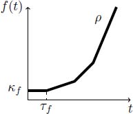
Figure 4.11. A convex function 
Furthermore, the bounds of the containers are piecewise linear and ultimately linear. Among these functions, convex functions – with a constant part on ![]() (see Figure 4.11) - and almost concave functions – almost because they are constant on the interval
(see Figure 4.11) - and almost concave functions – almost because they are constant on the interval ![]() and concave on
and concave on ![]() (see Figure 4.12) – are used. Convex functions belong to the set that we denote as
(see Figure 4.12) – are used. Convex functions belong to the set that we denote as ![]() , and almost concave functions to the set that we denote as
, and almost concave functions to the set that we denote as ![]() . The asymptotic slope of a function
. The asymptotic slope of a function ![]() is the slope of the last semi-infinite segment denoted
is the slope of the last semi-infinite segment denoted ![]() . This slope cannot be infinite.
. This slope cannot be infinite.

Figure 4.12. A function  that is concave on
A function of either ![]() can be seen as the following convolution:
can be seen as the following convolution:

where function ![]() is called an elementary function and is defined by:
is called an elementary function and is defined by:
This means that these convex and almost concave functions can always be reduced to a piecewise linear convex or concave function, null at the origin and shifted in the plane by an elementary function. Function g can also be expressed as ![]() .
.
During the computations, we will also need some approximation operators in order to always bring back the results in sets ![]() and
and ![]() . Let
. Let ![]() be a non-decreasing function of
be a non-decreasing function of ![]() . On the one hand,
. On the one hand, ![]() is the convex hull of
is the convex hull of ![]() , i.e. the greatest convex function smaller than
, i.e. the greatest convex function smaller than ![]() . Hence,
. Hence, ![]() . On the other hand,
. On the other hand, ![]() is the concave approximation defined as follows:
is the concave approximation defined as follows:
where ![]() and
and ![]() is the smallest concave function greater than
is the smallest concave function greater than ![]() on
on ![]() . Hence,
. Hence, ![]() .
.
Finally, ![]() (respectively
(respectively ![]() ) if
) if ![]() is an ultimately linear function, and
is an ultimately linear function, and ![]() (respectively
(respectively ![]() ) if
) if ![]() is an ultimately pseudo-periodic function with growth rate
is an ultimately pseudo-periodic function with growth rate ![]() .
.
4.4.2. The object container
In this section, we use the Legendre–Fenchel transform ![]() introduced in section 3.3.2, and
introduced in section 3.3.2, and ![]() is the set of functions that have the same Legendre–Fenchel transform as
is the set of functions that have the same Legendre–Fenchel transform as ![]() .
.
DEFINITION 4.2 (Set F of containers).– The set of containers is denoted by F and defined by
with ![]() the subset is defined as
the subset is defined as
Hence, a container of F is a subset of an interval ![]() , the bounds of which are convex for
, the bounds of which are convex for ![]() , are almost concave for
, are almost concave for ![]() and have the same asymptotic slope
and have the same asymptotic slope ![]() . A container of F is also a subset of an equivalent class
. A container of F is also a subset of an equivalent class ![]() . This means that all elements of
. This means that all elements of ![]() are equivalent to
are equivalent to ![]() modulo the Legendre–Fenchel transform
modulo the Legendre–Fenchel transform ![]() .
.
Properties of the lower bound
The lower bound ![]() plays a very important role in the definition of a container thanks to the following proposition:
plays a very important role in the definition of a container thanks to the following proposition:
PROPOSITION 4.2.– Functions ![]() , g ∈
, g ∈ ![]() have the same Legendre–Fenchel transform if and only if they have the same convex hull:
have the same Legendre–Fenchel transform if and only if they have the same convex hull:
Moreover, the convex hull of ![]() is the least representative of
is the least representative of ![]() :
:
PROOF.– First, ![]() and
and ![]() is an isotone mapping, so
is an isotone mapping, so ![]() (from Proposition 3.15 because
(from Proposition 3.15 because ![]() is a convex function). But
is a convex function). But ![]() is the greatest convex function smaller than
is the greatest convex function smaller than ![]() and
and ![]() is convex, so
is convex, so ![]() . Thus,
. Thus, ![]() .
.
Now, we deduce ![]() .
.
Conversely, ![]() is convex, so
is convex, so ![]() . Therefore,
. Therefore, ![]() .
.
The second part of the proposition is equivalent to equation [3.14].
□
This proposition allows us to say that because ![]() , we have
, we have ![]() which is equal to
which is equal to ![]() . Consequently, for a function
. Consequently, for a function ![]() ∈
∈ ![]() , the non-differentiable points of
, the non-differentiable points of ![]() truly belong to
truly belong to ![]() . They also have the same asymptotic slope (or growth rate). Moreover, we can see that
. They also have the same asymptotic slope (or growth rate). Moreover, we can see that ![]() is the least representative of
is the least representative of ![]() and so of
and so of![]() .
.
Equivalence class ![]() is graphically illustrated in Figure 4.13 by the gray zone. Functions that have the same non-differentiable points and the same asymptotic slope as
is graphically illustrated in Figure 4.13 by the gray zone. Functions that have the same non-differentiable points and the same asymptotic slope as ![]() (which is an ultimately pseudo-periodic function in this figure) belong to this equivalent class for which
(which is an ultimately pseudo-periodic function in this figure) belong to this equivalent class for which ![]() is the least representative.
is the least representative.
Figure 4.13. Equivalence class 
Finally, the following proposition says that equivalence classes modulo the Legendre–Fenchel transform are actually elements of a dioid.
PROPOSITION 4.3 (Dioid ![]() ).– The quotient of dioid
).– The quotient of dioid ![]() by congruence
by congruence ![]() (defined in equation 3.13) provides another dioid denoted as
(defined in equation 3.13) provides another dioid denoted as ![]() . Elements of
. Elements of ![]() are equivalence classes modulo the Legendre–Fenchel transform
are equivalence classes modulo the Legendre–Fenchel transform ![]() . Minimum and convolution between them are such that:
. Minimum and convolution between them are such that:
By deduction, sub-additive closure of ![]() is such that:
is such that:
PROOF.–From Proposition 3.15, ![]() . Therefore, if
. Therefore, if ![]() and
and ![]() , then
, then ![]() . So
. So ![]() and
and ![]() and
and ![]() is well defined.
is well defined.
The same considerations apply to the convolution and to the sub-additive closure.
□
As a result of this proposition, performing computations on the lower bounds of containers actually amounts to use operations of the dioid ![]() and to handle canonical representatives (the least ones) of its elements, since the elements of
and to handle canonical representatives (the least ones) of its elements, since the elements of ![]() are equivalent to
are equivalent to ![]() modulo the Legendre–Fenchel transform
modulo the Legendre–Fenchel transform ![]() .
.
In addition, the following lemma provides some nice equivalences that will be used for the computations between containers. They directly follow from Propositions 4.2 and 4.3.
LEMMA 4.10.– Computing with elements of dioid ![]() is equivalent to computing with convex hulls of functions. Formally,
is equivalent to computing with convex hulls of functions. Formally, ![]() :
:
Canonical representation
Now, by defining a canonical upper bound of ![]() and because
and because ![]() is the canonical lower bound of a container, it is possible to obtain a canonical representation of a container as follows:
is the canonical lower bound of a container, it is possible to obtain a canonical representation of a container as follows:
PROPOSITION 4.4 (Canonical upper bound of ![]() ).– Let
).– Let ![]() be an equivalence class modulo the Legendre–Fenchel transform and
be an equivalence class modulo the Legendre–Fenchel transform and ![]() be its least element, i.e.
be its least element, i.e. ![]() . The piecewise constant function
. The piecewise constant function ![]() defined below as the sum of elementary functions is a canonical upper bound of
defined below as the sum of elementary functions is a canonical upper bound of ![]() :
:
where pairs (ti,ki) are the coordinates of the non-differentiable points of ![]() . Therefore:
. Therefore:
This upper bound is illustrated by the bold segments in Figure 4.14 in which the gray zone represents the equivalent class ![]() .
.
Figure 4.14. Upper bound  of the equivalent class
It must be noted that ![]() does not belong to
does not belong to ![]() since the asymptotic slope of
since the asymptotic slope of ![]() , i.e. +∞, is not equal to the asymptotic slope of
, i.e. +∞, is not equal to the asymptotic slope of ![]() , the least element of
, the least element of ![]() .
.
DEFINITION 4.3 (Canonical representation of a container).– The canonical representation of a container ![]() is
is
Note that with this representation, with ![]() .
.
The advantage of such a canonical representation is to remove some ambiguities. Indeed, if ![]() ∈
∈ ![]() , then
, then ![]() . Hence, as is illustrated in Figure 4.15,
. Hence, as is illustrated in Figure 4.15, ![]() is the greatest element of the container
is the greatest element of the container ![]() , and interval
, and interval ![]() (the gray zone in Figure 4.15) contains function
(the gray zone in Figure 4.15) contains function ![]() . Consequently, as illustrated in Figure 4.16, the same container of F can be represented by different intervals,
. Consequently, as illustrated in Figure 4.16, the same container of F can be represented by different intervals, ![]() and
and ![]() , as long as
, as long as ![]() .In other words, we can have
.In other words, we can have
In Figure 4.16, this canonical representation is given by the container ![]() since
since ![]() .
.
By conducting the concave approximation of ![]() , we are still in the set F and we propose a canonical representation of objects that we handled.
, we are still in the set F and we propose a canonical representation of objects that we handled.
Data structure. This canonical representation will also be the one chosen as data structure for the function representation. Indeed, in addition to offering the advantage of unambiguously representing a container of F, it allows useless points of ![]() to be removed. In the example of Figure 4.16, the points of
to be removed. In the example of Figure 4.16, the points of ![]() and
and ![]() graphically located above
graphically located above ![]() can thus be removed in order to keep only the canonical representation
can thus be removed in order to keep only the canonical representation ![]() .
.
Figure 4.15. Greatest element  of the container
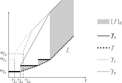
Figure 4.16. Canonical representation  of the identical container
 and
and 
Maximum uncertainty of a container
Due to the canonical representation of a container, the maximal distances in time and data domains between ![]() and
and ![]() are finite and the loss of precision due to approximations is bounded. This uncertainty is defined below with the following precision: abscissa of the last semi-infinite segment of an ultimately linear function
are finite and the loss of precision due to approximations is bounded. This uncertainty is defined below with the following precision: abscissa of the last semi-infinite segment of an ultimately linear function ![]() is the rank of
is the rank of ![]() denoted as
denoted as ![]() , and its corresponding ordinate is
, and its corresponding ordinate is ![]() .
.
DEFINITION 4.4 (Maximal uncertainty of a container f).– Let ![]() be a container of F in its canonical form. Its maximal uncertainty is defined as follows in the time domain (see Figure 4.17):
be a container of F in its canonical form. Its maximal uncertainty is defined as follows in the time domain (see Figure 4.17):

and in the data domain (see Figure 4.18):
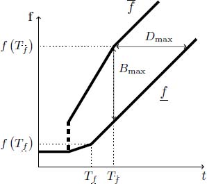
Figure 4.17. Maximal uncertainties  and
and  of a container f ∈ F when
  and
and 

Figure 4.18. Maximal uncertainties  of a container
  when
when  and
and 
4.4.3. Inclusion functions for containers
As stated at the beginning of this section, operations defined for the containers and called inclusion functions must be such that:
- – they contain the result of exact computations in a guaranteed way;
- – they are closed for set F of containers;
- – they can be computed with an interesting algorithm complexity;
- – they provide containers that are as small as possible.
The first two criteria are mathematically proven thanks to the properties of handled functions. In particular, the condition of closure is mainly fulfilled because of the dioid structure of the convex lower bound of a container. The last two criteria are conditions that we impose on definitions to get efficient and interesting results about these computations.
DEFINITION 4.5 (Inclusion functions ![]() ). –Let
). –Let ![]() and
and ![]() be two containers of F given in their canonical forms. Inclusion functions of minimum
be two containers of F given in their canonical forms. Inclusion functions of minimum ![]() and convolution ∗ are denoted as
and convolution ∗ are denoted as ![]() and
and ![]() . They are defined by:
. They are defined by:
Now, let ![]() be a container not necessarily given in its canonical form. Inclusion function of the sub-additive closure .* is denoted as [∗] and defined by:
be a container not necessarily given in its canonical form. Inclusion function of the sub-additive closure .* is denoted as [∗] and defined by:
with

![]() are elementary functions for which pairs (ti,ki) are the non-differentiable points of
are elementary functions for which pairs (ti,ki) are the non-differentiable points of ![]() . Functions
. Functions ![]() are defined in equation [4.4]:
are defined in equation [4.4]: ![]() .
.
In this definition of inclusion functions, the choice of picking either the canonical form of the container or the interval without the concave approximation (i.e. ![]()
![]() ), is relevant in order to obtain a weak level of complexity in all cases.
), is relevant in order to obtain a weak level of complexity in all cases.
Moreover, these inclusion functions do not necessarily provide canonical results. A simple way to obtain them is to make at the end of the computation the concave approximation of the minimum between the obtained upper bound and the actual upper bound of the equivalence class of the lower bound. For instance, the canonical result of ![]() is given by:
is given by:
THEOREM 4.4.–Let ![]() and
and ![]() be two containers of F. Inclusion functions
be two containers of F. Inclusion functions ![]() are such that:
are such that:
PROOF.– The entire proof is given in [LEC 14]. Here, we just give its general idea.
Lower bounds of inclusion functions
We saw that the lower bound of a container is the canonical representative of an element of ![]() , since it is the least element of the equivalence class modulo
, since it is the least element of the equivalence class modulo ![]() . Therefore, operations on elements of
. Therefore, operations on elements of ![]() are closed in dioid
are closed in dioid ![]() and so obtained lower bounds are closed in the set F. In addition, because of equations [4.7]–[4.9], we know that exact computations are included in obtained containers. Indeed, the computations are made with canonical representatives of equivalence classes (the least ones), which means that they are valid for all the other functions of the equivalence classes. Therefore,
and so obtained lower bounds are closed in the set F. In addition, because of equations [4.7]–[4.9], we know that exact computations are included in obtained containers. Indeed, the computations are made with canonical representatives of equivalence classes (the least ones), which means that they are valid for all the other functions of the equivalence classes. Therefore, ![]() and
and ![]() .
.
For the minimum and the sub-additive closure, equations [4.10] and [4.12] correspond exactly to definitions of equations [4.14] and [4.16]. For the convolution, Proposition 3.13 allows us to say that if ![]() , then
, then ![]() so
so ![]() . Hence, we do not need to make the concave approximation given in equation [4.11], but simple to directly perform the computation given in equation [4.15].
. Hence, we do not need to make the concave approximation given in equation [4.11], but simple to directly perform the computation given in equation [4.15].
Upper bounds of inclusion functions
- – For the minimum, according to equation [4.6] about the definition of the concave approximation and since
 is order-preserving, it is obvious that
  and
and  ,
,  , that
  and that
  .
. - – For the convolution, remember that functions of
 can always be factorized (see equation [4.4]). Therefore, we obtain
  with:
and
with:
and
 (because of Proposition 3.12). Then, the minimum of two concave functions that take value 0 at 0, like f ' and g', provides a concave result (again according to Proposition 3.12) and allows us to avoid making the concave approximation of
  . Moreover, the asymptotic slope of
  is equal to that of f[*]g and so to that of f * g. Finally, since * is order preserving,
  and
and  ,
,  .
. - – For the sub-additive closure, it is a little bit more tricky. The general idea is to use the largest element of container f, i.e.
 . Then, through the use of the upper bound
  , non-differentiable points of
  are introduced in the computation, which allow us to be the least pessimistic. The following sub-additive closure is computed:
In these lines, Lemma 2.6 and Proposition 3.12 are used for the equality g = g*; Proposition 2.6 to say that the sub-additive closure of the minimum of functions is equal to the convolution of the sub-additive closures of the functions, and the fact that the sub-additive closure is linked to the Kleene star operator (Theorem 2.3).
Some sub-additive closures of elementary functions appear in the last two lines. Unfortunately, the result of these computations provides ultimately pseudo-periodic functions such that ![]() , and for which the rank is reached at t = 0 with
, and for which the rank is reached at t = 0 with ![]() for the growth rate. The problem is that making convolutions between such functions is not easy in an algorithmic sense. Hence, we propose to make their concave approximations and thus obtain easier functions to compute (i.e. almost concave functions that take value 0 at 0):
for the growth rate. The problem is that making convolutions between such functions is not easy in an algorithmic sense. Hence, we propose to make their concave approximations and thus obtain easier functions to compute (i.e. almost concave functions that take value 0 at 0):
By doing all of these concave approximations, it is obvious that we over-approximate the result we might obtain. However, these over-approximations allow us to compute the minimum of concave functions instead of the convolution that is much better for algorithm complexity. Indeed, thanks to Proposition 3.12, we have the following equality:
which is the computation of ![]() . With this upper bound, we still have
. With this upper bound, we still have ![]() ,
, ![]() ; and
; and ![]() .
.
□
Algorithms and complexities
Now, let us deal with the ideas of algorithms used for the computations of inclusion functions. Let ![]() and
and ![]() be the number of non-differentiable points of
be the number of non-differentiable points of ![]() ,
, ![]() and
and ![]() , respectively. We also call these numbers the sizes of the bounds (instead of the case in section 4.3 where size is for the number of segments). We will see that algorithms are of linear or quasi-linear time of the size of the container bounds.
, respectively. We also call these numbers the sizes of the bounds (instead of the case in section 4.3 where size is for the number of segments). We will see that algorithms are of linear or quasi-linear time of the size of the container bounds.
Minimum
Inclusion function ![]() can be computed in linear time in the size of the bounds of the containers.
can be computed in linear time in the size of the bounds of the containers.
Indeed, the first step of the computation is to make the minimum of the lower bounds ![]() and
and ![]() and of the upper bounds
and of the upper bounds ![]() and
and ![]() . This requires in the worst case only one scan of non-differentiable points of each function, and so can be done in linear time in the size of the bounds.
. This requires in the worst case only one scan of non-differentiable points of each function, and so can be done in linear time in the size of the bounds.
Then, since the minimum of two convex functions is not convex, the minimum of two almost concave functions is neither a concave function nor an almost concave function, and we need to compute the convex hull of ![]() and the concave approximation of
and the concave approximation of ![]() to get a closed result in F. This can also be done in linear time by using well-known algorithms of convex hull computation.
to get a closed result in F. This can also be done in linear time by using well-known algorithms of convex hull computation.
Therefore, the complexity of algorithm that computes inclusion function ![]() is in
is in ![]() .
.
Convolution
Inclusion function [∗] can be computed in linear time in the size of the bounds of the containers.
First, the computation of ![]() is obtained by putting end to end the different linear pieces of
is obtained by putting end to end the different linear pieces of ![]() and
and ![]() , sorted by non-decreasing slopes, up to reach the least asymptotic slope between
, sorted by non-decreasing slopes, up to reach the least asymptotic slope between ![]() and
and ![]() (see Theorem 4.1). Hence, the computation only requires a simple scan of functions1.
(see Theorem 4.1). Hence, the computation only requires a simple scan of functions1.
Second, about the upper bound, the convolution is defined as ![]() . Hence, the minimum between
. Hence, the minimum between ![]() and
and ![]() can be done with a linear complexity and the convolution by the elementary function (that corresponds to a shift in the plane) can be done in a constant time, namely in
can be done with a linear complexity and the convolution by the elementary function (that corresponds to a shift in the plane) can be done in a constant time, namely in ![]() .
.
Therefore, the complexity of algorithm that computes inclusion function [∗] is in ![]()
Sub-additive closure
The algorithm complexity of [∗] is given separately for the two bounds ![]() and
and ![]() .
.
First, the lower bound ![]() is obtained in linear time in the size of
is obtained in linear time in the size of ![]() . Indeed, its computation only requires the research of its asymptotic slope by checking the
. Indeed, its computation only requires the research of its asymptotic slope by checking the ![]() non-differentiable points of
non-differentiable points of ![]() and the asymptotic slope
and the asymptotic slope ![]() . Therefore, the complexity of algorithm that computes
. Therefore, the complexity of algorithm that computes ![]() is in
is in ![]() .
.
Second, the upper bound ![]() is obtained in quasi-linear time. Indeed, the computation of
is obtained in quasi-linear time. Indeed, the computation of ![]() , the first part of equation [4.17], is made thanks to algorithms such as “divide and conquer”. Therefore, by doing a two-by-two minimum of
, the first part of equation [4.17], is made thanks to algorithms such as “divide and conquer”. Therefore, by doing a two-by-two minimum of ![]() , the computation of the n functions is solved in
, the computation of the n functions is solved in ![]() . According to the second part of the equation, the minimum between
. According to the second part of the equation, the minimum between ![]() and g (from
and g (from ![]() ) is made in linear time, namely
) is made in linear time, namely ![]() , where Ng is the number of non-differentiable points of g. Then, the shift of
, where Ng is the number of non-differentiable points of g. Then, the shift of ![]() is in
is in ![]() as well as the minimum with e (the unit element of the dioid). The concave approximation does not modify this result since its computation is in linear time. Thus, the complexity of this part of the equation is in
as well as the minimum with e (the unit element of the dioid). The concave approximation does not modify this result since its computation is in linear time. Thus, the complexity of this part of the equation is in ![]() . Therefore, the complexity of algorithm that computes
. Therefore, the complexity of algorithm that computes ![]() is in
is in ![]() .
.
4.5. Implementations
Several implementations of the algorithmic procedures presented in this chapter have been developed, either as autonomous libraries or part of a network calculus tool. The main implementations are listed in this section. For those included in a tool, only the classes of functions handled are listed here; the tools themselves will be presented in the Conclusion.
- – The DISCO Network Calculator is a network calculus Java tool [DIS 18]. Its principles are detailed in [SCH 06c]. It handles functions made up of a finite prefix followed by a linear tail (i.e. ultimately linear function, see section 4.1). This finite prefix can be any piecewise linear function, i.e. made up of a finite number of linear segments. It handles either floating point or rational numbers.
- – The NC-maude tool is a Maude toolbox [BOY 15]. Its principles are detailed in [BOY 10b], and it uses the Maude rewriting language [MAU 15]. It handles piecewise linear continuous concave and rate-latency functions, with rational numbers.
- – The containers of section 4.4 are implemented in the tool ContainerMinMaxGD [CON 09] developed in C++ language. This tool is an extension to the MinMaxGD library that implements operations over periodic series in dioid of formal series. It is very similar to the classical dioid theory as described in [LEC 14].
- – The real-time calculus (RTC) toolbox is a Matlab® toolbox for performance analysis of distributed real-time and embedded systems [WAN 06a, WAN 06b]. Its Java kernel implements the main network calculus operations, except the sub-additive closure. It deals with piecewise linear functions defined over
 , which are not necessarily increasing nor positive but which have a periodic behavior from a point, called variability characterization curves (VCCs). Infinite values are also allowed. This class is very close to the classes introduced here where this asymptotic behavior is called ultimate pseudo-periodicity. Besides correctness, no complexity analysis has been given as far as we know.
 - – The software COINC [COI 07] was the first to implement the algorithms presented in [BOU 08c], as a standalone version or a Scilab toolbox.
- – The RTaW-PEGASE tool [BOY 10c, BOY 11a] implements three classes of functions. Like DISCO, it implements the piecewise linear concave and convex functions, with either floating point or rational numbers. It also implements the most general class of functions of the ultimately pseudo-periodic function of [BOU 08c], but only with rational numbers (since this class requires us to compute l cm), and does not implement sub-additive closure. Last, it implements a class that groups the stair-shaped functions and the piecewise linear concave and convex functions. Since this class is not closed by common operations, only a subset of operations is defined [BOY 11b].
The (min,+) library can be used either as an API, within a dedicated command-line interpreter, or through a WEB server, at http://realtimeatwork.com/minplus-playground.