
11
Tight Worst-case Performances
In the previous chapter, we described several algorithms to compute performances in feed-forward networks. All these algorithms share some common characteristics: first, they are based on an exploration of the servers from the sources of the flows to their destination. Second, residual service curves and output arrival curves are computed for each flow (or group of flows) and each server.
In section 10.3.1, examples are given showing that the bounds computed with these methods cannot be tight, because they are based on computing residual curves.
The aim of this chapter is to present methods to compute tight performance bounds, by using a different paradigm from that in the previous chapter: we describe the network by a linear program that (1) mimics the exploration of the network from the destination (of the flow of interest) to the sources and (2) describes the characteristics of an admissible trajectory (i.e. the possible cumulative functions given arrival and service curves). As a result, no residual service curve or additional arrival curve is computed.
This technique can be interpreted as an alternative and more precise generalization of the pay multiplexing only once phenomenon than Theorem 10.1: in section 10.3.1 an example is provided where, depending on the parameters, PMOO leads to better or worse performances. Here, in a sense, the linear problem can make the decision on what will lead to the best computation.
In this chapter, we focus exclusively on tandem networks, but it could also be relevant to the more general context of feed-forward networks (at an exponential computational cost). First, in section 11.1, we study the case of arbitrary multiplexing and show that the exact worst-case delay bound can be computed by a linear program with a polynomial number of variables and constraints. In section 11.2, we focus on the FIFO policy. There, the number of variables becomes exponential and Boolean variables need to be introduced.
11.1. Tandem networks under arbitrary multiplexing
11.1.1. Example of two servers in tandem
Consider the network shown in Figure 10.2 with ![]()
![]() , leaky buckets arrival curves
, leaky buckets arrival curves ![]() and rate-latency strict service curves
and rate-latency strict service curves ![]() . Before making any approximation, let us write the equations that are used to compute a worst-case delay upper bound. We assume that t is the time at which a bit of data of flow 2 suffering the worst-case delay exits the network for this flow. We call this bit of data the bit of interest. We have
. Before making any approximation, let us write the equations that are used to compute a worst-case delay upper bound. We assume that t is the time at which a bit of data of flow 2 suffering the worst-case delay exits the network for this flow. We call this bit of data the bit of interest. We have

Remember that the functions are non-decreasing and that ![]()
![]() .
.
As in the previous chapters, we can specify those equations by choosing s, u and v. A natural choice is ![]() and
and ![]() , so that
, so that ![]() and
and ![]() and the first two equations share a common date.
and the first two equations share a common date.
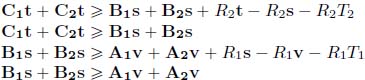
The equations then become, when we replace the service and arrival curves by their expression,
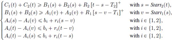
Note that the first two lines can be replaced by

We can also translate the monotony and the causality at dates v, s, t into the following inequalities (we only need to define ![]() at s and
at s and ![]() at t):
at t):
Let us denote by ![]() the arrival date of the bit of data of interest. We must have
the arrival date of the bit of data of interest. We must have ![]() (the bit of interest could arrive in a burst or, more specifically here, be the last bit of data of a burst).
(the bit of interest could arrive in a burst or, more specifically here, be the last bit of data of a burst).
In order to compute a bound for the worst-case delay of flow 2, it then suffices to solve those equations. It should be noted that if we accept replacing ![]()
![]() , all of the inequalities are linear and thus can be solved by a linear program. This linear program is given in Table 11.1. Here and in the rest of the chapter, we differentiate the variables from the quantity they represent (which can be a date or the value of a function at a date) by writing the variables in bold font and forgetting the parenthesis. For example, variable t is the variable representing date t and variable A1t is the variable representing
, all of the inequalities are linear and thus can be solved by a linear program. This linear program is given in Table 11.1. Here and in the rest of the chapter, we differentiate the variables from the quantity they represent (which can be a date or the value of a function at a date) by writing the variables in bold font and forgetting the parenthesis. For example, variable t is the variable representing date t and variable A1t is the variable representing ![]() .
.
Table 11.1. Linear program for computing the worst-case delay in a network of two servers in tandem
|
Objective |
Maximize t — v |
|
Under the constraints |
|
Dates |
|
|
Monotonicity |
|
|
Causality |
|
|
Arrival |
|
|
Service |
 |
In fact, this linear program gives the exact worst-case delay of the network, as we will prove in the following section.
11.1.2. A linear program for tandem networks
We first present the general scheme of transformation of a tandem network into a linear program before proving that its optimal solution is the exact worst-case delay of the network. Note that these results can be generalized at no cost to tree networks and adapted to the computation of the maximum backlog at a server.
Worst-case performance bounds can be computed using the linear program under the following assumptions on the arrival and service curves:
- – arrival curves are concave and piecewise linear (we can write
 );
); - – strict service curves are convex and piecewise linear (
 ).
).
We assume without loss of generality that flow 1 is the flow of interest and that this flow departs the network at server n.
11.1.2.1. Variables
There are two types of variables, namely time variables, which represent dates, and function variables, which represent the values of the functions at some of these dates:
- – time variables: th for all
 , as well as a variable u. Interpretation: tn represents the instant at which the worst case occurs: it is the departure time of the bit of data that suffers the maximal delay. Then,
  , the start of the backlogged period of th+1 at the server h. Variable u represents the arrival time u of the bit of data suffering the maximal delay in the first server;
 - – function variables (departure processes):
 and
and  for all
 . Interpretation: represents the value of the departure cumulative function of flow i at server h (or equivalently if flow i crosses server
  , the arrival cumulative function of flow i at server ) at times
  and
and  ;
; - – function variables (arrival processes):
 for all
  , and
, and  . Interpretation: represents the value of the cumulative function
  at time
  .
.
11.1.2.2. Linear constraints
The linear constraints can be intuitively deduced from the interpretation of the variables:
- – time constraints:
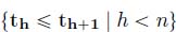 ;
; - – starts of backlogged periods:
 ;
; - – strict service constraints:

 (this inequality represents several linear inequalities, since
  is the maximum of linear functions);
 - – causality constraints:
 ;
;
- – non-decreasing functions:
 and
and  ;
; - – arrival constraints:

 (this inequality represents several linear inequalities, since
  is the minimum of linear functions);
 - – insertion of u:

 .
.
11.1.2.3. Objective
Depending on the worst-case performance to compute, two different objectives can be used:
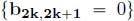
- – worst end-to-end delay for flow 1: maximize tn− u;
- – worst backlog at server n : maximize
 . Note that intuitively one should have
  instead of
  , but this variable is not defined in our linear program. In fact, the worst-case backlog at server n is obtained when all the other servers serve instantaneously their backlog, which corresponds to the objective. When computing the worst-case backlog, variable u and the related linear constraints can be dropped.
11.1.3. The equivalence theorem
THEOREM 11.1.– Let ![]() be a tandem network with n servers and m flows. Then, given a flow i (respectively a server j), the linear program described above has
be a tandem network with n servers and m flows. Then, given a flow i (respectively a server j), the linear program described above has ![]() variables and
variables and ![]() constraints and the optimum is the worst end-to-end delay for flow i (respectively the worst backlog at server j).
constraints and the optimum is the worst end-to-end delay for flow i (respectively the worst backlog at server j).
PROOF.– There are n + 2 time variables; the number of variable indices by flow i is linear in the length of its path, then in ![]() . Hence, the number of variables is in
. Hence, the number of variables is in ![]() . The number of constraints of each type is in
. The number of constraints of each type is in ![]() (this order is achieved for the arrival curve constraints).
(this order is achieved for the arrival curve constraints).
Let D be the optimal solution of the linear program for a tandem network.
There are two steps in the rest of the proof: first, we prove that for any admissible trajectory with maximum delay d, we can set variables satisfying all the constraints (hence d ≤ D), and the problem has value d; second, we prove that from a solution to the linear problem, we can reconstruct an admissible trajectory (hence d ≥ D).
First, consider an admissible trajectory and then set tn the departure time of the bit of data and u its arrival time. Set tn = tn; from the value assigned to tn and the interpretation of the variables, we can deduce the assignment of any other variable except those involving u. Set u = u and ![]() . As the trajectory is admissible and the constraints only encode network calculus constraints, it should be clear to the reader that every linear constraint is satisfied, and the delay of the bit of data is tn − u.
. As the trajectory is admissible and the constraints only encode network calculus constraints, it should be clear to the reader that every linear constraint is satisfied, and the delay of the bit of data is tn − u.
Second, consider a solution to the linear program:
- – the arrival cumulative process of flow i,
 , is defined by taking the largest non-decreasing function that is αi-constrained and takes values
  at time
  (note the special case for flow 1), and we only consider dates
  and u;
 - – the departure cumulative process
 is defined by having
 for all
  , for all
  and the linear interpolation
  otherwise.
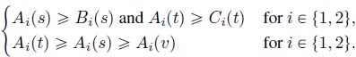
We now prove that the trajectory defined by these processes is admissible. By construction, these functions are non-decreasing, we have ![]() and the arrival processes are constrained by their arrival curves. Then, it remains to show that
and the arrival processes are constrained by their arrival curves. Then, it remains to show that ![]() is a strict service curve for server h. Let F be the aggregated departure process from server h. The strict service property has to be checked only on
is a strict service curve for server h. Let F be the aggregated departure process from server h. The strict service property has to be checked only on ![]() as it is the only backlogged period. In this interval, the processes are linear, so there exists H such that
as it is the only backlogged period. In this interval, the processes are linear, so there exists H such that ![]() . But as
. But as ![]() is convex and
is convex and ![]()
![]() , we have
, we have ![]() , hence the result.
, hence the result.
□
11.2. Tandem networks under the FIFO policy
In this section, we specialize the results with FIFO servers. Unfortunately, the linear program that we will obtain will not be solvable in polynomial time: the number of variables becomes exponential in the size of the network, and some of these variables are Boolean. However, this linear program will allow us to derive upper and lower bounds for the worst-case delay.
11.2.1. Single node
Let us first focus on the simple yet meaningful example of one server offering a min-plus service curve β crossed by two flows, whose respective arrival and departure processes are denoted by A1, A2 and D1, D2. For each departure date t1 of a bit, there exists another date t2 when that bit arrived. From Definition 7.7, if functions Ai are continuous at t2, then ![]() . Moreover, from Definition 5.3, (D1 + D2)(t1)
. Moreover, from Definition 5.3, (D1 + D2)(t1) ![]() β ∗ (A1 + A2)(t1). If β is convex, it is continuous, and then, there exists t3 such that D1(t1) + D2(t1)
β ∗ (A1 + A2)(t1). If β is convex, it is continuous, and then, there exists t3 such that D1(t1) + D2(t1) ![]() (A1(t3) + A2(t3)) + β(t1 − t3). As β
(A1(t3) + A2(t3)) + β(t1 − t3). As β ![]() 0, we can set t3
0, we can set t3 ![]() t2. Then, the worst-case delay, with a rate-latency service curves and token-buckets arrival curves, is computed by solving the problem of Table 11.2. We use the same convention as in the previous section, and bold letters represent variables of the linear program.
t2. Then, the worst-case delay, with a rate-latency service curves and token-buckets arrival curves, is computed by solving the problem of Table 11.2. We use the same convention as in the previous section, and bold letters represent variables of the linear program.
Table 11.2. Linear program for computing the worst-case delay in an FIFO server
|
Objective |
Maximize t1 − t2 |
|
Under the constraints |
|
Dates |
|
|
Monotonicity |
|
|
Arrival |
|
|
Service |
|
|
FIFO |
In Table 11.2, we use very simple curves, but these can be generalized to piecewise linear concave arrival curves and piecewise linear convex service curves by writing several arrival and service constraints.
11.2.2. Tandem networks
We now consider a tandem of n servers, with flow 1 as the flow of interest, traversing every server. Let us first focus on server n. Most of the constraints of Table 11.2 can be written down, generalized to the set of all flows crossing server n. However, arrival constraints cannot be formulated for flows starting before server n. Therefore, given a departure date at server n, t1 , we can compute two input dates, related to the FIFO and service curve constraints at server n, t2 and t3. Those dates also describe the output of server n − 1. Thus, we can iterate the previous reasoning at server n − 1, for each of the two dates: the bit that exits server n − 1 at time t2 entered that server at time t4, and t5 is a time instant in the past that verifies the service curve constraint formulated at time t2. Similarly, for date t3 at server n − 1, we can identify dates t6 and t7, respectively. It is easy to see that we can go backwards until server 1, doubling the number of dates and constraints at each node and adding arrival constraints whenever we hit the ingress node of a flow. In this way, we eventually set up a set of constraints that relate the dates of departure (at server n) and arrival of a bit of the tagged flow. Thus, we compute its worst-case delay by solving the linear problem that maximizes the above difference under these constraints.
More formally, the variables of our problem are the following:
- – time variables: t1,…,
 , where t2k and t2k+1 correspond to the FIFO and the service curve constraints with regard to tk;
 - – function values:
 for fst(i) — 1
  h
h  end(i) and k ∈ [2n+1−h 2n+2−h – 1].
The number of dates (hence of variables) grows exponentially with the tandem length, since it doubles at each node as we go backwards. Unfortunately, in a multi-server scenario, these dates are only partially ordered. Following the argument for the single server case and the network calculus constraints, we have:
- – (*) for k < 2n, t2k+1
 t2k
t2k  tk;
tk; - – (**) if 2h
 k,
k,  < 2h+1 and if tk
  , then t2k
  (cumulative functions are non-decreasing) and t2k+1
  (same as above, plus β( h) is convex).
These relations and the transitivity only lead to a partial order of ![]() . For example, for a two-node tandem, we have t1
. For example, for a two-node tandem, we have t1 ![]() t2
t2 ![]() t3, and t4
t3, and t4 ![]() t5, t4
t5, t4 ![]() t6, t5
t6, t5 ![]() t7 and t6
t7 and t6 ![]() t7. However, t5 and t6 cannot be ordered. A partial order creates a problem. Given a partial order of dates, we can enforce the same partial order on the corresponding function values, but this is not sufficient to ensure the monotonicity of the cumulative arrival and departure processes. In fact, it may well happen that, in the above example, the optimal solution to the linear program is for t5 < t6 and
t7. However, t5 and t6 cannot be ordered. A partial order creates a problem. Given a partial order of dates, we can enforce the same partial order on the corresponding function values, but this is not sufficient to ensure the monotonicity of the cumulative arrival and departure processes. In fact, it may well happen that, in the above example, the optimal solution to the linear program is for t5 < t6 and ![]() , for some i, h, which violates monotonicity. In this case, the solution does not correspond to any feasible scenario and hence it is not the worst-case delay. To ensure monotonicity in a linear programming approach, we need to introduce Boolean variables.
, for some i, h, which violates monotonicity. In this case, the solution does not correspond to any feasible scenario and hence it is not the worst-case delay. To ensure monotonicity in a linear programming approach, we need to introduce Boolean variables.
LEMMA 11.1.– Consider the following constraints:

Then, x1 < x2 ![]() y1
y1 ![]() y2 and x2 < x1
y2 and x2 < x1 ![]() y2
y2 ![]() y1.
y1.
PROOF.– The inequality x1 < x2 imposes that b = 0 and then that y2 ![]() y1. Similarly, x2 < x2 imposes that b = 1 and that y1
y1. Similarly, x2 < x2 imposes that b = 1 and that y1 ![]() y2.
y2.
□
This lemma can be used on all dates tk , ![]() on which cumulative processes are defined. Since a date corresponds to a unique node in the tandem, for a date tk, there exists a unique h such that
on which cumulative processes are defined. Since a date corresponds to a unique node in the tandem, for a date tk, there exists a unique h such that ![]() (tk) is defined; hence, it is sufficient to generate total orders on
(tk) is defined; hence, it is sufficient to generate total orders on ![]() for each h ∈ [1,n + 1].
for each h ∈ [1,n + 1].
Using the results of Chapter 10, the constant M is easy to find: it suffices to find an upper bound of the delay and of the cumulative arrival functions. We will not comment further on this value, but assume for every variable x the constraint 0 ![]() x
x ![]() M.
M.
We are now ready to define the constraints of a mixed-integer linear program (MILP) in order to compute the worst-case delay of flow 1. In the following, the expression ![]() stands for
stands for ![]() .
.
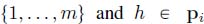
For all h ∈ {1,…,n + 1}, for all k, ![]() and for all i ∈ {1,…,m} such that h ∈ pi:
and for all i ∈ {1,…,m} such that h ∈ pi:
- – time constraints:
 ;
; - – partial order constraints:
 and
and  ;
; - – monotonicity:
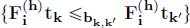 ;
; - – FIFO hypothesis: h >
 ;
; - – service constraint:
 ;
; - – arrival constraints: if h = fst(i),
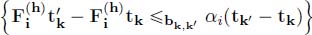 .
.
The objective of the linear program is then max t1 − ![]() .
.
THEOREM 11.2.– The worst-case delay for flow 1 is the optimal solution of the mixed-integer linear program just described.
PROOF.– Set d the worst-case delay for an admissible trajectory of the network and D the optimal solution of the MILP. The proof is in two steps: we first prove that every admissible trajectory is a solution of the MIPL, so that d ![]() D. Then, we show that from any solution of the MILP, we can construct an admissible trajectory, so that D
D. Then, we show that from any solution of the MILP, we can construct an admissible trajectory, so that D ![]() d.
d.
First, consider an admissible trajectory and set t1 the departure time of the bit of data of interest. Set t1 = t1. By definition, cumulative functions are left-continuous. Then, by Proposition 3.10, we can find a date t3 such that ![]() and a date t2 such that for all flow i crossing server n,
and a date t2 such that for all flow i crossing server n, ![]() . We can then set the variables as tk = tk and
. We can then set the variables as tk = tk and ![]() but for
but for ![]() .
.
By induction, we can go on assigning dates and variables ![]() if variables tk and
if variables tk and ![]() are assigned, we can assign
are assigned, we can assign ![]() and
and ![]() if
if ![]() the same way as with k = 1. Remark that
the same way as with k = 1. Remark that ![]() .
.
The reason why we cannot define t2k directly by ![]() is that the functions are not necessarily continuous. As a result, it may be the case that several dates defined have the same value, with different values for the functions. This is not a problem for mathematical programs. Also note that this assignment of variables also defines a total order of the dates, which allows us to assign variables
is that the functions are not necessarily continuous. As a result, it may be the case that several dates defined have the same value, with different values for the functions. This is not a problem for mathematical programs. Also note that this assignment of variables also defines a total order of the dates, which allows us to assign variables ![]() , so that the monotonic and arrival constraints are satisfied. As a result, the assignment of the variables respects all the constraints and they are a solution to the problem and
, so that the monotonic and arrival constraints are satisfied. As a result, the assignment of the variables respects all the constraints and they are a solution to the problem and ![]() .
.
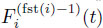
On the other hand, consider a solution of the MILP. We will define a scenario that verifies all the constraints. Assign dates ![]() for all k, fix i and h and consider the variables of the form
for all k, fix i and h and consider the variables of the form ![]() and tk for which
and tk for which ![]() is defined. Let
is defined. Let ![]()
![]() We set
We set ![]() and
and ![]() . If
. If ![]()
![]() , then from those values, we extrapolate
, then from those values, we extrapolate ![]() as the largest non-decreasing function that is
as the largest non-decreasing function that is ![]() -constrained and takes values
-constrained and takes values ![]() at time tk. If
at time tk. If ![]()
![]() , then we extrapolate
, then we extrapolate
We can check that:
- – those functions are wide-sense increasing (because of the Boolean variables);
- – arrival functions are α-constrained (by construction);
- – the FIFO order is preserved: it is preserved for the dates defined by the linear program, and outside of those dates, the traffic is only made up of bursts;
- – the service constraints are met by construction.
We have then built a scenario that verifies all the constraints and that has the same
delay as the solution of the linear program. Then, ![]() .
.
□
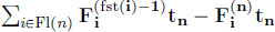
We remark that Theorem 11.2 can be generalized to compute the worst-case delay of any flow i by only modifying the objective function to maximize ![]() .
.
11.2.3. Bounds on the worst-case delay
As already pointed out, computing the worst-case delay in a tandem network requires an exponential number of (potentially Boolean) variables, which makes this solution intractable for large networks.
One solution to simplify the problem (which will remain exponential) is to relax some constraints, especially the Boolean ones. An upper bound can be found by giving up total ordering. We only keep the partial date and function value ordering and solve one linear program, forgetting all the Boolean variables.
Similarly, any solution of the MILP can be extrapolated into an admissible trajectory and hence is a lower bound on the worst-case delay. An algorithmically efficient way to obtain a lower bound is to reduce the number of dates, by imposing further constraints on the latter. We can do this by setting ![]() for
for ![]() . In this way, the number of different dates is quadratic in the number of nodes, and this induces a complete order on the dates for every h. Therefore, this lower bound can be obtained in polynomial time.
. In this way, the number of different dates is quadratic in the number of nodes, and this induces a complete order on the dates for every h. Therefore, this lower bound can be obtained in polynomial time.
11.3. Bibliographic notes
In this chapter, we have presented a few methods for computing exact worst-case performance bounds. To ease the presentation, we have restricted the approach to tandem networks. All of these methods can also be generalized to tree topologies with no algorithmic cost.
The linear programming approaches can also be generalized to general feed-forward networks for both the arbitrary multiplexing case [BOU 10b, BOU 16c] and the FIFO case [BOU 12b, BOU 16b], but the polynomial algorithms become exponential for two reasons. The first is that the number of constraints depends on the number of paths in the graph ending at server n, and there can be an exponential number of such paths. The second reason is the ordering of the time constraints. In the FIFO framework, the ordering is done the same way as presented in this chapter, i.e. by introducing Boolean variables, but in the arbitrary multiplexing approach, this trick is not possible because it is based on the backlogged periods, and an exponential number of linear programs have to be generated.
Adaptations of the linear program for the arbitrary multiplexing case can be used for other service policies, such as the static priorities in [BOU 11c]. It combines the modular approach to compute constraints on the arrival curves at every flow and every server and incorporate those curves as linear constraints in the linear program.
Other approaches have also been developed for computing worst-case performance bounds in a tandem network. In [BOU 15], a greedy algorithm is developed. It is based on a backward recursion from the last server to the first server, and computes for each flow the maximum amount of backlog that can be transmitted from one server to another. The proof strongly relies on a precise study of the properties of worst-case trajectories.