Introduction
With the emergence of a multitude of network architectures, performance evaluation, originating from Erlang’s work, has become an important research topic. The simplest model of a communication system is the queue, and by extension, these systems of queues have a high modeling power. A queue is composed of a waiting queue and a server that processes data in the waiting queue. If X (t) is the number of data in the queue at time t, C is the number of data that can be processed by unit of time and A(t) is the number of data entering the system between times t and t + 1, then the first (and most important) formula that can be written is the Lindley formula [LIN 52]:
Based on this formula, the queueing theory derives properties for X (t) based on the knowledge of C and A(t) given by some distributions and independence relations. Among the important results derived from this formula are the Pollaczek–Khinchine formula and the Little formula [LIT 61]. As far as stochastic models are concerned, queueing theory is still an active topic, and with the emergence of large and complex networks, new models have also been theory [BAC 02, LEB 07, GAS 12, DUF 10], stochastic geometry [BAC 09a, BAC 09b], random graphs [FRA 08, BOL 01, DRA 10] and so on.
Another direction of research is to make use of the “+” and the “max” in equation [I.1]. Then, systems of queues can be analyzed using the (max,plus) (or tropical) algebra [BAC 92]. Compared to classical algebra, the addition is replaced by the maximum, and the multiplication by the addition. In this type of system, the addition models the time evolution and the maximum models the synchronization of events. An alternative and dual model for such systems uses the (min,plus) algebras, which is the base of the network calculus theory, the topic of this book.
Unlike classical queueing theory, it is based on the study of envelopes and bounding processes rather than studying their exact value. Introduced by the seminal work of Cruz [CRU 91a, CRU 91b], in which the traffic is characterized by (σ, ρ)-envelopes to compute maximum delays, the notion of envelope has been formalized and generalized to functions with values in the (min,plus) dioid [CRU 95]. The elements of a network, namely wires, switches and processors, have also been generalized from conservative link (the amount of data that can be served during each unit of time is constant) to more general envelopes in the same functional space. The aim of this theory is to compute deterministic upper bounds of performances (such as transmission delay or buffer usage) in networks.
In this model, data flows and systems are abstracted by functions in the dioid of the (min,plus) functions and performances can be derived by combining those functions through (min,plus) operators, such as the (min,plus) convolution, the (min,plus) deconvolution or the sub-additive closure. The main references on the topic are the textbooks [CHA 00] and [LEB 01], and since the pioneer works of Cruz in the 1990s, thousands of papers on network calculus have been published and at least six academic and four industrial tools based on network calculus have been developed.
The target application was originally communication networks, such as the Internet. Network calculus was successfully applied to study networks with differentiated services (DiffServ), as it enables us to compute a guaranteed rate for the best effort flows and integrated services (IntServ), which guarantees a bandwidth for each flow [PAR 93, PAR 94, FID 04]. Another success is the application of network calculus to define efficient load-balanced switches, the Birkhoff–Von Neumann switch, for example, which has a periodic scheme to connect any input to any output during a time proportional to the bandwidth requested for this connection [CHA 01, CHA 02a, CHA 02b]. A third example of application in this field is video-on-demand (VoD) [MCM 06, DUF 98, GAN 11].
However, in other fields of communication networks, dimensioning the capacities of the network with regard to the worst-case performance leads to over-provisioning. Indeed, the transmission times are often not critical: worst-case performance is not the right parameter to study (it happens very rarely), whereas the mean or the variability of the transmission delay might be the parameters to study, as the users of the network might be more sensitive to a slower than usual network. As a result, stochastic models are more relevant. For this aim, the stochastic counterpart of network calculus has been developed, the stochastic network calculus [CHA 94, JIA 08, FID 15]. The aim of this theory is to compute the violation probability of some flow of data to have a certain maximum delay. Several models have been defined, but they all mix the network calculus theory with the deviation theory.
Another class of applications where deterministic network calculus is relevant is real-time and critical systems. These systems have hard deadlines and require a deterministic analysis. The most famous success of network calculus is certainly its use to bound the delay and the buffer usage of the AFDX (Avionics Full Duplex) network of the Airbus A380 airplane [FRA 06, BOY 08, BOY 10c], and recent developments of network calculus have been obtained in this context. AFDX is an embedded network based on the Ethernet technology, and is where switches are connected using full-duplex links, i.e. there are two different wires between two switches, one for each direction, avoiding collisions. A realistic network is composed of a dozen switches and thousands of flows, called virtual links. As a result, the techniques developed to analyze such networks must be algorithmically efficient and compute accurate upper bounds on the transmission delays.
In the field of embedded networks, network calculus competes with other techniques. Among them, we can cite model checking [CLA 99]. Model checking is based on the exhaustive modeling of the states of the system with objects such as timed automata (or recently adapted to the context of network calculus, event-count automata [CHA 05]) and computes the exact bounds by analyzing them. As a result, it will give very accurate bounds, but at a prohibitive algorithmic cost. For example, in [PHA 07], a three-node network can be analyzed in 30 minutes. A second and classical technique is scheduling. In the context of the AFDX network, the trajectorial approach has been developed [MAR 06]. Given a sporadic flow (almost periodic with jitters) and a packet of this flow, the aim is to find a bound on the worst-case delay suffered by this packet given the interacting flows. The equation that gives this worst-case delay can then be solved using a fix-point equation. These techniques have been designed to be more accurate than the network calculus. Unfortunately, flaws have been found in this theory, invalidating the results of first investigations [KEM 13b, KEM 13a], and although these have been corrected [LI 14], no comparison with network calculus has been done since this correction.
In this book, we propose to present what are in our opinion the most important results obtained in the deterministic network calculus theory, since its first developments. Indeed, no general book on the topic has been published since the publication of two reference books in the early 2000s.
I.1. Organization of the book
This book is composed of three parts: the first presents the mathematical framework of the network calculus theory, the second focuses on the analysis of a network element in isolation and the third shows how to analyze a whole network.
These three parts are preceded by Chapter 1, which introduces the model and explains our assumptions in the rest of the book. We take the example of a single server crossed by a single flow and show how the (min,plus) operators naturally appear in our model and how performances (delay and backlog) are computed.
The first part is about the mathematical framework, i.e. the dioid of (min,plus) functions:
- – Chapter 2 defines this dioid and all the (min,plus) operators that will appear, namely the convolution, deconvolution and sub-additive closure. In this chapter, we use an algebraic approach whenever possible, to stress the importance of the dioid structure of the theory;
- – Chapter 3 focuses on the classes of functions that are generally used for network calculus: functions are non-decreasing and important classes of functions are the convex and the sub-additive functions;
- – Chapter 4 deals with the algorithmic aspects of the (min,plus) functions. Indeed, the implementation of the (min,plus) operators is important in order to build network calculus tools. We present general procedures to compute the (min,plus) operators and also some efficient algorithms when restricting to some classes of functions. We also present containers that enable us to efficiently perform the operations on approximate functions.
The second part defines the network calculus model of a server and is devoted to the local analysis of networks:
- – Chapter 5 presents the foundations of the network calculus model, with the definitions of the arrival and service curves, that respectively model the data flows and the network elements. We show how performance bounds are computed from these curves;
- – Chapter 6 extends the model to the case of a flow crossing a sequence of servers. The pay burst only once phenomenon, demonstrating the importance of studying a network in its globality, is explored. Several important use cases are presented, including the flow-window control;
- – Chapter 7 presents the case of a network element crossed by several data flows. Here, the notion of residual service curve is introduced, allowing us to compute a service guarantee for every flow crossing the server. The residual service curve depends on the service policy of the server, and we study several of them;
- – Chapter 8 extends Chapter 7 by considering packets instead of fluid data, showing the modeling power of network calculus;
- – Chapter 9 ends the second part and offers a detailed comparison of the different notions of service curves that have been defined, including the real-time calculus theory.
The third part considers a whole network:
- – Chapter 10 presents different solutions to compute end-to-end delay bounds in feed-forward networks. The pay multiplexing only once phenomenon is exhibited, which emphasizes the difficulty of computing accurate performance bounds in networks;
- – Chapter 11 presents a completely different way to compute performance bounds in feed-forward networks, using linear programming. This method is less general, but when it applies, it allows us to compute tight performance bounds;
- – Chapter 12 closes this third part by considering a network with cyclic dependencies. Sufficient conditions for the stability are computed, depending on the topology (with the fix-point method) or the service policy.
I.2. How to read this book
While writing this book, we had the following concerns in mind:
1) self-satisfaction: we tried to be as comprehensive as possible from the modeling with the (min,plus) algebra to the more elaborate results. We provide proofs for all of the results presented, although some have been simplified to keep them compact;
2) rigor: we paid attention to technical details such as function domains and continuity, while also justifying the modeling choices. Indeed, our personal experience is that most errors in formal methods come either from such details or from a modeling that does not capture the reality of the systems;
3) audience diversity: every reader has different expectations when opening a technical book. We tried to take into account this variety by presenting different aspects of network calculus: an engineer might be mainly interested in the modeling power and the applicability of the theory, but a developer might be more interested in its algorithmic aspects and in the tools that have been developed. Finally, some researchers might want to delve deeper into the theoretical aspects.
Figure I.1 represents the interdependence of the chapters.
A reader focusing on the application of network calculus could almost skip Part 1: they can refer to the definitions of the (min,plus) operators and classes of function in the summaries of Chapters 2 and 3 for the notations. Therefore, from Chapter 1 which motivates the model, they can jump to Chapters 5 to 8 and then to Chapter 10 and eventually to Chapter 12, depending on the type of networks they want to analyze. Finally, they might be interested in the list of existing tools in the Conclusion.
The reader interested in the implementation of network calculus will also be interested in the first part of the book, which deals with the operators and their properties, and especially in Chapter 4.
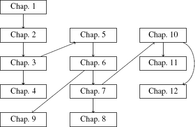
Figure I.1. Dependence between chapters
Some sections of this book are only of theoretical interest. This is particularly the case for Chapter 9, which compares the different types of service curves defined in the literature, and section 10.5, which proves the NP-hardness of computing tight performance bounds.
Finally, we shall use “WARNING.–” notes to emphasize counter-intuitive results.
I.3. Network calculus in four pages
In this section, we briefly present the model and the theory of network calculus. For readability, we do not mention the hypothesis required for the computations. The reader is referred to the rest of this book for more details.
Flow model: a flow of data crossing a given point of the network (from the input to the output of a server element) is described by a cumulative function A: A(t) is the amount of data crossing that point up to time t.
Server model: a network element (or server), represented in Figure I.2, is a relation between two cumulative functions: A, the arrival cumulative function (at the input of the server) and D, the departure cumulative function (at the output of the server). For modeling purposes, this relation is usually not a function.
Performance bounds: From A and D, the arrival and departure cumulative functions, respectively, and provided that data exit in the same order as they arrive, the maximum delay d(A, D) is the maximum horizontal distance between A and D, as illustrated in Figure I.3.
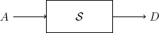
Figure I.2. Server: a relation between arrival and departure cumulative functions
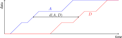
Figure I.3. Delay from the cumulative functions. For a color version of this figure, see www.iste.co.uk/bouillard/calculus.zip
An abstraction by curves: the exact behavior of a system is unknown at the design stage or too complex to be handled. The principle of network calculus is to abstract the flow and server by contracts, called arrival curves and service curves, respectively.
For the flows, the arrival curve bounds the amount of data during any interval of time: α is an arrival curve for A if
which translates into “the amount of data that arrived between time t and t + s is less than α(s)” and is illustrated in Figure I.4.
Symmetrically, a guarantee on the server is to bound the minimum amount of data that can be processed during any interval of time by the server. If β(s) is the minimum amount of data that the server can process in any time interval of length s, then β is a service curve. Of course, as the server can be empty and thus serve no data, D(t + s) — D(t) will not be lower-bounded by β(s). However, we can show that D can be expressed as a function of A and β.
Algebraic relations: the (min,plus) convolution * (defined in Chapter 2) enables us to relate the cumulative processes with the arrival and service curves:
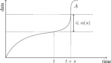
Figure I.4. Arrival curve of a flow
Performances from curves: from this modeling, it is now possible to compute bounds from the curves only. The maximum delay is bounded by the horizontal distance between α and β, and the maximum backlog (or buffer occupancy) by the vertical distance of the curves. Moreover, α ![]() β is an arrival curve for D, where
β is an arrival curve for D, where ![]() is the (min,plus) deconvolution which will be defined in Chapter 2.
is the (min,plus) deconvolution which will be defined in Chapter 2.
From this modeling, we now illustrate how these basic elements can be used to analyze more complex networks.
Sequence of servers: suppose that the flow of data crosses several servers as in Figure I.5. Due to the nice algebraic properties of the (min,plus) convolution, we can write ![]() which means that the sequence of servers S1 and S2 can be modeled as a server with service curve β1 * β2.
which means that the sequence of servers S1 and S2 can be modeled as a server with service curve β1 * β2.

Figure I.5. A single flow crossing two servers in tandem
The end-to-end delay can then be computed by d(α, β1 * β2). Another solution would be to add the maximum delay of each server: d(α, β1) + d(α![]() β1, β2).
β1, β2).
The pay burst only once phenomenon, a key result of network calculus detailed in Chapter 6, is the observation that
Residual service curves: suppose now that the server is crossed by several flows. The service curve represents the global guarantee for the server that is shared among the flows. Our goal is to compute residual service curves, i.e. service guarantees for each flow. These service guarantees will of course depend on the service policy of the server (FIFO, priorities, processor sharing, etc.), and on the characteristics of the other flows.

Figure I.6. Residual service curves
For example, when a server of capacity β is shared by two flows with respective arrival functions A1, A2 and arrival curves α1, α2, as in Figure I.6, the simplest result valid for any service policy is that a residual service offered to flow i is
where {i, j} = {1, 2} and ![]() will be defined in Chapter 3. This result seems quite simple and coherent with the intuition (each flow gets the minimal service minus the maximal interference), but technical assumptions have been omitted here and must be verified in Chapter 7.
will be defined in Chapter 3. This result seems quite simple and coherent with the intuition (each flow gets the minimal service minus the maximal interference), but technical assumptions have been omitted here and must be verified in Chapter 7.
Analysis of a network: let us now consider a more generic case as illustrated in Figure I.7.

Figure I.7. Topology with several flows crossing several servers
To analyze such generic topologies, the most common approach, called modular analysis, consists of mixing results on the sequence of servers and residual service curves.
In Figure I.7, an end-to-end service curve for flow 1 (described by the cumulative functions A1, B1 and C1) can be computed by
The case of flow 2 is a little more complicated as we also need to compute the residual service curve at server 4. This residual service curve can be computed by grouping flows 3 and 4: the end-to-end residual service curve for flow 2 is then:
The case of flows 3 and 4 can be handled differently: the same process would be possible, but in many cases, it is possible to group servers 3 and 4 first: denote ![]()
![]() the residual service curve for flows 3 and 4 at server 4. Then, the residual service curve for flow 3 can be computed as
the residual service curve for flows 3 and 4 at server 4. Then, the residual service curve for flow 3 can be computed as
and similarly for flow 4. This illustrates the pay multiplexing only once phenomenon: the interference with flow 3 counted only once. The different modular approaches will be detailed in Chapter 10.
Another approach, explained in Chapter 11, consists of writing the equations on cumulative functions for the whole network and considering the arrival and service curves as constraints on the system. The computation of the delay then boils down to an optimization problem.