
Chapter 2. PDF Imaging Model
In this chapter you’ll begin your exploration into the PDF imaging model—that is, the various types of graphic operations that can be carried out on the pages of a document. You’ll learn not only the language used to describe those operations, but also about various graphic and imaging concepts that accompany it.
Content Streams
As described in the previous chapter, a PDF file is composed of one or more pages (of a fixed size), and the visible elements on each page come from either the page content or a series of annotations that sit on top (visibly) of the content. This chapter discusses the page content.
Page content is described using a special text-based syntax (related to, but different from the PDF file syntax that you learned about in Chapter 1) that is stored in the PDF inside of a special type of stream object called a content stream. The content syntax is derived from Adobe’s Postscript language and is comprised of a series of operators and their operands, where each operand can be expressed as a standard PDF object (see PDF Objects). A simple example, for drawing a rectangle filled with the color blue, is given in Example 2-1.

We’ll look at the various operators themselves shortly, but for now, the most important thing to take away from the example is that the syntax is expressed in Reverse Polish Notation, where the operator follows the operands (if any). The second thing you should remember about the page syntax language is that, unlike Postscript, it’s not a true programming language in that it has no variables, loops, or conditional branching.
The content operators can be logically broken down into three categories. The most important ones, of course, are the drawing operators that cause something to be actually drawn onto the page. However, the drawing operators wouldn’t be fully useful without the ability to set the attributes of the graphic state that defines how the drawing will look (such as the color or pen width). Finally, there are a set of operators called marked content operators that let you apply special properties to a group of operators.
Graphic State
As mentioned, drawing wouldn’t be useful if you couldn’t set all the attributes of the drawing. Thus, we’ll start with the graphic state and its operators. You can think of the graphic state as a class or structure with members or properties and associated setters for changing the values. There are no getters, since there are no variables or conditionals in the content syntax to assign the values to or perform any operations on. This is extremely important, since it means that there isn’t a direct means to change some values in the graphic state and then set them back to what they were previously. You might think this means you either need to draw all “like objects” together or do a lot of “resetting.” Fortunately, you don’t have to do either! A PDF processor is required to maintain a stack (in the traditional programming sense) of graphic state, that the content stream can push new states onto or pop completed states off of. This way, you can save the state, do something, then return to the previous state. The operators for doing this are q and Q (see Example 2-2).
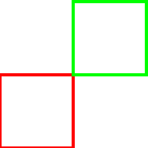
4 w                    % set the line width to 4, for all objects
q                      % push/save the state
1 0 0 RG               % set the stroking color to red
0 0 100 100 re         % draw a rectangle 100x100 with bottom left at 0,0
S                      % stroke with a 4-unit width
Q                      % pop the state
q                      % push/save the state
0 1 0 RG               % set the stroking color to green
100 100 100 100 re     % draw a rectangle 100x100 with bottom left at 100,100
S                      % stroke with a 4-unit width
Q                      % pop the state
In this example, we used an operator that you hadn’t seen before (w) to set the width of the pen in the graphic state. As you might imagine, this is a common operation.
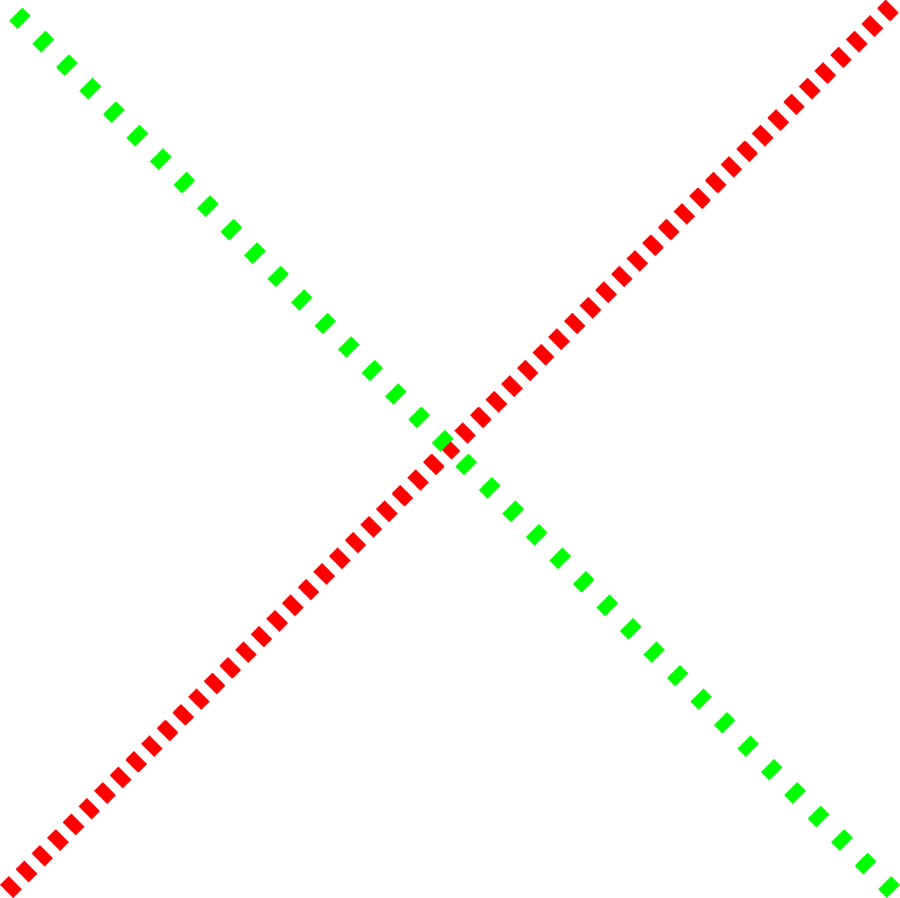
Additionally, there are a few other types of attributes that you can set when working with lines (or stroking of any shape), including dash patterns and what happens when two lines connect or join. Example 2-3 is an example of drawing two dashed lines.
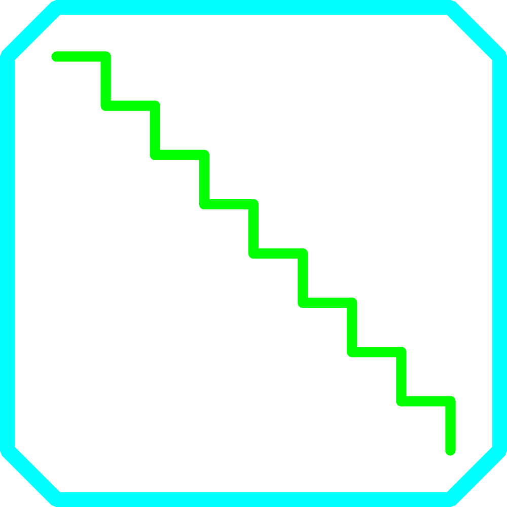
Example 2-4 shows the different types of line joins and caps (ends of a line).
          q
          0 1 0 RG
          10 w
          1 j                    % set the line join to round
          1 J                    % set the line cap to round
          100 500 m
          150 500 l
          150 450 l
          200 450 l
          200 400 l
          250 400 l
          250 350 l
          300 350 l
          300 300 l
          350 300 l
          350 250 l
          400 250 l
          400 200 l
          450 200 l
          450 150 l
          500 150 l
          500 100 l
          S
     Q
     q
          0 1 1 RG
          15 w
          2 j                    % set the line join to bevel
          50 500 m
          100 550 l
          500 550 l
          550 500 l
          550 100 l
          500 50 l
          100 50 l
          50 100 l
          h                      % makes sure that the shape is a closed shape
          S
     Q
The Painter’s Model
If you look at the previous examples, you’ll see that the way you draw shapes (or paths, as they are called in PDF terms) is to first define or construct the path and then either stroke (S), fill, (F/f), or both (B) the path. Each path is drawn in the order that it appears in the content stream, in a form of “first in, first out” (FIFO) operation. What that means is that if you want to draw one path on top of another, you just draw it after. The combination of these two attributes is usually called the Painter’s Model.
Note
The Painter’s Model is also used by graphic systems such as SVG and Apple’s Quartz 2D.
Example 2-5 illustrates how this works.
Open versus Closed Paths
Another aspect of the model is that shapes can be open or closed, which determines how the various stroking and filling operations complete when they reach the end of a path. Consider a path like the one in Example 2-6 that consists of a move to point A, then a line to point B, and another line to point C.
If you were to use the S operator that you’ve seen in our examples so far, that would draw an L-shaped line, since it simply strokes the path as defined. However, if you used the s operator, you would instead have a triangle, since the path would be closed (i.e., connected from the last point back to the first point) and then stroked. You can explicitly close a path using the h operator as well, and then use S to stroke it—so you can therefore consider s as a nice shorthand.
Clipping
The final aspect of the model that we’ll explore here is that of clipping. Clipping uses a path (or text) to restrict the drawing area from the full page to an arbitrary area on that page. This is most useful when you wish to show only a small portion of some other object (usually, but not necessarily limited to, raster graphics) for a specific visual effect.
Use the W operator to mark the path as a clipping path. You can then either continue to fill or stroke it (using the operators you’ve already seen), or do no drawing with the n operator.
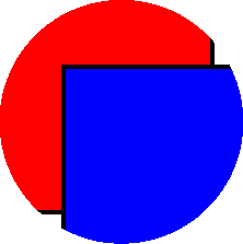
q
    27.738 78.358 m
    27.738 56.318 45.604 38.452 67.643 38.452 c
    67.643 38.452 l
    89.681 38.452 107.548 56.318 107.548 78.358 c
    107.548 78.358 l
    107.548 100.396 89.681 118.262 67.643 118.262 c
    67.643 118.262 l
    45.604 118.262 27.738 100.396 27.738 78.358 c
    W n                % clip with no actual drawing
    1 0 0 rg
    0 0 0 RG
    97.5 48.5 -98 97 re
    B
    0 0 1 rg
    146.5 -0.5 -98 97 re
    B
Q
Drawing Paths
While you could certainly do a lot of drawing with the three path construction operators you’ve seen so far (m, l, and re), you could do even more if you could draw something that wasn’t straight—say a curve, for example.
The c operator allows you to draw a type of curve called a Bézier curve (Figure 2-1), and specifically a cubic Bézier. Such a curve is defined from the current point to a destination point, using two other points (known as control points) to define the shape of the curve. It requires a total of six operands.
![“Example Bézier curve"][float="true”](http://imgdetail.ebookreading.net/data/56/9781449327903/9781449327903__developing-with-pdf__9781449327903__httpatomoreillycomsourceoreillyimages1821123.png)
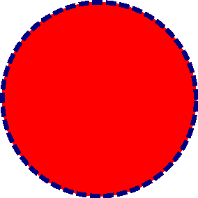
While Bézier curves are extremely flexible and enable very complex drawings, they do have a fundamental flaw: they cannot be used to draw a perfect circle. The closest you can get is to combine four curves that start and end at the four edge points on the circle, using a control point about 0.6 units from the end points.
Note
If you’d like to learn more about the mathematics for determining arcs and circles, the details can be found online.
Example 2-8 draws a circle, and also demonstrates how a path can be both stroked and filled using different colors.
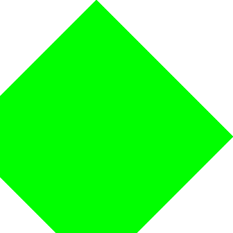
Transformations
As discussed in the first chapter, each page (see Pages) defines an area (in user units) into which you can place content. Normally, the origin (0,0) of the page is at the bottom left of the page, with the y value increasing up the page and the x value increasing to the right. This is consistent with a standard Cartesian coordinate system’s top-right portion. However, for certain types of drawing operations you may want to adjust (or transform, which is the proper term) the coordinates in some way—inverting/flipping, rotating, scaling, etc (see Figure 2-2).
The part of the graphic state that tracks this is called the current transformation matrix (CTM). To apply a transformation, you use the cm operator, which takes six operands that represent a standard 3x2 matrix. The chart below shows the most common types of transformations and which operands are used for them.
Transformation |
|
Translation |
|
Scaling |
|
Rotation |
|
Skew |
|
![“Picture of the four types of transformations"][float="true”](http://imgdetail.ebookreading.net/data/56/9781449327903/9781449327903__developing-with-pdf__9781449327903__httpatomoreillycomsourceoreillyimages1821125.png)
Example 2-9 gives a few examples of common transformations.
In some cases you will need to do multiple transformations, an operation called concatenating the matrix. The most common operation that requires concatenation is rotation (see Example 2-10). Not only is it more complex than other types of transformation since it involves the use of trigonometry, but it involves multiple operations. The reason for this in many cases is that rotation is always done around the bottom left of the object and not the center, which most people expect. Therefore, in order to handle rotation around the center point (or any arbitrary point), you need to first do a translation, and then a rotation, then transform back.
Basic Color
In the examples so far, we’ve always used RGB-based colors (called DeviceRGB in PDF terms). That’s the most common type of color that users are familiar with, since it’s what computer monitors use. In each example, we’ve used either a 1 or a 0 for each individual color component value. Unlike in other RGB color systems, such as Windows GDI or HTML, in PDF the value for each component is a real number between 0 and 1 rather than an integer value between 0 and 255.
Note
If you need to convert, the math is quite simple: pdfValue = 255 – gdiValue/255.
PDF, however, supports ten other color spaces (or color models) that can be used to specify the color of an object. This section introduces the two other Device color spaces: DeviceGray and DeviceCMYK. To learn more about the other eight color spaces as well as how to use patterns or shading to stroke or fill an object, see ISO 32000-1:2008.
For colors that use only shades of black and white (or gray), you can use the simple DeviceGray color space. The operators are g (for fill) and G (for stroke), and they take a single operand ranging from 0 (black) to 1 (white). This color space should be used instead of RGB-based black whenever possible as it produces higher quality printing operations while saving space in the PDF (3 bytes per operation vs. 8 bytes per operation).
While screens use RGB to define colors, printers use a different model called CMYK, for the Cyan, Magenta, Yellow, and blacK ink cartridges that are present in the printer. Higher-end printers may also have various other color inks, but they are used in other ways. To describe a color in DeviceCMYK, you use the k or K operators along with four operands for each of the color components.
Example 2-11 illustrates the use of the three color spaces.

Marked Content Operators
In Content Streams, it was mentioned that there were a set of operators whose job was to simply mark a section of content for a specific purpose. These operators are called “marked content operators,” and there are five of them, grouped into two categories. The MP and DP operators designate a single point in the content stream that is marked, while the BMC, BDC, and EMC operators bracket a sequence of content elements within the content stream.
Note
As stated, the marking must be around complete content elements and not simply a string of arbitrary bytes in the PDF. Additionally, the marked section must be contained within a single content stream.
To mark a single point in the content, perhaps to enable it to be easily located by a custom PDF processor, the MP or DP operator is used in conjunction with an operand of type Name, sometimes called a “tag.” The difference between MP and DP is that the DP operator also takes a second operand, which is a property list (see Property Lists). Example 2-12 shows a few examples.
% a content stream somewhere in a PDF
% we are using ABCD_ as an arbitrary second class name
/ABCD_MyLine    MP
q
    10 10 m
    20 20 l
    S
Q

/ABCD_MyLineWithProps << /ABCD_Prop (Red Line) >> DP
q
    1 0 0 RG
    10 200 m
    100 200 l
    S
Q
In the same way, the BMC and BDC operators, respectively, take either just a single tag operand or the tag plus a property list. These operators, however, start a section of marked content whose end is defined by the EMC operator. As you can see in Example 2-13, these operators are more useful than the simple point versions as they actually delineate the operators that are part of the group.
% a content stream somewhere in a PDF
% we are using ABCD_ as an arbitrary second class name
/ABCD_MyLine    BMC
    q
        10 10 m
        20 20 l
        S
    Q
EMC

/ABCD_MyLineWithProps << /ABCD_Prop (Red Line) >> BDC
    q
        1 0 0 RG
        10 200 m
        100 200 l
        S
    Q
EMC
Property Lists
When using the marked content operators DP and BDC, a dictionary is associated with the content as well. This dictionary is referred to as a property list and contains either information specific to the use of the content (such as with optional content) or private information meaningful to the writer creating the marked content (or a custom processor of the PDF).
Simple property lists, where all the values of all the keys are direct objects, may be written inline in the content stream as direct objects (as seen in the previous example). However, should any of the values of any of the keys require indirect references to objects outside the content stream, the property list dictionary needs to be defined as a named resource in the Properties subdictionary of the current resource dictionary and then referenced by name.
Resources
For content consisting only of paths in simple color spaces, the content stream is completely self-contained and needs no external references to other things. However, for most real-world PDF pages you will need other types of content, such as bitmap/raster images and text. These external references are managed via the resource dictionary that is the value of the Resources key in the page dictionary (see Example 2-14). Each key in the resource dictionary has a predefined name, based on the type of resource that is being listed. And the value of each key is itself a dictionary with the unique (and arbitrary) name for each resource and the indirect reference to the resource. It is common practice to use (short) identifying names/prefixes (such as GS for graphic state, IM for image, etc.) and then incrementally number as you go along. However, if you’d like to name them Manny, Moe, and Jack—that’s fine too!
% in the page dictionary
/Resources <<
    /Font <<
        /F1 10 0 obj
        /F2 11 0 obj
    >>
    /XObject <<
        /Im1 12 0 obj
    >>
>>
Don’t worry too much about the details of resources yet; you’ll be looking at them in specific examples as you continue.
External Graphic State
In all the examples we’ve looked at so far, all of the graphic state attributes have been applied directly in the content stream. This is mostly because we are using them only once, plus they happen to be simple attributes. However, there will be times when you’ll want to keep something like a “predefined style” and simply reference it by name. Like stylesheets in other formats (such as HTML or DOCX), this allows for easy updating of the style without impacting the content (stream), while also keeping file size down and performance up. In PDF, these styles are invoked using something called a graphic state parameter dictionary, or ExtGState (short for External Graphic State, so called because they are external to the content stream).
To use one, you add the dictionary to the page dicitonary’s resource dictionary (as an entry in the ExtGState dictionary, of course) and then use the gs operator in the content stream to invoke it. For example, to define a graphic state that uses a customized dash pattern at a large width, you could do the following (see Example 2-15):
% in the page dictionary
/Resources <<
    /ExtGState <<
        /GS0 <<
            /Type /ExtGState
            /LW 10                   % 10 wide
            /LC 1                    % rounded caps
            /D [[2 4 6 4 2] 2]       % dash pattern
        >>
    >>
>>

% in the content stream
/GS0 gs
0 1 0 0 K
100 100 m
100 400 l
S
Now that you’ve seen how to use ExtGStates as an alternative to inlining various attributes, let’s look at something that can’t be done inline, but only by using an ExtGState.
Basic Transparency
The PDF graphics model supports an extremely rich set of features in the area of transparency, which you can explore in detail in ISO 32000-1:2008, clause 11. For now, however, we’ll look at some basic transparency that is similar to what you might be used to with other imaging models (such as GDI+).
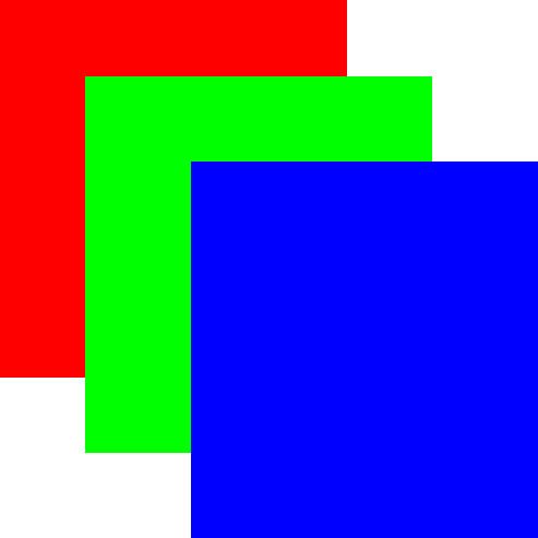
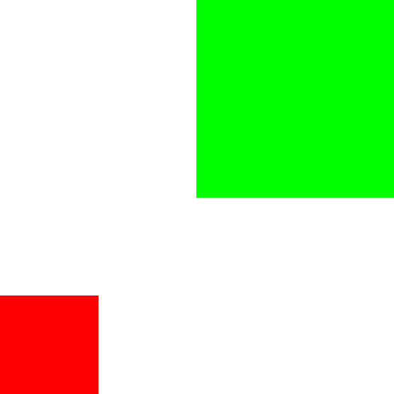
The simplest type of transparency is applying a level or percentage (as a number from 0 to 1) to how transparent (or opaque) a given object is. An object with a transparency value of 0 is completely invisible, while a value of 1 (the default) is completely opaque. Any value in between means that whatever is underneath will show through (or, to use the technical term, will “blend” with the transparent object), to a greater or lesser extent. As with other graphic state attributes, you can set the stroke and fill transparency values separately using the CA and ca keys, respectively, in an ExtGState dictionary.
The reason that transparency is handled as part of the ExtGState dictionary instead of directly in the content stream was to provide compatibility with older readers at the time it was introduced into PDF (version 1.4). Example 2-16 gives a few exmaples of transparency.

% in the page dictionary
/Resources <<
    /ExtGState <<
        /GS0 <<
            /CA 1
            /ca 1
        >>
        /GS1 <<
            /CA .5
            /ca .5
        >>
        /GS2 <<
            /CA .75
            /ca .75
        >>
    >>
>>

% in the content stream
q
    /GS0 gs    % no transparency
    1 0 0 rg
    209 426 -114 124 re
    f
Q
q
    /GS1 gs    % .5 transparency
    0 1 0 rg
    237 401 -114 124 re
    f
Q
q
    /GS2 gs    % .75 transparency
    0 0 1 rg
    272 373 -114 124 re
    f
Q
What’s Next
In this chapter, you learned about content streams and many of the things that can be found inside them. You also learned about how to reference external things via named resources. However, so far we’ve only covered how to draw vector graphics (paths), not any of the other types of content that PDF supports—most especially, text and images.
Next we’ll look at images, focusing on raster but also some additional ways to work with vector graphics. Following that, we’ll tackle text.