
Chapter 1
Signals and Spectra
This book presents the ideas and techniques fundamental to digital communication systems. Emphasis is placed on system design goals and on the need for trade-offs among basic system parameters such as signal-to-noise ratio (SNR), probability of error, and bandwidth expenditure. We shall deal with the transmission of information (voice, video, or data) over a path (channel) that may consist of wires, waveguides, or space.
Digital communication systems are attractive because of the ever-growing demand for data communication and because digital transmission offers data processing options and flexibilities not available with analog transmission. In this book, a digital system is often treated in the context of a satellite communications link. Sometimes the treatment is in the context of a mobile radio system, in which case signal transmission typically suffers from a phenomenon called fading, or multipath. In general, the task of characterizing and mitigating the degradation effects of a fading channel is more challenging than performing similar tasks for a nonfading channel.
The principal feature of a digital communication system (DCS) is that during a finite interval of time, it sends a waveform from a finite set of possible waveforms; in contrast, an analog communication system sends a waveform from an infinite variety of waveform shapes with theoretically infinite resolution. In a DCS, the objective at the receiver is not to reproduce a transmitted waveform with precision; instead, the objective is to determine from a noise-perturbed signal which waveform from the finite set of waveforms was sent by the transmitter. An important measure of system performance in a DCS is the probability of error (PE).
1.1 Digital Communication Signal Processing
1.1.1 Why Digital?
Why have communication systems, military and commercial alike, “gone digital”? There are many reasons. The primary advantage is the ease with which digital signals, compared with analog signals, are regenerated. Figure 1.1 illustrates an ideal binary digital pulse propagating along a transmission line. The shape of the waveform is affected by two basic mechanisms: (1) As all transmission lines and circuits have some nonideal frequency transfer function, there is a distorting effect on the ideal pulse; and (2) unwanted electrical noise or other interference further distorts the pulse waveform. Both of these mechanisms cause the pulse shape to degrade as a function of line length, as shown in Figure 1.1. During the time that the transmitted pulse can still be reliably identified (before it is degraded to an ambiguous state), the pulse is amplified by a digital amplifier that recovers its original ideal shape. The pulse is thus “reborn,” or regenerated. Circuits that perform this function at regular intervals along a transmission system are called regenerative repeaters.
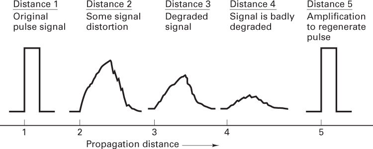
Figure 1.1 Pulse degradation and regeneration.
Digital circuits are less subject to distortion and interference than are analog circuits. Because binary digital circuits operate in one of two states–fully on or fully off–to be meaningful, a disturbance must be large enough to change the circuit operating point from one state to the other. Such two-state operation facilitates signal regeneration and thus prevents noise and other disturbances from accumulating in transmission. Analog signals, however, are not two-state signals; they can take an infinite variety of shapes. With analog circuits, even a small disturbance can render the reproduced waveform unacceptably distorted. Once the analog signal is distorted, the distortion cannot be removed by amplification. Because accumulated noise is irrevocably bound to analog signals, these signals cannot be perfectly regenerated. With digital techniques, extremely low error rates producing high signal fidelity are possible through error detection and correction, but similar procedures are not available with analog.
There are other important advantages to digital communications. Digital circuits are more reliable and can be produced at a lower cost than analog circuits. Also, digital hardware lends itself to more flexible implementation than analog hardware [e.g., microprocessors, digital switching, and large-scale integrated (LSI) circuits]. The combining of digital signals using time-division multiplexing (TDM) is simpler than the combining of analog signals using frequency-division multiplexing (FDM). Different types of digital signals (data, telegraph, telephone, television) can be treated as identical signals in transmission and switching: A bit is a bit. Also, for convenient switching, digital messages can be handled in autonomous groups called packets. Digital techniques lend themselves naturally to signal processing functions that protect against interference and jamming or that provide encryption and privacy. Also, much data communication is from computer to computer, or from digital instruments or terminal to computer. Such digital terminations are naturally best served by digital communication links.
Some costs are associated with the beneficial attributes of digital communication systems. Digital systems tend to be very signal processing intensive compared with analog. Also, digital systems need to allocate a significant share of their resources to the task of synchronization at various levels. (See Chapter 10.) With analog systems, on the other hand, synchronization often is accomplished more easily. One disadvantage of a digital communication system is nongraceful degradation. When the signal-to-noise ratio drops below a certain threshold, the quality of service can change suddenly from very good to very poor. In contrast, most analog communication systems degrade more gracefully.
1.1.2 Typical Block Diagram and Transformations
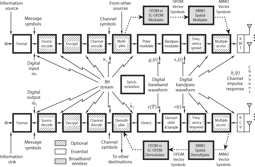
The functional block diagram shown in Figure 1.2 illustrates the signal flow and the signal processing steps through a typical DCS. This figure can serve as a kind of road map, guiding the reader through the chapters of this book. The upper blocks denote signal transformations from the source to the transmitter (XMT). The lower blocks denote signal transformations from the receiver (RCV) to the sink, essentially reversing the signal processing steps performed by the upper blocks. The modulate and demodulate/detect blocks together are called a modem. The term modem often encompasses several of the signal processing steps shown in Figure 1.2; when this is the case, the modem can be thought of as the “brains” of the system. The transmitter and receiver can be thought of as the “muscles” of the system. For wireless applications, the transmitter consists of a frequency up-conversion stage to a radio frequency (RF), a high-power amplifier, and an antenna. The receiver portion consists of an antenna and a low-noise amplifier (LNA). Frequency down-conversion is performed in the front end of the receiver and/or the demodulator.

Figure 1.2 Block diagram of a typical digital communication system.
Figure 1.2 illustrates a kind of reciprocity between the blocks in the upper transmitter part of the figure and those in the lower receiver part. The signal processing steps that take place in the transmitter are, for the most part, reversed in the receiver. In Figure 1.2, the input information source is converted to binary digits (bits); the bits are then grouped to form digital messages or message symbols. Each such symbol (mi, where i = 1, …, M) can be regarded as a member of a finite alphabet set containing M members. Thus, for M = 2, the message symbol mi is binary (meaning that it constitutes just a single bit). Even though binary symbols fall within the general definition of M-ary, nevertheless the name M-ary is usually applied to those cases where M > 2; hence, such symbols are each made up of a sequence of two or more bits. (Compare such a finite alphabet in a DCS with an analog system, where the message waveform is typically a member of an infinite set of possible waveforms.) For systems that use channel coding (error-correction coding), a sequence of message symbols becomes transformed to a sequence of channel symbols (code symbols), where each channel symbol is denoted ui. Because a message symbol or a channel symbol can consist of a single bit or a grouping of bits, a sequence of such symbols is also described as a bit stream, as shown in Figure 1.2.
Consider the key signal processing blocks shown in Figure 1.2; only formatting, modulation, demodulation/detection, and synchronization are essential for a DCS. Formatting transforms the source information into bits, thus assuring compatibility between the information and the signal processing within the DCS. From this point in the figure up to the pulse-modulation block, the information remains in the form of a bit stream. Modulation is the process by which message symbols or channel symbols (when channel coding is used) are converted to waveforms that are compatible with the requirements imposed by the transmission channel. Pulse modulation is an essential step because each symbol to be transmitted must first be transformed from a binary representation (voltage levels representing binary ones and zeros) to a baseband waveform. The term baseband refers to a signal whose spectrum extends from (or near) dc up to some finite value, usually less than a few megahertz. The pulse-modulation block usually includes filtering for minimizing the transmission bandwidth. When pulse modulation is applied to binary symbols, the resulting binary waveform is called a pulse-code-modulation (PCM) waveform. There are several types of PCM waveforms (described in Chapter 2); in telephone applications, these waveforms are often called line codes. When pulse modulation is applied to nonbinary symbols, the resulting waveform is called an M-ary pulse-modulation waveform. There are several types of such waveforms, and they too are described in Chapter 2, where the one called pulse-amplitude modulation (PAM) is emphasized. After pulse modulation, each message symbol or channel symbol takes the form of a baseband waveform gi(t), where i = 1,…, M. In any electronic implementation, the bit stream, prior to pulse modulation, is represented with voltage levels. One might wonder why there is a separate block for pulse modulation when in fact different voltage levels for binary ones and zeros can be viewed as impulses or as ideal rectangular pulses, each pulse occupying one bit time. There are two important differences between such voltage levels and the baseband waveforms used for modulation. First, the pulse-modulation block allows for a variety of binary and M-ary pulse-waveform types. Section 2.8.2 describes the different useful attributes of these types of waveforms. Second, the filtering within the pulse-modulation block yields pulses that occupy more than just one bit time. Filtering yields pulses that are spread in time; thus the pulses are “smeared” into neighboring bit times. This filtering, sometimes referred to as pulse shaping, is used to contain the transmission bandwidth within some desired spectral region.
For an application involving RF transmission, the next important step is bandpass modulation; it is required whenever the transmission medium will not support the propagation of pulse-like waveforms. For such cases, the medium requires a bandpass waveform si(t), where i = 1,…, M. The term bandpass is used to indicate that the baseband waveform gi(t) is frequency translated by a carrier wave to a frequency that is much larger than the spectral content of gi(t). As si(t) propagates over the channel, it is impacted by the channel characteristics, which can be described in terms of the channel’s impulse response hc(t) (see Section 1.6.1). Also, at various points along the signal route, additive random noise distorts the received signal r(t), so that its reception must be termed a corrupted version of the signal si(t) that was launched at the transmitter. The received signal r(t) can be expressed as
where * represents a convolution operation (see Appendix A on the book’s website at informit.com/title/9780134588568), and n(t) represents a noise process (see Section 1.5.5).
In the reverse direction, the receiver front end and/or the demodulator provides frequency down-conversion for each bandpass waveform r(t). The demodulator restores r(t) to an optimally shaped baseband pulse z(t) in preparation for detection. Typically, there can be several filters associated with the receiver and demodulator: filtering to remove unwanted high frequency terms (in the frequency down-conversion of bandpass waveforms) and filtering for pulse shaping. Equalization can be described as a filtering option that is used in or after the demodulator to reverse any degrading effects on the signal that were caused by the channel. Equalization becomes essential whenever the impulse response of the channel, hc(t), is so poor that the received signal is badly distorted. An equalizer is implemented to compensate for (i.e., remove or diminish) any signal distortion caused by a nonideal hc(t). Finally, the sampling step transforms the shaped pulse z(t) to a sample z(T), and the detection step transforms z(T) to an estimate of the channel symbol or an estimate of the message symbol (if there is no channel coding). Some authors use the terms demodulation and detection interchangeably. However, in this book, demodulation is defined as recovery of a waveform (baseband pulse), and detection is defined as decision making regarding the digital meaning of that waveform.
The other signal processing steps within the modem are design options for specific system needs. Source coding produces analog-to-digital (A/D) conversion (for analog sources) and removes redundant (unneeded) information. Note that a typical DCS would use either the source coding option (for both digitizing and compressing the source information) or the simpler formatting transformation (for digitizing alone). A system would not use both source coding and formatting because the former already includes the essential step of digitizing the information. Encryption, which is used to provide communication privacy, prevents unauthorized users from understanding messages and from injecting false messages into the system. Channel coding, for a given data rate, can reduce the probability of error (PE) or reduce the required signal-to-noise ratio to achieve a desired PE at the expense of transmission bandwidth or decoder complexity. Multiplexing and multiple-access procedures combine signals that might have different characteristics or might originate from different sources so that they can share a portion of the communications resource (e.g., spectrum, time). Frequency spreading can produce a signal that is relatively invulnerable to interference (both natural and intentional) and can be used to enhance the privacy of the communicators. It is also a valuable technique for multiple access.
A major change in this third edition is the additional signal processing blocks labeled OFDM and MIMO in Figure 1.2. OFDM (orthogonal frequency-division multiplexing) is a novel multi-carrier signaling technique that can be characterized as a combination of two operations: modulation and multiplexing (or multiple access). Its major technical contribution is the ability to elegantly mitigate the deleterious effects of multipath channels. MIMO (multiple input, multiple output) systems entail space–time signal processing, where time is complemented with the spatial dimension of using several antennas (at the transmitter and receiver). MIMO systems can offer increased robustness or increased capacity or both, without requiring the expenditure of additional power or bandwidth. When such systems were originally described in the mid- to late 1990s, many researchers disbelieved the astonishing performance improvements because the improvements seemed to be in violation of the Shannon limit.
The signal processing blocks shown in Figure 1.2 represent a typical arrangement; however, these blocks are sometimes implemented in a different order. For example, multiplexing can take place prior to channel encoding, or prior to modulation, or–with a two-step modulation process (subcarrier and carrier)–between the two modulation steps. Similarly, frequency spreading can take place at various locations along the upper portion of Figure 1.2; its precise location depends on the particular technique used. Synchronization and its key element, a clock signal, are involved in the control of all signal processing within the DCS. For simplicity, the synchronization block in Figure 1.2 is drawn without any connecting lines, although in fact it actually plays a role in regulating the operation of almost every block shown in the figure.
1.1.3 Basic Digital Communication Nomenclature
The following are some of the basic digital signal terms that frequently appear in digital communication literature:
Information source. This is the device producing information to be communicated by means of the DCS. Information sources can be analog or discrete. The output of an analog source can have any value in a continuous range of amplitudes, whereas the output of a discrete information source takes its value from a finite set. Analog information sources can be transformed into digital sources through the use of sampling and quantization.
Textual message. This is a sequence of characters (see Figure 1.3a). For digital transmission, the message is a sequence of digits or symbols from a finite symbol set or alphabet.
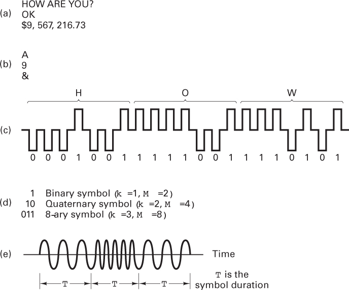
Figure 1.3 Nomenclature examples. (a) Textual messages. (b) Characters. (c) Bit stream (7-bit ASCII). (d) Symbols mi, i = 1,…, M, M = 2k. (e) Bandpass digital waveform si (t), i = 1,…, M.
Character. A character is a member of an alphabet or a set of symbols (see Figure 1.3b). Characters may be mapped into a sequence of binary digits.
Several standardized codes are used for character encoding, including the American Standard Code for Information Interchange (ASCII), Extended Binary Coded Decimal Interchange Code (EBCDIC), Hollerith, Baudot, Murray, and Morse.
Binary digit (bit). This is the fundamental information unit for all digital systems. The term bit also is used as a unit of information content, as described in Chapter 9.
Bit stream. This is a sequence of binary digits (ones and zeros). A bit stream is often termed a baseband signal, which implies that its spectral content extends from (or near) dc up to some finite value, usually less than a few megahertz. In Figure 1.3c, the message “HOW” is represented with the 7-bit ASCII character code, where the bit stream is shown by using a convenient picture of 2-level pulses. The sequence of pulses is drawn using very stylized (ideal-rectangular) shapes with spaces between successive pulses. In a real system, the pulses would never appear as they are depicted here because such spaces would serve no useful purpose. For a given bit rate, the spaces would increase the bandwidth needed for transmission; or, for a given bandwidth, they would increase the time delay needed to receive the message.
Symbol (digital message). A symbol is a group of k bits considered as a unit. We refer to this unit as a message symbol mi (i = 1,…, M) from a finite symbol set or alphabet (see Figure 1.3d). The size of the alphabet, M, is M = 2k, where k is the number of bits in the symbol. For baseband transmission, each mi symbol is represented by one of a set of baseband pulse waveforms g1(t), g2(t),…, gM(t). When transmitting a sequence of such pulses, the unit Baud is sometimes used to express pulse rate (symbol rate). For typical bandpass transmission, each gi(t) pulse is then represented by one of a set of bandpass waveforms s1(t), s2(t),…, sM(t). Thus, for wireless systems, the symbol mi is sent by transmitting the digital waveform si(t) for T seconds, the symbol duration time. The next symbol is sent during the next time interval, T. The fact that the symbol set transmitted by the DCS is finite is a primary difference between a DCS and an analog system. The DCS receiver need only decide which of the M waveforms was transmitted; however, an analog receiver must be capable of accurately estimating a continuous range of waveforms.
Digital waveform. This is a voltage or current waveform (a pulse for baseband transmission or a sinusoid for bandpass transmission) that represents a digital symbol. The waveform characteristics (amplitude, width, and position for pulses or amplitude, frequency, and phase for sinusoids) allow its identification as one of the symbols in the finite symbol alphabet. Figure 1.3e shows an example of a bandpass digital waveform. Even though the waveform is sinusoidal and consequently has an analog appearance, it is called a digital waveform because it is encoded with digital information. In the figure, during each time interval, T, a preassigned frequency indicates the value of a digit.
Data rate. This quantity, in bits per second (bits/s), is given by R = k/ T = (1/T) log2 M bits/s, where k bits identify a symbol from an M = 2k-symbol alphabet, and T is the k-bit symbol duration.
1.1.4 Digital Versus Analog Performance Criteria
A principal difference between analog and digital communication systems has to do with the way in which we evaluate their performance. Analog systems draw their waveforms from a continuum, which therefore forms an infinite set; that is, a receiver must deal with an infinite number of possible waveshapes. The figure of merit for the performance of analog communication systems is a fidelity criterion, such as signal-to-noise ratio, percent distortion, or expected mean square error between the transmitted and received waveforms.
By contrast, a digital communication system transmits signals that represent digits. These digits form a finite set or alphabet, and the set is known a priori to the receiver. A figure of merit for digital communication systems is the probability of incorrectly detecting a digit, or the probability of error (PE).
1.2 Classification of Signals
1.2.1 Deterministic and Random Signals
A signal can be classified as deterministic, meaning that there is no uncertainty with respect to its value at any time, or as random, meaning that there is some degree of uncertainty before the signal actually occurs. Deterministic signals or waveforms are modeled by explicit mathematical expressions, such as x(t) = 5 cos 10t. For a random waveform, it is not possible to write such an explicit expression. However, when examined over a long period, a random waveform, also referred to as a random process, may exhibit certain regularities that can be described in terms of probabilities and statistical averages. Such a model, in the form of a probabilistic description of the random process, is particularly useful for characterizing signals and noise in communication systems.
1.2.2 Periodic and Nonperiodic Signals
A signal x(t) is called periodic in time if there exists a constant T0 > 0 such that
where t denotes time. The smallest value of T0 that satisfies this condition is called the period of x(t). The period T0 defines the duration of one complete cycle of x(t). A signal for which there is no value of T0 that satisfies Equation (1.2) is called a nonperiodic signal.
1.2.3 Analog and Discrete Signals
An analog signal x(t) is a continuous function of time; that is, x(t) is uniquely defined for all t. An electrical analog signal arises when a physical waveform (e.g., speech) is converted into an electrical signal by means of a transducer. By comparison, a discrete signal x(kT) is one that exists only at discrete times; it is characterized by a sequence of numbers defined for each time, kT, where k is an integer and T is a fixed time interval.
1.2.4 Energy and Power Signals
An electrical signal can be represented as a voltage v(t) or a current i(t) with instantaneous power p(t) across a resistor ℜ defined by
or
In communication systems, power is often normalized by assuming ℜ to be 1 Ω, although ℜ may be another value in the actual circuit. If the actual value of the power is needed, it is obtained by “denormalization” of the normalized value. For the normalized case, Equations 1.3a and 1.3b have the same form. Therefore, regardless of whether the signal is a voltage or current waveform, the normalization convention allows us to express the instantaneous power as
where x(t) is either a voltage or a current signal. The energy dissipated during the time interval (–T/2, T/2) by a real signal with instantaneous power expressed by Equation (1.4) can then be written as
and the average power dissipated by the signal during the interval is
The performance of a communication system depends on the received signal energy; higher energy signals are detected more reliably (with fewer errors) than are lower energy signals; the received energy does the work. On the other hand, power is the rate at which energy is delivered. It is important for different reasons. The power determines the voltages that must be applied to a transmitter and the intensities of the electromagnetic fields that one must contend with in radio systems (i.e., fields in waveguides that connect the transmitter to the antenna and fields around the radiating elements of the antenna).
In analyzing communication signals, it is often desirable to deal with the waveform energy. We classify x(t) as an energy signal if, and only if, it has nonzero but finite energy (0 < Ex < ∞) for all time, where
In the real world, we always transmit signals having finite energy (0 < Ex < ∞). However, in order to describe periodic signals, which by definition [Equation (1.2)] exist for all time and thus have infinite energy, and in order to deal with random signals that have infinite energy, it is convenient to define a class of signals called power signals. A signal is defined as a power signal if, and only if, it has finite but nonzero power (0 < Px < ∞) for all time, where
The energy and power classifications are mutually exclusive. An energy signal has finite energy but zero average power, whereas a power signal has finite average power but infinite energy. A waveform in a system may be constrained in either its power or energy values. As a general rule, periodic signals and random signals are classified as power signals, while signals that are both deterministic and nonperiodic are classified as energy signals [1, 2].
Signal energy and power are both important parameters in specifying a communication system. The classification of a signal as either an energy signal or a power signal is a convenient model to facilitate the mathematical treatment of various signals and noise. In Section 3.1.5, these ideas are developed further, in the context of a digital communication system.
1.2.5 The Unit Impulse Function
A useful function in communication theory is the unit impulse function, or Dirac delta function δ(t). The impulse function is an abstraction–an infinitely large amplitude pulse, with zero pulse width and unity weight (area under the pulse), concentrated at the point where its argument is zero. The unit impulse is characterized by the following relationships:
The unit impulse function δ(t) is not a function in the usual sense. When operations involve δ(t), the convention is to interpret δ(t) as a unit area pulse of finite amplitude and nonzero duration, after which the limit is considered as the pulse duration approaches zero. δ(t – t0) can be depicted graphically as a spike located at t = t0 with height equal to its integral or area. Thus Aδ(t – t0) with A constant represents an impulse function whose area or weight is equal to A that is zero everywhere except at t = t0.
Equation (1.12) is known as the sifting, or sampling, property of the unit impulse function; the unit impulse multiplier selects a sample of the function x(t) evaluated at t = t0.
1.3 Spectral Density
The spectral density of a signal characterizes the distribution of the signal’s energy or power in the frequency domain. This concept is particularly important when considering filtering in communication systems. We need to be able to evaluate the signal and noise at the filter output. The energy spectral density (ESD) or the power spectral density (PSD) is used in the evaluation.
1.3.1 Energy Spectral Density
The total energy of a real-valued energy signal x(t), defined over the interval (–∞, ∞), is described by Equation (1.7). Using Parseval’s theorem [1], we can relate the energy of such a signal expressed in the time domain to the energy expressed in the frequency domain, as
where X(f) is the Fourier transform of the nonperiodic signal x(t). (For a review of Fourier techniques, see Appendix A online at informit.com/title/9780134588568.) Let ψx(f) denote the squared magnitude spectrum, defined as
The quantity ψx(f) is the waveform energy spectral density (ESD) of the signal x(t). Therefore, from Equation (1.13), we can express the total energy of x(t) by integrating the spectral density with respect to frequency:
This equation states that the energy of a signal is equal to the area under the ψx(f) versus frequency curve. Energy spectral density describes the signal energy per unit bandwidth measured in joules/hertz. There are equal energy contributions from both positive and negative frequency components, since for a real signal, x(t), |X(f)| is an even function of frequency. Therefore, the energy spectral density is symmetrical in frequency about the origin, and thus the total energy of the signal x(t) can be expressed as
1.3.2 Power Spectral Density
The average power Px of a real-valued power signal x(t) is defined in Equation (1.8). If x(t) is a periodic signal with period T0, it is classified as a power signal. The expression for the average power of a periodic signal takes the form of Equation (1.6), where the time average is taken over the signal period T0, as follows:
Parseval’s theorem for a real-valued periodic signal [1] takes the form
where the cn terms are the complex Fourier series coefficients of the periodic signal. (See Appendix A on the companion website at informit.com/title/9780134588568.)
To apply Equation (1.17b), we need only know the magnitude of the coefficients, |cn|. The power spectral density (PSD) function Gx(f) of the periodic signal x(t) is a real, even, and nonnegative function of frequency that gives the distribution of the power of x(t) in the frequency domain, defined as
Equation (1.18) defines the power spectral density of a periodic signal x(t) as a succession of the weighted delta functions. Therefore, the PSD of a periodic signal is a discrete function of frequency. Using the PSD defined in Equation (1.18), we can now write the average normalized power of a real-valued signal as
Equation (1.18) describes the PSD of periodic (power) signals only. If x(t) is a nonperiodic signal, it cannot be expressed by a Fourier series, and if it is a nonperiodic power signal (having infinite energy), it may not have a Fourier transform. However, we may still express the power spectral density of such signals in the limiting sense. If we form a truncated version xT(t) of the nonperiodic power signal x(t) by observing it only in the interval (–T/2, T/2), then xT(t) has finite energy and has a proper Fourier transform XT(f). It can be shown [2] that the power spectral density of the nonperiodic x(t) can then be defined in the limit as
1.4 Autocorrelation
1.4.1 Autocorrelation of an Energy Signal
Correlation is a matching process; autocorrelation refers to the matching of a signal with a delayed version of itself. The autocorrelation function of a real-valued energy signal x(t) is defined as
The autocorrelation function Rx(τ) provides a measure of how closely the signal matches a copy of itself as the copy is shifted τ units in time. The variable τ plays the role of a scanning or searching parameter. Rx(τ) is not a function of time; it is only a function of the time difference τ between the waveform and its shifted copy.
The autocorrelative function of a real-valued energy signal has the following properties:
1. Rx(τ) = Rx(τ) |
symmetrical in τ about zero |
2. |Rx(τ)| ≤ Rx(0) for all τ |
maximum value occurs at the origin |
3. Rx(τ) ↔ ψx(f) |
autocorrelation and ESD form a Fourier transform pair, as designated by the double-headed arrow |
4. |
value at the origin is equal to the energy of the signal |
If items 1 through 3 are satisfied, Rx(τ) satisfies the properties of an autocorrelation function. Property 4 can be derived from property 3 and thus need not be included as a basic test.
1.4.2 Autocorrelation of a Periodic (Power) Signal
The autocorrelation function of a real-valued power signal x(t) is defined as
When the power signal x(t) is periodic with period T0, the time average in Equation (1.22) may be taken over a single period T0, and the autocorrelation function can be expressed as
The autocorrelation function of a real-valued periodic signal has properties similar to those of an energy signal:
1. Rx(τ) = Rx(–τ) |
symmetrical in τ about zero |
2. |Rx(τ)| ≤ Rx(0) for all τ |
maximum value occurs at the origin |
3. Rx(τ) ↔ Gx(f) |
autocorrelation and PSD form a Fourier transform pair |
4. |
value at the origin is equal to the average power of the signal |
1.5 Random Signals
The main objective of a communication system is the transfer of information over a channel. All useful message signals appear random; that is, the receiver does not know, a priori, which of the possible message waveforms will be transmitted. Also, the noise that accompanies the message signals is due to random electrical signals. Therefore, we need to be able to form efficient descriptions of random signals.
1.5.1 Random Variables
Let a random variable X(A) represent the functional relationship between a random event A and a real number. For notational convenience, we shall designate the random variable X and let the functional dependence upon A be implicit. The random variable may be discrete or continuous. The distribution function FX(x) of the random variable X is given by
where P(X ≤ x) is the probability that the value taken by the random variable X is less than or equal to a real number x. The distribution function FX(x) has the following properties:
0 ≤ FX(x) ≤ 1
FX(x1) ≤ FX(x2) if x1 ≤ x2
FX(– ∞) = 0
FX(+ ∞) = 1
Another useful function related to the random variable X is the probability density function (pdf), denoted as
As in the case of the distribution function, the pdf is a function of a real number x. The name “density function” arises from the fact that the probability of the event x1 ≤ X ≤ x2 equals
From Equation (1.25b), the probability that a random variable X has a value in some very narrow range between x and x + Δx can be approximated as
Thus, in the limit as Δx approaches zero, we can write
The probability density function has the following properties:
pX(x) ≥ 0
Thus, a probability density function is always a nonnegative function with a total area of one. Throughout the book, we use the designation pX(x) for the probability density function of a continuous random variable. For ease of notation, we often omit the subscript X and write simply p(x). We use the designation p(X = xi) for the probability of a random variable X, where X can take on discrete values only.
1.5.1.1 Ensemble Averages
The mean value mX, or expected value of a random variable X, is defined by
where E{·} is called the expected value operator. The nth moment of a probability distribution of a random variable X is defined by
For the purposes of communication system analysis, the most important moments of X are the first two moments. Thus, n = 1 in Equation (1.27) gives mX as discussed above, whereas n = 2 gives the mean square value of X, as follows:
We can also define central moments, which are the moments of the difference between X and mX. The second central moment, called the variance of X, is defined as
The variance of X is also denoted as , and its square root, σX, is called the standard deviation of X. Variance is a measure of the “randomness” of the random variable X. By specifying the variance of a random variable, we are constraining the width of its probability density function. The variance and the mean square value are related by
Thus, the variance is equal to the difference between the mean square value and the square of the mean.
1.5.2 Random Processes
A random process X(A, t) can be viewed as a function of two variables: an event A and time. Figure 1.4 illustrates a random process. In the figure, there are N sample functions of time, {Xj(t)}. Each of the sample functions can be regarded as the output of a different noise generator. For a specific event Aj, we have a single time function X(Aj, t) = Xj(t) (i.e., a sample function). The totality of all sample functions is called an ensemble. For a specific time tk, X(A, tk) is a random variable X(tk) whose value depends on the event. Finally, for a specific event A = Aj and a specific time t = tk, X(Aj, tk) is simply a number. For notational convenience, we shall designate the random process by X(t) and let the functional dependence upon A be implicit.
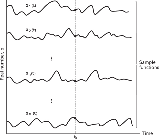
Figure 1.4 Random noise process.
1.5.2.1 Statistical Averages of a Random Process
Because the value of a random process at any future time is unknown (since the identity of the event A is unknown), a random process whose distribution functions are continuous can be described statistically with a probability density function (pdf). In general, the form of the pdf of a random process will be different for different times. In most situations, it is not practical to determine empirically the probability distribution of a random process. However, a partial description consisting of the mean and autocorrelation function is often adequate for the needs of a communication system. We define the mean of the random process X(t) as
where X(tk) is the random variable obtained by observing the random process at time tk and the pdf of X(tk), the density over the ensemble of events at time tk, is designated pXk(x).
We define the autocorrelation function of the random process X(t) to be a function of two variables, t1 and t2, given by
where X(t1) and X(t2) are random variables obtained by observing X(t) at times t1 and t2, respectively. The autocorrelation function is a measure of the degree to which two time samples of the same random process are related.
1.5.2.2 Stationarity
A random process X(t) is said to be stationary in the strict sense if none of its statistics are affected by a shift in the time origin. A random process is said to be wide-sense stationary (WSS) if two of its statistics, its mean and autocorrelation function, do not vary with a shift in the time origin. Thus, a process is WSS if
and
Strict-sense stationary implies wide-sense stationary but not vice versa. Most of the useful results in communication theory are predicated on random information signals and noise being wide-sense stationary. From a practical point of view, it is not necessary for a random process to be stationary for all time but only for some observation interval of interest.
For stationary processes, the autocorrelation function in Equation (1.33) does not depend on time but only on the difference between t1 and t2. That is, all pairs of values of X(t) at points in time separated by τ = t1 – t2 have the same correlation value. Thus, for stationary systems, we can denote RX(t1, t2) simply as RX(τ).
1.5.2.3 Autocorrelation of a Wide-Sense Stationary Random Process
Just as the variance provides a measure of randomness for random variables, the autocorrelation function provides a similar measure for random processes. For a wide-sense stationary process, the autocorrelation function is only a function of the time difference τ = t1 – t2; that is,
For a zero mean WSS process, RX(τ) indicates the extent to which the random values of the process separated by τ seconds in time are statistically correlated. In other words, RX(τ) gives us an idea of the frequency response that is associated with a random process. If RX(τ) changes slowly as τ increases from zero to some value, it indicates that, on average, sample values of X(t) taken at t = t1 and t = t1 + τ are nearly the same. Thus, we would expect a frequency domain representation of X(t) to contain a preponderance of low frequencies. On the other hand, if RX(τ) decreases rapidly as τ is increased, we would expect X(t) to change rapidly with time and thereby contain mostly high frequencies.
Properties of the autocorrelation function of a real-valued wide-sense stationary process are as follows:
1. RX(τ) = RX(–τ) |
symmetrical in τ about zero |
2. |RX(τ)| ≤ RX(0) for all τ |
maximum value occurs at the origin |
3. RX(τ) ↔ GX(f) |
autocorrelation and power spectral density form a Fourier transform pair |
4. RX(0) = E{X2(t)} |
value at the origin is equal to the average power of the signal |
1.5.3 Time Averaging and Ergodicity
To compute mX and RX(τ) by ensemble averaging, we would have to average across all the sample functions of the process and would need to have complete knowledge of the first- and second-order joint probability density functions. Such knowledge is generally not available.
When a random process belongs to a special class, known as an ergodic process, its time averages equal its ensemble averages, and the statistical properties of the process can be determined by time averaging over a single sample function of the process. For a random process to be ergodic, it must be stationary in the strict sense. (The converse is not necessary.) However, for communication systems, where we are satisfied to meet the conditions of wide-sense stationarity, we are interested only in the mean and autocorrelation functions.
We can say that a random process is ergodic in the mean if
and it is ergodic in the autocorrelation function if
Testing for the ergodicity of a random process is usually very difficult. In practice, one makes an intuitive judgment as to whether it is reasonable to interchange the time and ensemble averages. A reasonable assumption in the analysis of most communication signals (in the absence of transient effects) is that the random waveforms are ergodic in the mean and the autocorrelation function. Since time averages equal ensemble averages for ergodic processes, fundamental electrical engineering parameters, such as dc value, root mean square (rms) value, and average power can be related to the moments of an ergodic random process. Following is a summary of these relationships:
The quantity mX = E{X(t)} is equal to the dc level of the signal.
The quantity is equal to the normalized power in the dc component.
The second moment of X(t), E{X2(t)}, is equal to the total average normalized power.
The quantity is equal to the rms value of the voltage or current signal.
The variance is equal to the average normalized power in the time-varying or ac component of the signal.
If the process has zero mean (i.e., ), then , and the variance is the same as the mean square value, or the variance represents the total power in the normalized load.
The standard deviation σX is the rms value of the ac component of the signal.
If mX = 0, then σX is the rms value of the signal.
1.5.4 Power Spectral Density and Autocorrelation of a Random Process
A random process X(t) can generally be classified as a power signal having a power spectral density (PSD) GX(f) of the form shown in Equation (1.20). GX(f) is particularly useful in communication systems because it describes the distribution of a signal’s power in the frequency domain. The PSD enables us to evaluate the signal power that will pass through a network having known frequency characteristics. We summarize the principal features of PSD functions as follows:
1. GX(f) ≥ 0 |
and is always real valued |
2. GX(f) = GX(– f) |
for X(t) real valued |
3. GX(f) ↔ RX(τ) |
PSD and autocorrelation form a Fourier transform pair |
4. |
relationship between average normalized power and PSD |
In Figure 1.5, we present a visualization of autocorrelation and power spectral density functions. What does the term correlation mean? When we inquire about the correlation between two phenomena, we are asking how closely they correspond in behavior or appearance, how well they match one another. In mathematics, an autocorrelation function of a signal (in the time domain) describes the correspondence of the signal to itself in the following way: An exact copy of the signal is made and located in time at minus infinity. Then we move the copy an increment in the direction of positive time and ask the question, “How well do these two (the original and the copy) match”? We move the copy another step in the positive direction and ask, “How well do they match now?” And so forth. The correlation between the two is plotted as a function of time, denoted τ, which can be thought of as a scanning parameter.
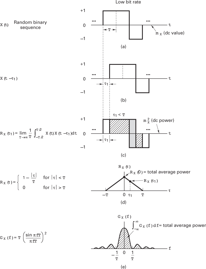

Figure 1.5 Autocorrelation and power spectral density.
Figure 1.5a–d highlights some of these steps. Figure 1.5a illustrates a single sample waveform from a WSS random process, X(t). The waveform is a binary random sequence with unit-amplitude positive and negative (bipolar) pulses. The positive and negative pulses occur with equal probability. The duration of each binary digit is T seconds, and the average or dc value of the random sequence is zero. Figure 1.5b shows the same sequence displaced τ1 seconds in time; this sequence is therefore denoted X(t – τ1). Let us assume that X(t) is ergodic in the autocorrelation function so that we can use time averaging instead of ensemble averaging to find RX(τ). The value of RX(τ1) is obtained by taking the product of the two sequences X(t) and X(t – τ1) and finding the average value using Equation (1.36). Equation (1.36) is accurate for ergodic processes only in the limit. However, integration over an integer number of periods can provide us with an estimate of RX(τ). Notice that RX(τ1) can be obtained by a positive or negative shift of X(t). Figure 1.5c illustrates such a calculation, using the single sample sequence (Figure 1.5a) and its shifted replica (Figure 1.5b). The cross-hatched areas under the product curve X(t)X(t – τ1) contribute to positive values of the product, and the gray areas contribute to negative values. The integration of X(t) X(t – τ1) over several pulse times yields a net value of area which is one point, the RX(τ1) point of the RX(τ) curve. The sequences can be further shifted by τ2, τ3,…, each shift yielding a point on the overall autocorrelation function RX(τ) shown in Figure 1.5d. Every random sequence of bipolar pulses has an autocorrelation plot of the general shape shown in Figure 1.5d. The plot peaks at RX(0) [the best match occurs when τ equals zero, since R(τ) ≤ R(0) for all τ], and it declines as τ increases. Figure 1.5d shows points corresponding to RX(0) and RX(τ1).
The analytical expression for the autocorrelation function RX(τ) shown in Figure 1.5d is [1]
Notice that the autocorrelation function gives us frequency information; it tells us something about the bandwidth of the signal. Autocorrelation is a time-domain function; there are no frequency-related terms in the relationship shown in Equation (1.37). How does it give us bandwidth information about the signal? Consider that the signal is a very slowly moving (low-bandwidth) signal. As we step the copy along the τ axis, at each step asking the question, “How good is the match between the original and the copy?” the match will be quite good for a while. In other words, the triangular-shaped autocorrelation function in Figure 1.5d and Equation (1.37) will ramp down gradually with τ. But if we have a very rapidly moving (high-bandwidth) signal, perhaps a very small shift in τ will result in there being zero correlation. In this case, the autocorrelation function will have a very steep appearance. Therefore, the relative shape of the autocorrelation function tells us something about the bandwidth of the underlying signal. Does it ramp down gently? If so, then we are dealing with a low-bandwidth signal. Is the function steep? If so, then we are dealing with a high-bandwidth signal.
The autocorrelation function allows us to express a random signal’s power spectral density directly. Since the PSD and the autocorrelation function are Fourier transforms of each other, the PSD, GX(f), of the random bipolar-pulse sequence can be found using Table A.1 as the transform of RX(τ) in Equation (1.37). Observe that
where
The general shape of GX(f) is illustrated in Figure 1.5e.
Notice that the area under the PSD curve represents the average power in the signal. One convenient measure of bandwidth is the width of the main spectral lobe. (See Section 1.7.2.) Figure 1.5e illustrates that the bandwidth of a signal is inversely related to the symbol duration or pulse width, Figures 1.5f–j repeat the steps shown in Figures 1.5a–e, except that the pulse duration is shorter. Notice that the shape of the shorter pulse duration RX(τ) is narrower, shown in Figure 1.5i, than it is for the longer pulse duration RX(τ), shown in Figure 1.5d. In Figure 1.5i, RX(τ1) = 0; in other words, a shift of τ1 in the case of the shorter pulse duration example is enough to produce a zero match, or a complete decorrelation between the shifted sequences. Since the pulse duration T is shorter (pulse rate is higher) in Figure 1.5f than in Figure 1.5a, the bandwidth occupancy in Figure 1.5j is greater than the bandwidth occupancy shown in Figure 1.5e for the lower pulse rate.
1.5.5 Noise in Communication Systems
The term noise refers to unwanted electrical signals that are always present in electrical systems. The presence of noise superimposed on a signal tends to obscure or mask the signal; it limits the receiver’s ability to make correct symbol decisions, and thereby limits the rate of information transmission. Noise arises from a variety of sources, both human created and natural. Human-created noise includes such sources as spark-plug ignition noise, switching transients, and other radiating electromagnetic signals. Natural noise includes such elements as the atmosphere, the sun, and other galactic sources.
Good engineering design can eliminate much of the noise or its undesirable effect through filtering, shielding, the choice of modulation, and the selection of an optimum receiver site. For example, sensitive radio astronomy measurements are typically located at remote desert locations, far from human-created noise sources. However, there is one natural source of noise, called thermal noise, or Johnson noise, that cannot be eliminated. Thermal noise [4, 5] is caused by the thermal motion of electrons in all dissipative components–resistors, wires, and so on. The same electrons that are responsible for electrical conduction are also responsible for thermal noise.
We can describe thermal noise as a zero-mean Gaussian random process. A Gaussian process n(t) is a random function whose value n at any arbitrary time t is statistically characterized by the Gaussian probability density function
where σ2 is the variance of n. The normalized or standardized Gaussian density function of a zero-mean process is obtained by assuming that σ = 1. This normalized pdf is shown sketched in Figure 1.6.
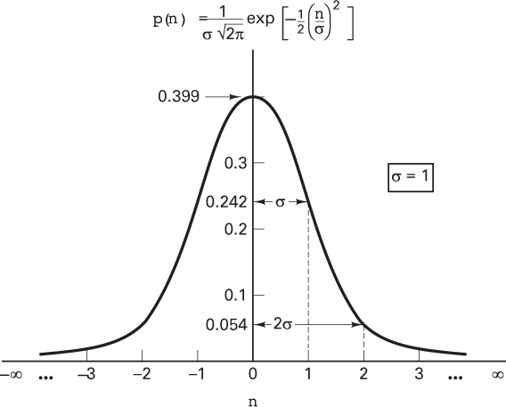
Figure 1.6 Normalized (σ = 1) Gaussian probability density function.
We often represent a random signal as the sum of a Gaussian noise random variable and a dc signal. That is,
z = a + n
where z is the random signal, a is the dc component, and n is the Gaussian noise random variable. The pdf p(z) is then expressed as
where, as before, σ2 is the variance of n. The Gaussian distribution is often used as the system noise model because of a theorem, called the central limit theorem [3], which states that under very general conditions, the probability distribution of the sum of j statistically independent random variables approaches the Gaussian distribution as j → ∞, no matter what the individual distribution functions may be. Therefore, even though individual noise mechanisms might have other than Gaussian distributions, the aggregate of many such mechanisms tends toward the Gaussian distribution.
1.5.5.1 White Noise
The primary spectral characteristic of thermal noise is that its power spectral density is the same for all frequencies of interest in most communication systems; in other words, a thermal noise source emanates an equal amount of noise power per unit bandwidth at all frequencies–from dc to about 1012 Hz. Therefore, a simple model for thermal noise assumes that its power spectral density Gn(f) is flat for all frequencies, as shown in Figure 1.7a, and is denoted as
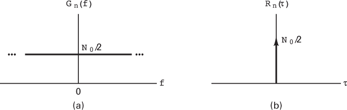
Figure 1.7 (a) Power spectral density of white noise. (b) Autocorrelation function of white noise.
where the factor of 2 is included to indicate that Gn(f) is a two-sided power spectral density. When the noise power has such a uniform spectral density, we refer to it as white noise, where the adjective white is used in the same sense as it is with white light, which contains equal amounts of all frequencies within the visible band of electromagnetic radiation.
The autocorrelation function of white noise is given by the inverse Fourier transform of the noise power spectral density (see Table A.1), denoted as follows:
Thus the autocorrelation of white noise is a delta function weighted by the factor N0/2 and occurring at τ = 0, as seen in Figure 1.7b. Note that Rn(τ) is zero for τ ≠ 0; that is, any two different samples of white noise, no matter how close together in time they are taken, are uncorrelated.
The average power Pn of white noise is infinite because its bandwidth is infinite. This can be seen by combining Equations (1.19) and (1.42) to yield
Although white noise is a useful abstraction, no noise process can truly be white; however, the noise encountered in many real systems can be assumed to be approximately white. We can only observe such noise after it has passed through a real system that has a finite bandwidth. Thus, as long as the bandwidth of the noise is appreciably larger than that of the system, the noise can be considered to have an infinite bandwidth.
The delta function in Equation (1.43) means that the noise signal n(t) is totally decorrelated from its time-shifted version for any τ > 0. Equation (1.43) indicates that any two different samples of a white noise process are uncorrelated. Since thermal noise is a Gaussian process and the samples are uncorrelated, the noise samples are also independent [3]. Therefore, the effect on the detection process of a channel with additive white Gaussian noise (AWGN) is that the noise affects each transmitted symbol independently. Such a channel is called a memoryless channel. The term additive means that the noise is simply superimposed or added to the signal; that there are no multiplicative mechanisms at work.
Since thermal noise is present in all communication systems and is the prominent noise source for most systems, the thermal noise characteristics–additive, white, and Gaussian–are most often used to model the noise in communication systems. Since zero-mean Gaussian noise is completely characterized by its variance, this model is particularly simple to use in the detection of signals and in the design of optimum receivers. In this book we assume, unless otherwise stated, that the system is corrupted by additive zero-mean white Gaussian noise, even though this is sometimes an oversimplification.
1.6 Signal Transmission Through Linear Systems
Having developed a set of models for signals and noise, we now consider the characterization of systems and their effects on such signals and noise. Since a system can be characterized equally well in the time domain or the frequency domain, techniques will be developed in both domains to analyze the response of a linear system to an arbitrary input signal. The signal, applied to the input of the system, as shown in Figure 1.8, can be described either as a time-domain signal, x(t), or by its Fourier transform, X(f ). The use of time-domain analysis yields the time-domain output y(t), and in the process, h(t), the characteristic, or impulse response, of the network will be defined. When the input is considered in the frequency domain, we shall define a frequency transfer function H(f ) for the system, which will determine the frequency-domain output Y(f ). The system is assumed to be linear and time invariant. It is also assumed that there is no stored energy in the system at the time the input is applied.

Figure 1.8 Linear system and its key parameters.
1.6.1 Impulse Response
The linear time invariant system or network illustrated in Figure 1.8 is characterized in the time domain by an impulse response h(t), which is the response when the input is equal to a unit impulse δ(t); that is,
Consider the name impulse response. That is a very appropriate name for this event. Characterizing a linear system in terms of its impulse response has a straightforward physical interpretation. At the system input, we apply a unit impulse (a nonrealizable signal, having infinite amplitude, zero width, and unit area), as illustrated in Figure 1.9a. Applying such an impulse to the system can be thought of as giving the system “a whack.” How does the system respond to such a force (impulse) at the input? The output response h(t) is the system’s impulse response. (A possible shape is depicted in Figure 1.9b.)
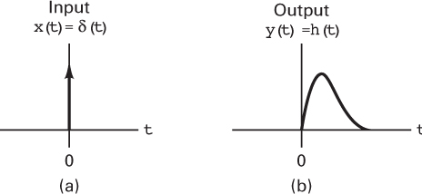
Figure 1.9 (a) Input signal x(t ) is a unit impulse function. (b) Output signal y(t ) is the system’s impulse response h(t).
The response of the network to an arbitrary input signal x(t) is found by the convolution of x(t) with h(t), expressed as
where * denotes the convolution operation. (See Section A.5.) The system is assumed to be causal, which means that there can be no output prior to the time, t = 0, when the input is applied. Therefore, the lower limit of integration can be changed to zero, and we can express the output y(t) in either the form
or the form
Each of the expressions in Equations (1.46) and (1.47) is called the convolution integral. Convolution is a basic mathematical tool that plays an important role in understanding all communication systems. Thus, the reader is urged to review Section A.5, where one can see that Equations (1.46) and (1.47) are the results of a straightforward process.
1.6.2 Frequency Transfer Function
The frequency-domain output signal Y(f ) is obtained by taking the Fourier transform of both sides of Equation (1.46). Since convolution in the time domain transforms to multiplication in the frequency domain (and vice versa), Equation (1.46) yields
or
provided, of course, that X(f) ≠ 0 for all f. Here H(f) = ℱ{h(t)}, the Fourier transform of the impulse response function, is called the frequency transfer function or the frequency response of the network. In general, H(f) is complex and can be written as
where |H(f)| is the magnitude response. The phase response is defined as
where the terms Re and Im denote “the real part of” and “the imaginary part of,” respectively.
The frequency transfer function of a linear time-invariant network can easily be measured in the laboratory with a sinusoidal generator at the input of the network and an oscilloscope at the output. When the input waveform x(t) is expressed as
x(t) = A cos 2πf0t
the output of the network will be
The input frequency f0 is stepped through the values of interest; at each step, the amplitude and phase at the output are measured.
1.6.2.1 Random Processes and Linear Systems
If a random process forms the input to a time-invariant linear system, the output will also be a random process. That is, each sample function of the input process yields a sample function of the output process. The input power spectral density GX(f) and the output power spectral density GY(f) are related as follows:
Equation (1.53) provides a simple way of finding the power spectral density out of a time-invariant linear system when the input is a random process.
In Chapters 3 and 4 we consider the detection of signals in Gaussian noise. We will utilize a fundamental property of a Gaussian process applied to a linear system, as follows. It can be shown that if a Gaussian process X(t) is applied to a time-invariant linear filter, the random process Y(t) developed at the output of the filter is also Gaussian [6].
1.6.3 Distortionless Transmission
What is required of a network for it to behave like an ideal transmission line? The output signal from an ideal transmission line may have some time delay compared with the input, and it may have a different amplitude than the input (just a scale change), but otherwise it must have no distortion; it must have the same shape as the input. Therefore, for ideal distortionless transmission, we can describe the output signal as
where K and t0 are constants. Taking the Fourier transform of both sides (see Section A.3.1), we write
Substituting the expression (1.55) for Y(f) into Equation (1.49), we see that the required system transfer function for distortionless transmission is
Therefore, to achieve ideal distortionless transmission, the overall system response must have a constant magnitude response, and its phase shift must be linear with frequency. It is not enough that the system amplify or attenuate all frequency components equally. All of the signal’s frequency components must also arrive with identical time delay in order to add up correctly. Since the time delay t0 is related to the phase shift θ and the radian frequency ω = 2πf by
it is clear that phase shift must be proportional to frequency in order for the time delay of all components to be identical. A characteristic often used to measure delay distortion of a signal is called envelope delay, or group delay, defined as
Therefore, for distortionless transmission, an equivalent way of characterizing phase to be a linear function of frequency is to characterize the envelope delay τ(f) as a constant. In practice, a signal will be distorted in passing through some parts of a system. Phase or amplitude correction (equalization) networks may be introduced elsewhere in the system to correct for this distortion. It is the overall input/output characteristic of the system that determines its performance.
1.6.3.1 Ideal Filter
One cannot build the ideal network described in Equation (1.56). The problem is that Equation (1.56) implies an infinite bandwidth capability, where the bandwidth of a system is defined as the interval of positive frequencies over which the magnitude |H(f)| remains within a specified value. In Section 1.7 various measures of bandwidth are enumerated. As an approximation to the ideal infinite-bandwidth network, let us choose a truncated network that passes, without distortion, all frequency components between fℓ and fu, where fℓ is the lower cutoff frequency and fu is the upper cutoff frequency, as shown in Figure 1.10. Each of these networks is called an ideal filter. Outside the range fℓ < f < fu, which is called the passband, the ideal filter is assumed to have a response of zero magnitude. The effective width of the passband is specified by the filter bandwidth Wf = (fu – fℓ) hertz.
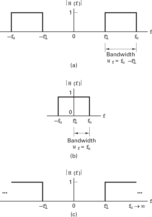
Figure 1.10 Ideal filter transfer function. (a) Ideal bandpass filter. (b) Ideal low-pass filter. (c) Ideal high-pass filter.
When fℓ ≠ 0 and fu ≠ ∞, the filter is called a bandpass filter (BPF), shown in Figure 1.10a. When fℓ = 0 and fu has a finite value, the filter is called a low-pass filter (LPF), shown in Figure 1.10b. When fℓ has a nonzero value and when fu → ∞, the filter is called a high-pass filter (HPF), shown in Figure 1.10c.
Following Equation (1.56) and letting K = 1, for the ideal low-pass filter transfer function with bandwidth Wf = fu hertz, shown in Figure 1.10b, we can write the transfer function as
where
and
The impulse response of the ideal low-pass filter, illustrated in Figure 1.11, is

Figure 1.11 Impulse response of the ideal low-pass filter.
or
where sinc x is as defined in Equation (1.39). The impulse response shown in Figure 1.11 is noncausal, which means it has a nonzero output prior to the application of an input at time t = 0. Therefore, it should be clear that the ideal filter described in Equation (1.58) is not realizable.
1.6.3.2 Realizable Filters
The very simplest example of a realizable low-pass filter is made up of resistance (ℜ) and capacitance (C), as shown in Figure 1.12a; it is called an ℜC filter, and its transfer function can be expressed as [7]

Figure 1.12 ℜC filter and its transfer function. (a) ℜC filter. (b) Magnitude characteristic of the ℜC filter. (c) Phase characteristic of the ℜC filter.
where θ(f) = tan–1 2πfℜC. The magnitude characteristic |H(f)| and the phase characteristic θ(f) are plotted in Figures 1.12b and c, respectively. The low-pass filter bandwidth is defined to be its half-power point; this point is the frequency at which the output signal power has fallen to one-half of its peak value, or the frequency at which the magnitude of the output voltage has fallen to of its peak value.
The half-power point is generally expressed in decibel (dB) units as the –3 dB point, or the point that is 3 dB down from the peak, where the decibel is defined as the ratio of two amounts of power, P1 and P2, existing at two points. By definition,
where V1 and V2 are voltages, and ℜ1 and ℜ2 are resistances. For communication systems, normalized power is generally used for analysis; in this case, ℜ1 and ℜ2 are set equal to 1 Ω, so that
The amplitude response can be expressed in decibels by
where V1 and V2 are the input and output voltages, respectively, and where the input and output resistances have been assumed equal.
From Equation (1.63), it is easy to verify that the half-power point of the low-pass ℜC filter corresponds to ω = 1/ℜC radians per second or f = 1/(2πℜC) hertz. Thus the bandwidth Wf in hertz is 1/(2πℜC). The filter shape factor is a measure of how well a realizable filter approximates the ideal filter. It is typically defined as the ratio of the filter bandwidths at the –60 dB and –6 dB amplitude response points. A sharp-cutoff bandpass filter can be made with a shape factor as low as about 2. By comparison, the shape factor of the simple ℜC low-pass filter is almost 600.
There are several useful approximations to the ideal low-pass filter characteristic. One of these, the Butterworth filter, approximates the ideal low-pass filter with the function
where fu is the upper –3 db cutoff frequency, and n is referred to as the order of the filter. The higher the order, the greater will be the complexity and the cost to implement the filter. The magnitude function, |H(f)|, is sketched (single sided) for several values of n in Figure 1.13. Note that as n gets larger, the magnitude characteristics approach that of the ideal filter. Butterworth filters are popular because they are the best approximation to the ideal, in the sense of maximal flatness in the filter passband.
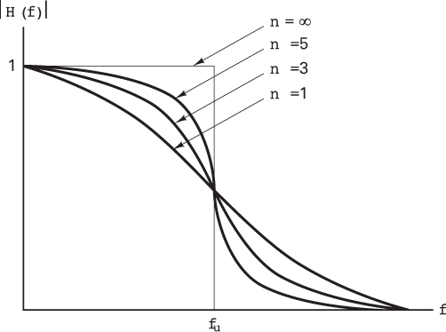
Figure 1.13 Butterworth filter magnitude response.
1.6.4 Signals, Circuits, and Spectra
Signals have been described in terms of their spectra. Similarly, networks or circuits have been described in terms of their spectral characteristics or frequency transfer functions. How is a signal’s bandwidth affected as a result of the signal passing through a filter circuit? Figure 1.14 illustrates two cases of interest. In Figure 1.14a (case 1), the input signal has a narrowband spectrum, and the filter transfer function is a wideband function. From Equation (1.48), we see that the output signal spectrum is simply the product of these two spectra. In Figure 1.14a, we can verify that multiplication of the two spectral functions will result in a spectrum with a bandwidth approximately equal to the smaller of the two bandwidths (when one of the two spectral functions goes to zero, the multiplication yields zero). Therefore, for case 1, the output signal spectrum is constrained by the input signal spectrum alone. Similarly, we see that for case 2, in Figure 1.14b, where the input signal is a wideband signal but the filter has a narrowband transfer function, the bandwidth of the output signal is constrained by the filter bandwidth; the output signal is a filtered (distorted) rendition of the input signal.

Figure 1.14 Spectral characteristics of the input signal and the circuit contribute to the spectral characteristics of the output signal. (a) Case 1: Output bandwidth is constrained by input signal bandwidth. (b) Case 2: Output bandwidth is constrained by filter bandwidth.
The effect of a filter on a waveform can also be viewed in the time domain. The output y(t) resulting from convolving an ideal input pulse x(t) (having amplitude Vm and pulse width T) with the impulse response of a low-pass ℜC filter can be written as [8]
where
Let us define the pulse bandwidth as
and the ℜC filter bandwidth as
The ideal input pulse x(t) and its magnitude spectrum |X(f)| are shown in Figure 1.15. The ℜC filter and its magnitude characteristic |H(f)| are shown in Figures 1.12a and b, respectively. Following Equations (1.66) to (1.69), three cases are illustrated in Figure 1.16. Example 1 illustrates the case where Wp ≪ Wf. Notice that the output response y(t) is a reasonably good approximation of the input pulse x(t), shown in dashed lines. This represents an example of good fidelity. In example 2, where Wp ≈ Wf, we can still recognize that a pulse had been transmitted from the output y(t). Finally, example 3 illustrates the case in which Wp ≫ Wf. Here the presence of the pulse is barely perceptible from y(t). Can you think of an application where the large filter bandwidth or good fidelity of example 1 is called for? A precise ranging application, perhaps, where the pulse time of arrival translates into distance, necessitates a pulse with a steep rise time. Which example characterizes the binary digital communications application? It is example 2. As we pointed out earlier regarding Figure 1.1, one of the principal features of binary digital communications is that each received pulse need only be accurately perceived as being in one of its two states; a high-fidelity signal need not be maintained. Example 3 has been included for completeness; it would not be used as a design criterion for a practical system.

Figure 1.15 (a) Ideal pulse. (b) Magnitude spectrum of the ideal pulse.

Figure 1.16 Three examples of filtering an ideal pulse. (a) Example 1: Good-fidelity output. (b) Example 2: Good-recognition output. (c) Example 3: Poor-recognition output.
1.7 Bandwidth of Digital Data
1.7.1 Baseband Versus Bandpass
An easy way to translate the spectrum of a low-pass or baseband signal x(t) to a higher frequency is to multiply or heterodyne the baseband signal with a carrier wave cos 2πfct, as shown in Figure 1.17. The resulting waveform, xc(t), is called a double-sideband (DSB) modulated signal and is expressed as

Figure 1.17 Comparison of baseband and double-sideband spectra. (a) Heterodyning. (b) Baseband spectrum. (c) Double-sideband spectrum.
From the frequency shifting theorem (see Section A.3.2), the spectrum of the DSB signal xc(t) is given by
The magnitude spectrum |X(f)| of the baseband signal x(t) having a bandwidth fm and the magnitude spectrum |Xc(f)| of the DSB signal xc(t) having a bandwidth WDSB are shown in Figures 1.17b and 1.17c, respectively. In the plot of |Xc(f)|, spectral components corresponding to positive baseband frequencies appear in the range fc to (fc + fm). This part of the DSB spectrum is called the upper sideband (USB). Spectral components corresponding to negative baseband frequencies appear in the range (fc – fm) to fc. This part of the DSB spectrum is called the lower sideband (LSB). Mirror images of the USB and LSB spectra appear in the negative-frequency half of the plot. The carrier wave is sometimes referred to as a local oscillator (LO) signal, a mixing signal, or a heterodyne signal. Generally, the carrier wave frequency is much higher than the bandwidth of the baseband signal; that is,
fc ≫ fm
From Figure 1.17, we can readily compare the bandwidth fm required to transmit the baseband signal with the bandwidth WDSB required to transmit the DSB signal; we see that
That is, we need twice as much transmission bandwidth to transmit a DSB version of the signal as we do to transmit its baseband counterpart.
1.7.2 The Bandwidth Dilemma
Many important theorems of communication and information theory are based on the assumption of strictly bandlimited channels, which means that no signal power whatever is allowed outside the defined band. We are faced with the dilemma that strictly bandlimited signals, as depicted by the spectrum |X1(f)| in Figure 1.18b, are not realizable because they imply signals with infinite duration, as seen by x1(t) in Figure 1.18a (the inverse Fourier transform of X1(f)). Duration-limited signals, as seen by x2(t) in Figure 1.18c, can clearly be realized. However, such signals are just as unreasonable since their Fourier transforms contain energy at arbitrarily high frequencies, as depicted by the spectrum |X2(f)| in Figure 1.18d. In summary, for all bandlimited spectra, the waveforms are not realizable, and for all realizable waveforms, the absolute bandwidth is infinite. The mathematical description of a real signal does not permit the signal to be strictly duration limited and strictly bandlimited. Hence, the mathematical models are abstractions; it is no wonder that there is no single universal definition of bandwidth.
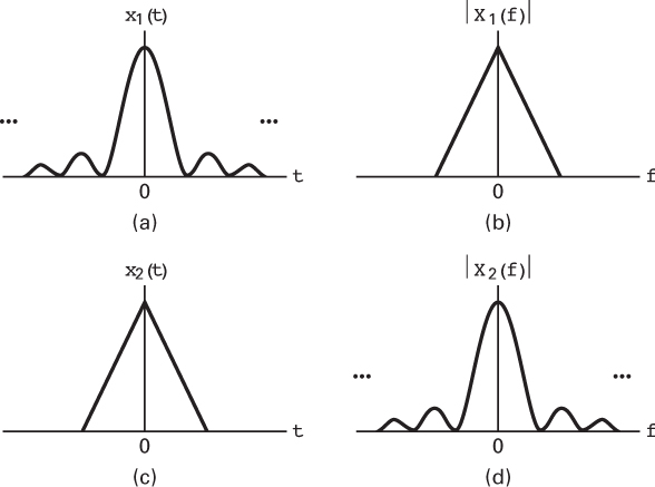
Figure 1.18 (a) Strictly bandlimited signal in the time domain. (b) In the frequency domain. (c) Strictly time limited signal in the time domain. (d) In the frequency domain.
All bandwidth criteria have in common the attempt to specify a measure of the width, W, of a nonnegative real-valued spectral density defined for all frequencies | f| < ∞. Figure 1.19 illustrates some of the most common definitions of bandwidth; in general, the various criteria are not interchangeable. The single-sided power spectral density for a single heterodyned pulse xc(t) takes the analytical form
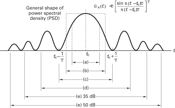
Figure 1.19 Bandwidth of digital data. (a) Half-power. (b) Noise equivalent. (c) Null to null. (d) 99% of power. (e) Bounded PSD (defines attenuation outside bandwidth) at 35 and 50 dB.
where fc is the carrier wave frequency and T is the pulse duration. This power spectral density, whose general appearance is sketched in Figure 1.19, also characterizes a random pulse sequence, assuming that the averaging time is long relative to the pulse duration. The plot consists of a main lobe and smaller symmetrical sidelobes. The general shape of the plot is valid for most digital modulation formats; some formats, however, do not have well-defined lobes. The bandwidth criteria depicted in Figure 1.19 are as follows:
Half-power bandwidth. This is the interval between frequencies at which Gx(f) has dropped to half-power, or 3 dB below the peak value.
Equivalent rectangular or noise equivalent bandwidth, WN. This bandwidth is defined by the relationship WN = Px/Gx(fc), where Px is the total signal power over all frequencies and Gx(fc) is the maximum value (assumed at the band center) of Gx(f ). WN is the bandwidth of a fictitious (ideal rectangular) filter, with the same band-center gain as an actual system, that would pass as much white-noise power as the actual system. The concept of WN facilitates describing or comparing practical linear systems by using idealized equivalents.
Null-to-null bandwidth. The most popular measure of bandwidth for digital communications is the width of the main spectral lobe, where most of the signal power is contained. This criterion lacks complete generality since some modulation formats lack well-defined lobes.
Fractional power containment bandwidth. This bandwidth criterion has been adopted by the Federal Communications Commission (FCC Rules and Regulations Section 2.202) and states that the occupied bandwidth is the band that leaves exactly 0.5% of the signal power above the upper band limit and exactly 0.5% of the signal power below the lower band limit. Thus 99% of the signal power is inside the occupied band.
Bounded power spectral density. A popular method of specifying bandwidth is to state that everywhere outside the specified band, Gx(f) must have fallen at least to a certain stated level below that found at the band center. Typical attenuation levels might be 35 or 50 dB.
Absolute bandwidth. This is the interval between frequencies, outside which the spectrum is zero. This is a useful abstraction. However, for all realizable waveforms, the absolute bandwidth is infinite.
1.8 Conclusion
This chapter has outlined the goals of the book and defined the basic nomenclature. It has also reviewed the fundamental concepts of time-varying signals, such as classification, spectral density, and autocorrelation. It has also considered random signals and characterized white Gaussian noise, the primary noise model in most communication systems, statistically and spectrally. Finally, we have treated the important area of signal transmission through linear systems and have examined some of the realizable approximations to the ideal case. We have also established that the concept of an absolute bandwidth is an abstraction and that in the real world, we are faced with the need to choose a definition of bandwidth that is useful for our particular application. The remainder of the book explores each of the signal processing steps introduced in this chapter in the context of the typical system block diagram appearing at the beginning of each chapter.
References
1. Haykin, S., Communication Systems, John Wiley & Sons, Inc., New York, 1983.
2. Shanmugam, K. S., Digital and Analog Communication Systems, John Wiley & Sons, Inc., New York, 1979.
3. Papoulis, A., Probability, Random Variables, and Stochastic Processes, McGraw-Hill Book Company, New York, 1965.
4. Johnson, J. B., “Thermal Agitation of Electricity in Conductors,” Phys. Rev., vol. 32, July 1928, pp. 97–109.
5. Nyguist, H., “Thermal Agitation of Electric Charge in Conductors,” Phys. Rev., vol. 32, July 1928, pp. 110–113.
6. Van Trees, H. L., Detection, Estimation, and Modulation Theory, Part 1, John Wiley & Sons, New York, 1968.
7. Schwartz, M., Information Transmission, Modulation, and Noise, McGraw-Hill Book Company, New York, 1970.
8. Millman, J., and Taub, H., Pulse, Digital, and Switching Waveforms, McGraw-Hill Book Company, New York, 1965.
Problems
1.1. Classify the following signals as energy signals or power signals. Find the normalized energy or normalized power of each.
1.2. Determine the energy spectral density of a square pulse x(t) = rect (t/T), where rect (t/T) equals 1, for –T/2 ≤ t ≤ T/2, and equals 0 elsewhere. Calculate the normalized energy Ex in the pulse.
1.3. Find an expression for the average normalized power in a periodic signal in terms of its complex Fourier series coefficients.
1.4. Using time averaging, find the average normalized power in the waveform x(t) = 10 cos 10t + 20 cos 20t.
1.5. Repeat Problem 1.4 using the summation of spectral coefficients.
1.6. Determine which, if any, of the following functions have the properties of autocorrelation functions. Justify your determination. [Note: {R(τ)} must be a nonnegative function. Why?]
x(τ) = δ(τ) + sin 2πf0τ
x(τ) = exp (|τ|)
x(τ) = 1 – |τ| for –1 ≤ τ ≤ 1, 0 elsewhere
1.7. Determine which, if any, of the following functions have the properties of power spectral density functions. Justify your determination.
X(f) = δ(f) + cos2 2πf
X(f) = 10 + δ( f – 10)
X(f) = exp (–2π | f – 10|)
X(f) = exp [–2π(f2 – 10)]
1.8. Find the autocorrelation function of x(t) = A cos (2πf0t + ϕ) in terms of its period, T0 = 1/f0. Find the average normalized power of x(t), using Px = R(0).
1.9.
Use the results of Problem 1.8 to find the autocorrelation function R(τ) of waveform x(t) = 10 cos 10t + 20 cos 20t.
Use the relationship Px R(0) to find the average normalized power in x(t). Compare the answer with the answers to Problems 1.4 and 1.5.
1.10. For the function x(t) = 1 + cos 2πf0t, calculate (a) the average value of x(t); (b) the ac power of x(t); (c) the rms value of x(t).
1.11. Consider a random process given by X(t) = A cos (2πf0t + ϕ), where A and f0 are constants and ϕ is a random variable that is uniformly distributed over (0, 2π). If X(t) is an ergodic process, the time averages of X(t) in the limit as t → ∞ are equal to the corresponding ensemble averages of X(t).
Use time averaging over an integer number of periods to calculate the approximations to the first and second moments of X(t).
Use Equations (1.26) and (1.28) to calculate the ensemble-average approximations to the first and second moments of X(t). Compare the results with your answers in part (a).
1.12. The Fourier transform of a signal x(t) is defined by X(f ) = sinc f, where the sinc function is as defined in Equation (1.39). Find the autocorrelation function, Rx(t), of the signal x(t).
1.13. Use the sampling property of the unit impulse function to evaluate the following integrals.
1.14. Find X1(f ) * X2(f ) for the spectra shown in Figure P1.1.

Figure P1.1
1.15. The two-sided power spectral density, Gx(f ) = 10–6 f2, of a waveform x(t) is shown in Figure P1.2.

Figure P1.2
Find the normalized average power in x(t) over the frequency band from 0 to 10 kHz.
Find the normalized average power contained in the frequency band from 5 to 6 kHz.
1.16. Decibels are logarithmic measures of power ratios, as described in Equation (1.64a). Sometimes, a similar formulation is used to express nonpower measurements in decibels (referenced to some designated unit). As an example, calculate how many decibels of hamburger meat you would buy to feed 2 hamburgers each to a group of 100 people. Assume that you and the butcher have agreed on the unit of “½ pound of meat” (the amount in one hamburger) as a reference unit.
1.17. Consider the Butterworth low-pass amplitude response given in Equation (1.65).
Find the value of n so that |H(f)|2 is constant to within ± 1 dB over the range | f | ≤ 0.9fu.
Show that as n approaches infinity, the amplitude response approaches that of an ideal low-pass filter.
1.18. Consider the network in Figure 1.8, whose frequency transfer function is H(f). An impulse δ(t) is applied at the input. Show that the response y(t) at the output is the inverse Fourier transform of H(f).
1.19. An example of a holding circuit, commonly used in pulse systems, is shown in Figure P1.3. Determine the impulse response of this circuit.
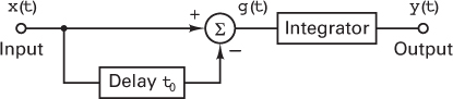
Figure P1.3
1.20. Given the spectrum
find the value of the signal bandwidth using the following bandwidth definitions:
Half-power bandwidth
Noise equivalent bandwidth
Null-to-null bandwidth
99% of power bandwidth (Hint: Use numerical methods.)
Bandwidth beyond which the attenuation is 35 dB
Absolute bandwidth
Questions
1.1. How does the plot of a signal’s autocorrelation function reveal its bandwidth occupancy? (See Section 1.5.4.)
1.2. What two requirements must be fulfilled in order to insure distortionless transmission through a linear system? (See Section 1.6.3.)
1.3. Define the parameter envelope delay or group delay. (See Section 1.6.3.)
1.4. What mathematical dilemma is the cause for there being several different definitions of bandwidth? (See Section 1.7.2.)