3
Image Quality
The performance assessment of image interpolation algorithms can be categorized into objective and subjective assessments, and they are just the two faces of the mirror. Since the interpolated images are to be perceived by human eyes, therefore, subjective analysis is considered to be the final quality assessment of the interpolated image. However, one's medicine is the other's poison. It is difficult if not impossible to provide a subjective analysis to the interpolated image as it requires time and money and is highly inconvenient. Not to mention that there is no commonly accepted subject quality measure or feature sets for all varieties of image interpolation problems. Researchers are devoting massive efforts in developing different objective quality assessment algorithms that take the human vision system (HVS) into consideration (to model and to approximate the behavior of human vision) such as to provide an objective mean to compare the visible artifacts generated throughout the interpolation process. These algorithms give objective quality score that mimic the subjective quality measure for the image under test, without going through the subjective quality analysis. The objective scores (which are sometimes referred to as index) of different quality assessment algorithms depend on how the visible artifacts are quantified and also the sources of the reference data for comparison. Therefore, it is important for the readers to understand the definition of visible artifacts in terms of their appearances and also the sources of the reference data, such that they can make appropriate choices of the objective quality assessment methods to be applied for their own purposes. In this chapter, we shall first introduce the different image features and also the image artifacts commonly observed in interpolated images in Section 3.1 , while the following will discuss the classification of quality assessment algorithms according to the sources of reference images.
The source of the reference image adopted in different quality assessment algorithms categorizes the algorithms into three groups, including full‐reference image quality index (FRIQ), no‐reference image quality index (NRIQ), and reduced‐reference image quality index (RRIQ). Among various image quality indices, the interest of this book is the FRIQ, because we have no difficulties to obtain the reference image in our analysis. The FRIQ scores the quality of the interpolated image by comparing it with a reference image, which is also known as the undistorted image. The algorithm makes use of certain parameters of the image to estimate the quality score of the interpolated image with reference to the undistorted image. A list of commonly applied FRIQ measures together with their analytic backgrounds will be discussed in Section 3.2 , in which all the algorithms focus on the some kinds of measures of the absolute difference in pixel intensities between the interpolated image and the reference image.
In Section 3.3 , we shall discuss a benchmark FRIQ, known as structural similarity (SSIM) index, which considers the HVS. The SSIM takes an in‐depth look on the impact of image structure on the assessment of image quality. The readers should note that neither subjective nor objective assessments could be used alone. It is always more convincing when both quality measures are applied together or at least applied a limited subjective quality measure to assist the objective assessment of the interpolated image quality.
3.1 Image Features and Artifacts
The human eye interprets the information in an image by classifying the image into different feature zones and determines the image quality by looking for visible artifacts, which refers to the features that should not exist in the particular feature zones. A rough classification of the different feature zones of a natural image can be illustrated by the natural image Cat in Figure 3.1 :
- 1. Homogeneous: The variations of the grayscales within these zones are small (or smaller than a predefined quantity), which makes interpolation artifacts (large pixel value variations) in these region to be easily detectable.
- 2. Textured: Regions with repetitive patterns and structures at various scales and orientations. The human eye is not very sensitive to pixel value variations within these zones, and thus interpolation artifacts are difficult to be detected in these regions.
- 3. Edges: The edges separate two homogeneous regions with different mean grayscales, which makes the interpolation artifacts in this zone readily noticeable.
Subjective quality assessment assesses the image quality through human eye, which is often considered to be the only “correct” way to evaluate the image quality. The subjective mean opinion score (MOS) is a popular method to achieve statistical significance. To achieve a satisfactory assessment result, which can be considered to be general and reliable, the number of participants should be as large as possible. As a result, each assessment will require an adequate number of participants, and a series of tests are required, making the experiment extremely time‐consuming and expensive. Therefore, a great deal of efforts has been made in recent years to develop objective image quality metrics that correlate with perceived quality measurement, which are the topics in Section 3.2 , where a number of FRIQ metrics will be discussed. Before we move onto FRIQ metrics, the following subsections will list the commonly observed visual artifacts in an interpolated image, so we could have a better understanding on the nature and origin of different image artifacts and how they are perceived by human eyes. In order to clearly display each image artifact, the synthetic image letter A, a noise‐free computer drawing with sharp edges will be used for illustration, instead of the natural image Cat (see Figure 3.2 ).
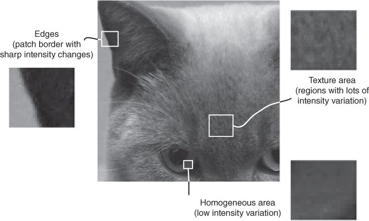
Figure 3.1 A natural image Cat showing three basic image features: homogeneous area, texture area, and edges.
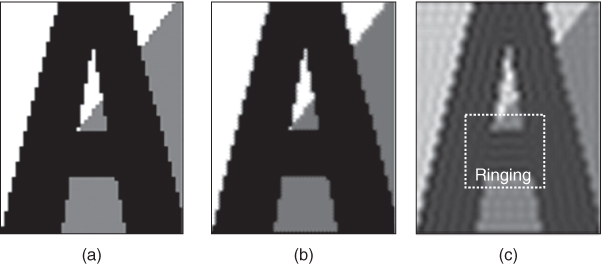
Figure 3.2 Image interpolation artifacts of the synthetic image letter A demonstrating (a) aliasing (jaggy), (b) blurring, and (c) edge halo and ringing.
3.1.1 Aliasing (Jaggy)
When the sampling frequency applied to generate the digital image is lower than the highest spatial frequency of the natural image under concern, sampling theorem (Section 1.1) tells us that the obtained digital image will be susceptible to aliasing noise. The aliasing distorted digital image is observed to have undesirable high frequency oscillation around the high spatial frequency region of the image. The aliasing noise is not only observed in the under‐sampled digital image but also observed in the interpolated image. This is because the frequency response of the interpolation kernel will almost likely not to be an ideal low‐pass filter, and hence the high frequency components of the aliasing component in the up‐sampling process will remain in the interpolated image. These high frequency noises will have the same effect in the interpolation process as that of the high frequency noises in the down‐sampling operation. An example of aliasing distorted image is shown in Figure 3.2 a, where the aliasing noise is observed as staircase‐like features and is therefore also known as “jaggy” artifact. This observation closely resembles the effect of aliasing noise in the down‐sampling process. Transitional pixels are required to smooth the sharp changes between the grayscales on the two sides of a sharp edge to make it to appear to be pleasant to human observation. Such transitional pixels occur naturally in images captured by digital camera. However, when such transitional pixels are lost in the down‐sampling process, they may not be reproduced in the interpolation process, thus generating an interpolated image corrupted by aliasing noise.
3.1.2 Smoothing (Blurring)
Smoothing or blurring is observed when the high frequency components are lost, which can happen in the texture‐rich regions or along/across edges. An example of “blurred” image is shown in Figure 3.2 b, where the letter A has a “washed‐out” appearance. In some cases, the smoothing is localized, thus producing undesirable piecewise constant or blocky regions in the interpolated image as shown in Figure 3.2 b. In particular, when the edges of the interpolated image are over‐smoothed, the interpolated image will appear to be out of focus, which can also be observed in Figure 3.2 b. While the smoothing problem can be the result of a number of operations, the most common cause is due to the application of an interpolation kernel that is low‐pass in nature. Such high frequency lossy interpolation process is vivid from the linear interpolation process of a sampled 1D step curve by linear interpolation as shown in Figure 3.3 , where the details will be discussed in Chapter . Figure 3.3 b shows the interpolation of a low‐resolution step function. The linear interpolation result obtained by averaging the two nearest‐neighbor pixels is shown in Figure 3.3 c, which shows the step is dispersed and becomes a ramp function when compared with the high‐resolution step function in Figure 3.3 a. We can easily conjecture from the linear interpolation process shown in Figure 3.3 that smoothing/blurring will occur in any interpolation process, which involves the estimation of unknown pixel by averaging the neighboring known pixels. The blurring problem worsens with increased interpolation kernel size, which will cause the averaging effect spans over a larger number of pixels.

Figure 3.3 Blurring effect of linear interpolation in one‐dimensional case: (a) original high‐resolution data points, (b) low‐resolution data obtained by subsampling, and (c) recovered data by linear interpolation.
3.1.3 Edge Halo
The edge halo can be considered as a visual artifact that is opposite to smoothing. An image corrupted with edge halo artifact is shown in Figure 3.2 c. It is vivid from Figure 3.2 c that the edges are observed to be over‐sharpened where white tracks are formed around the edges of the images, which creates an impression of an additional false edge and hence its name “halo.” The halo is more apparent than the contrast between the two sides of the edges, which creates the illusion of enhanced sharpness. But edge halos are undesirable in natural image interpolation, especially in the case where it creates ghost images around natural objects.
3.1.4 Ringing
Besides the artifacts caused by nonideal frequency response of the interpolation kernel, the visual quality of the interpolated image is also affected by the spatial properties of the interpolation kernel. Ringing or oscillating wavelike artifacts can be observed in the interpolated image because most good interpolation kernels are functions of oscillating waves (see Figure 3.2 c). The extent of the ringing artifact is proportional to the length of the interpolation kernel. Furthermore, ringing often happens around step edges, where the oscillating waves are the natural results of the Gibbs phenomenon (both intensity and spatial occupancy) [43 ]. Note that the discontinuity at the image block edges is also considered to be a kind of step edges and hence will cause ringing noise too. An appropriate interpolation kernel (smooth and non‐oscillating spatial function) or high sampling rate can help to reduce the ringing artifacts.
3.1.5 Blocking
Besides the aforementioned artifacts, there is another artifact known as blocking artifact (also known as “zigzag”), which has a similar outlook as that of jaggies, where there are discontinuities within or along the image features. However, the discontinuity looks more like that of a repetitive block of image feature copied from nearby regions, and this kind of artifacts is also known as the blocking effect. Moreover, the origin of the blocking artifact, in the frequency response aspect, is different from that forming the jaggy artifacts. The blocking artifact is strengthened by the finite kernel size in spatial domain interpolation where the size of the kernel is smaller than the entire feature size. It can also be caused by cropping the high frequency components of the image due to finite block size of signal processing tool (also known as the kernel size). It becomes severe when the interpolation magnifies the image for several times. More details will be discussed in Chapter 5.
3.2 Objective Quality Measure
Objective quality measures are the alternative ways to assess the interpolated image quality other than the subjective quality measures. They provide automatic evaluation through quantifying metrics known as the objective image quality metrics. Unlike subjective quality measure, which has to be performed as a blind quality assessment for fair comparison, objective quality measure could be performed without human interaction, and the output of such assessment is almost identical (the variations are the results of accuracy of the computing system and any variations induced are systematic and consistent for all test images). As discussed in the introduction of this chapter, objective quality measures can be classified into three groups depending on how much the original (high resolution) image information is available. In this book, we shall only focus on the FRIQ.
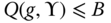
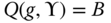
The FRIQ metric ![]() correlates the perceived difference (quality) between the interpolated image
correlates the perceived difference (quality) between the interpolated image ![]() and the high‐resolution reference image
and the high‐resolution reference image ![]() , which also satisfies the following conditions:
, which also satisfies the following conditions:
- 1. Symmetric:
 .
. - 2. Boundedness:
 for a constant
  .
. - 3. Unique maximum:
 if and only if
  (no distortion between the two images).
Among various FRIQ metrics, the mean squares error (MSE) and the peak signal‐to‐noise ratio (PSNR) are two commonly used metrics. These metrics are convenient in their simplicity to compute, and their physical meanings as similarity measurement metrics by comparing the intensity of the two images in a pixel‐by‐pixel fashion, where neither the structure of the image nor human perception to the image features is considered. Therefore, they may not match well with the subjective quality measure and may lead to undesirable results in some cases.
To improve the assessment accuracy, the similarity measures have to be modified to make it compatible with the HVS. Edge peak signal‐to‐noise ratio (EPSNR) discussed in Section 3.2.3 is a modified PSNR, which considers the image edges by applying different weighting factors onto the edge and non‐edge pixels. EPSNR can be considered as our first step to perform objective similarity measure in response to the HVS. A more sophisticated and widely applied HVS modified similarity measures, the SSIM [63 ], will be presented in Section 3.3 .
Once an objective quality metric is chosen, it can be applied to evaluate the performance of an image interpolation algorithm through a scheme as shown in Figure 3.4 . This scheme considers a high‐resolution reference image, which is first down‐sampled by a factor of two horizontally and vertically and then interpolated back to its original image size by the interpolation algorithm under test. The difference between the original high‐resolution image and the interpolated image is compared by means of the chosen FRIQ metric. It should be noted that the degree of degradation of the interpolated image is content‐dependent. Therefore, it is a common practice to evaluate the image interpolation method using multiple reference images that have different image details and cover a wide class of image features that are important for the applications with the applied image interpolation algorithm under concern. For simplicity, and clarity of discussions in this book, we shall concentrate on the case of using the Cat and letter A as reference images.
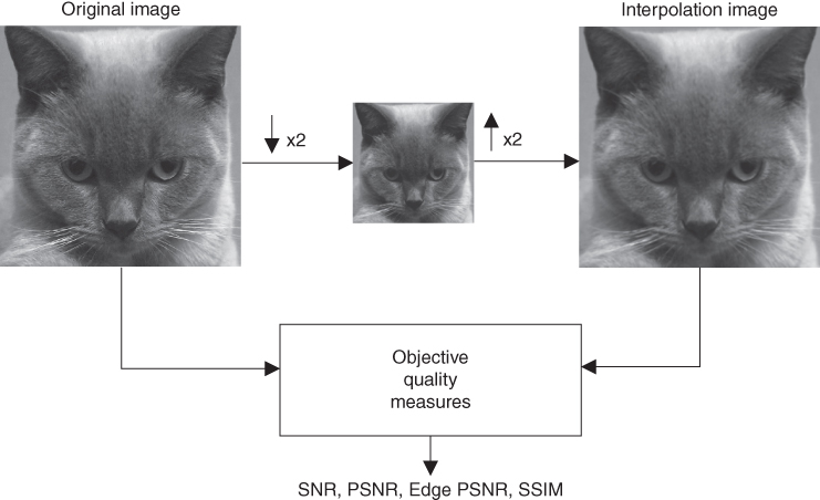
Figure 3.4 Image interpolation quality computation.
3.2.1 Mean Squares Error
Intuitively, the interpolated image can be regarded as the sum of the high‐resolution reference image and an error signal (also known as error image). Therefore, the MSE is one of the most traditional similarity measures. Starting with the computation of the error image ![]() (also known as the difference image) between the interpolated image array
(also known as the difference image) between the interpolated image array ![]() and the high‐resolution reference image array
and the high‐resolution reference image array ![]() , both of size
, both of size ![]() by
by
The MATLAB source code in MATLAB 3.2.1 implements the function to compute the error image.

With the availability of the error image, the total error between the two images is given by ![]() . However, the elements in
. However, the elements in ![]() have both positive and negative values. Therefore, it is more reasonable to consider the magnitude of
have both positive and negative values. Therefore, it is more reasonable to consider the magnitude of ![]() . The
mean absolute error
(MAE) (also known as mean absolute difference) provides such a quality factor between the interpolated image array
. The
mean absolute error
(MAE) (also known as mean absolute difference) provides such a quality factor between the interpolated image array ![]() and the high‐resolution reference image array
and the high‐resolution reference image array ![]() , both of size
, both of size ![]() .
.

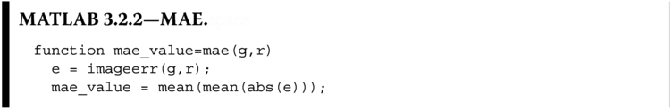
The MATLAB source code in MATLAB 3.2.2 implements the function to compute the error image.
In particular, the most popular quality factor is the MSE, which is equivalent to the computation of the square power of the error signal ![]() . The MSE is defined as
. The MSE is defined as

The MATLAB source code listed in MATLAB 3.2.3 implements the MSE function.

It is also common to give the MSE, mse_value, through the square root operation to generate a value that resembles the meaning of average pixel error of the two images, which is known as the
root mean squares error
(RMSE).
The MATLAB source code listed in MATLAB 3.2.4 computes the RMSE by means of the function mse.

It should be noted that g and r should have the same array size to avoid runtime error.
3.2.2 Peak Signal‐to‐Noise Ratio
The MSE does not consider the dynamic range of the image but only the absolute error in between two images and is therefore biased. Such bias can be removed by normalization. The PSNR is the most commonly used normalized objective quality metric for interpolated image quality assessment. The denominator of the PSNR is the MSE, while the numerator is the highest dynamic range achievable by the image function under consideration, which is also known as the ratio between the maximal power of the reference image and the noise power of interpolated image. It is represented in the logarithmic domain in decibels (dB) because the powers of signals usually have a wide dynamic range. An example for PSNR computed for an ![]() ‐bit grayscale image is given by
‐bit grayscale image is given by
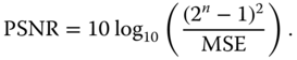
For example, an 8‐bit/pixel grayscale image will have ![]() as the numerator of the PSNR. The MATLAB code 3.2.5 will compute the PSNR with the assumption that the input image array in “
as the numerator of the PSNR. The MATLAB code 3.2.5 will compute the PSNR with the assumption that the input image array in “uint8” datatype and thus ![]() .
.

The above discussed quality metrics can be easily extended to color images by treating each color channel independently as a grayscale image. In the case of color images in RGB domain, the PSNR of the three color channels are first computed and then recombined to give the final PSNR by averaging as
where ![]() ,
, ![]() , and
, and ![]() are the PSNR values for the red, green, and blue channels of the color image computed with Eq. (3.5 ), respectively. Without loss of generality, the rest of the book will use PSNR to imply both the PSNR in Eq. ( 3.5
) for grayscale images and
are the PSNR values for the red, green, and blue channels of the color image computed with Eq. (3.5 ), respectively. Without loss of generality, the rest of the book will use PSNR to imply both the PSNR in Eq. ( 3.5
) for grayscale images and ![]() in Eq. (3.6 ) for color images depending on the context.
in Eq. (3.6 ) for color images depending on the context.
The PSNR is widely used because it is simple to calculate, has clear physical meanings, and is mathematically easy to deal with for optimization purposes. High PSNR value of the interpolated image is more favorable because it implies less distortion. However, the PSNR measure is not ideal. Its main shortcoming is that the signal strength is estimated by the highest dynamic range of the image that can be possibly achieved, which is ![]() , rather than the actual signal strength of the image. Furthermore, PSNR does not take the HVS into consideration. It has been widely criticized for not correlating well with subjective quality measurement. One of such quality is the preservation of edges in the interpolated image. Otherwise, the PSNR is considered to be able to provide an acceptable measure for comparing interpolation results.
, rather than the actual signal strength of the image. Furthermore, PSNR does not take the HVS into consideration. It has been widely criticized for not correlating well with subjective quality measurement. One of such quality is the preservation of edges in the interpolated image. Otherwise, the PSNR is considered to be able to provide an acceptable measure for comparing interpolation results.
3.2.3 Edge PSNR
A critical shortcoming of MSE and PSNR is that they are not compliant to HVS. This problem is vivid in the interpolated images in Figure 3.5 . In this example, the down‐sampled Cat image is interpolated by two different algorithms to produce (a) and (b). It is vivid that the image (a) has better visual quality, while (b) is visually observed to be seriously degraded; however, the PSNR of the image in (a) and (b) are both close to 23.04 dB. This is because the HVS perceives pixels differently and depends on their visual features, while PSNR considers all pixels to be the same. As a result, although being an objective and simple measure, the PSNR might lead to a totally wrong quality measurement result.
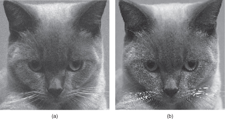
Figure 3.5 The Cat image is down‐sampled by a scaling factor of 2 and then restored to its original size by the same scaling factor by different algorithms to produce (a) and (b) with the PSNR of both images close to 23.04 dB.
A simple step to improve the correlation between PSNR and visual quality of the interpolated image is to incorporate the differentiation of pixels perceived by the HVS. This can be achieved by assigning different weights to the edge and non‐edge pixels in the error image when computing the PSNR to simulate the relative importance of different pixels perceived by the HVS. The edge pixels can be located by the edge extraction algorithm presented in Section 2.5. It should be noted that applying different edge detection algorithms will lead to minor differences in the result. The Sobel edge detector is being adopted by the International Telecommunication Union (ITU) [1 ] for the EPSNR. Without loss of generality, assume the weight ![]() is assigned to the edge pixels and
is assigned to the edge pixels and ![]() to the non‐edge pixels. The error image should be modified as
to the non‐edge pixels. The error image should be modified as
where ![]() is the edge map of the interpolated image with 0 being the value assigned to edge pixels and 1 be assigned to non‐edge pixels.
is the edge map of the interpolated image with 0 being the value assigned to edge pixels and 1 be assigned to non‐edge pixels.
Besides the consideration of the HVS sensitivity differences toward edge and non‐edge pixels in the interpolated image, the actual contrast of the interpolated image should also be addressed by applying the peak intensity pixel value in the computation of the objective metric instead of the highest possible pixel value as in Eq. ( 3.5 ). The MATLAB source code 3.2.6 computes the EPSNR.

where edge is a MATLAB built‐in function that returns the binary edge map of the input image. The Sobel filter and the sensitivity threshold t have been chosen as the input parameters for edge in Listing 3.2.6. The matrix eedge is the error image ![]() . As you may have noticed from the MATLAB function
. As you may have noticed from the MATLAB function epsnr, the mean squares edge error is normalized not by the image size, but by the number of pixels that are declared as edge pixels in ![]() . Similar to PSNR, the higher the EPSNR, the less the distortion will be observed on the image edges, and thus the better in perceived image quality. Finally, it must be pointed out that the EPSNR result is deeply affected by the threshold
. Similar to PSNR, the higher the EPSNR, the less the distortion will be observed on the image edges, and thus the better in perceived image quality. Finally, it must be pointed out that the EPSNR result is deeply affected by the threshold t, which is the threshold value applied to the gradient results obtained by the Sobel filter to decide each pixel locations to be edge or non‐edge pixels. The threshold value should be determined by the local contrast of the image, and therefore, a global threshold might not produce good edge detection results as discussed in Section 2.5 and hence biased the EPSNR. The following will discuss the structure similarity metric that applies localized analysis to evaluate the difference between the two images.
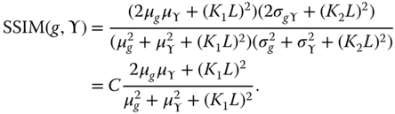
3.3 Structural Similarity
The EPSNR is a good start to apply HVS to objective quality measure, but it will suffer from several problems. First, it is a point‐wise measure. Although the edge map is generated with Sobel filter, which has a detector kernel size larger than a single pixel, the actual computation of the error image is still a point‐wise routine. Knowing the luminance and contrast of the image observed by HVS is not a point‐wise process, but through a small localized region. Therefore, it will be critical to convert the point‐wise operation to a localized small image region in the objective quality metric. Second, the point‐wise operation of EPSNR is basically a luminance comparison operation. The contrast and the structure of the localized image region are being ignored in the computation of EPSNR.
To render the perception of luminance, contrast, and structure by human vision in the quality measurement, a variety of HVS compatible objective quality metrics are proposed for interpolation image quality evaluation [26, 64 ]. Among those reported metrics, the SSIM index proposed by Wang et al. [63 ] is a benchmark metric in literature, which correlates well with the perceptual image quality. The SSIM is obtained as the product of the luminance, contrast, and structural factors between the interpolated image (![]() ) and the reference image (
) and the reference image (![]() ). These factors are obtained with the use of basic statistical parameters like mean, variance, and covariance as
). These factors are obtained with the use of basic statistical parameters like mean, variance, and covariance as

where ![]() and
and ![]() are added to provide stability to each factors, such as to prevent the denominator becoming zero and at the same time bounding the metric to be within a predetermined range (in the case of Eq. (3.8 ), the fraction will be in the range of
are added to provide stability to each factors, such as to prevent the denominator becoming zero and at the same time bounding the metric to be within a predetermined range (in the case of Eq. (3.8 ), the fraction will be in the range of ![]() but not equal to 0), and
but not equal to 0), and ![]() and
and ![]() are the mean and variance of the random variable
are the mean and variance of the random variable ![]() , respectively. Note that the statistical features are computed locally in Eq. ( 3.8
). However, the images are generally nonstationary with space‐variant image structures, as shown in Section 3.1 . Therefore, the localized regions applied to compute Eq. ( 3.8
) are extracted by sliding window
, respectively. Note that the statistical features are computed locally in Eq. ( 3.8
). However, the images are generally nonstationary with space‐variant image structures, as shown in Section 3.1 . Therefore, the localized regions applied to compute Eq. ( 3.8
) are extracted by sliding window ![]() to adapt to the space‐variant image structure. Starting from the top‐left corner of the image, a sliding window of size
to adapt to the space‐variant image structure. Starting from the top‐left corner of the image, a sliding window of size ![]() moves pixel by pixel horizontally and vertically through all the rows and columns of the image until the bottom‐right corner is reached. At the
moves pixel by pixel horizontally and vertically through all the rows and columns of the image until the bottom‐right corner is reached. At the ![]() th step, the local quality index
th step, the local quality index ![]() is computed within the sliding window. As a result, each processed window will assign an SSIM value at the corresponding pixel coordinate located at the center of the processing window. This forms an SSIM map of the SSIM value for each pixel of the interpolated image under concern. If there are a total of
is computed within the sliding window. As a result, each processed window will assign an SSIM value at the corresponding pixel coordinate located at the center of the processing window. This forms an SSIM map of the SSIM value for each pixel of the interpolated image under concern. If there are a total of ![]() steps, then the overall quality index
steps, then the overall quality index ![]() is the mean SSIM (MSSIM) given by averaging all the results obtained in the
is the mean SSIM (MSSIM) given by averaging all the results obtained in the ![]() steps.
steps.

It is vivid that the dynamic range of both SSIM and MSSIM are ![]() . The best value 1 can be achieved if and only if
. The best value 1 can be achieved if and only if ![]() for every pixel. The lowest value
for every pixel. The lowest value ![]() occurs when
occurs when ![]() for every pixel. The following subsections will discuss the mathematical formulation of SSIM in Eq. ( 3.8
) in terms of the three HVS components, namely, the luminance, contrast, and structural components.
for every pixel. The following subsections will discuss the mathematical formulation of SSIM in Eq. ( 3.8
) in terms of the three HVS components, namely, the luminance, contrast, and structural components.
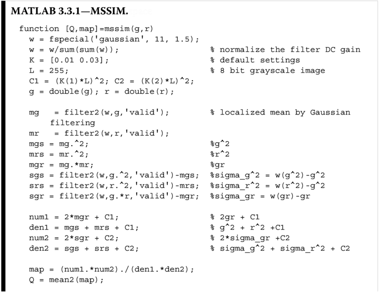
The MATLAB Listing 3.3.1 implements Eq. ( 3.8
) with the sliding window of a ![]() Gaussian window with unit gain and
Gaussian window with unit gain and ![]() ,
, ![]() , and
, and ![]() , where
, where ![]() is the dynamic range of the pixel intensity for an 8‐bit grayscale image. The Gaussian window is chosen instead of other window functions because it can avoid blocking effect, which is predominant in windowed local spatial analysis. To understand how
is the dynamic range of the pixel intensity for an 8‐bit grayscale image. The Gaussian window is chosen instead of other window functions because it can avoid blocking effect, which is predominant in windowed local spatial analysis. To understand how mssim works, let us rewrite SSIM in Eq. ( 3.8
) as
where
The denominators ![]() and
and ![]() are given by
are given by
From Eqs. (3.11 ) to (3.14 ), MATLAB Listing 3.3.1 implements them equation by equation. In particular, the implementation chooses ![]() and
and ![]() , which is also the particular choice in [63 ]. Note that the mean values of all the small localized blocks (for
, which is also the particular choice in [63 ]. Note that the mean values of all the small localized blocks (for mg, mr, sgs, srs, and sgr) are implemented with Gaussian smoothing, which captures the nonstationarity of the image structure in the localized regions.
To investigate the effect of ![]() and
and ![]() , let us consider an original image and its distorted version by additive Gaussian noise (
, let us consider an original image and its distorted version by additive Gaussian noise (![]() and
and ![]() ) as shown in Figure 3.5 a. The calculated MSSIM for these two images under different
) as shown in Figure 3.5 a. The calculated MSSIM for these two images under different ![]() and
and ![]() are tabulated in Table 3.1 . The percentage difference of the MSSIM for
are tabulated in Table 3.1 . The percentage difference of the MSSIM for ![]() and
and ![]() is almost
is almost ![]() and for values
and for values ![]() and
and ![]() is almost
is almost ![]() compared with the nominal MSSIM value computed with
compared with the nominal MSSIM value computed with ![]() and
and ![]() . These errors in estimation of the quality of the image can lead to faulty decisions, and we shall discuss the effect of these two parameters in terms of luminance, contrast, and structure in the following sections.
. These errors in estimation of the quality of the image can lead to faulty decisions, and we shall discuss the effect of these two parameters in terms of luminance, contrast, and structure in the following sections.
Table 3.1 MSSIM value of Figure 3.5 a with different ![]() and
and ![]() values.
values.
|
|
|
SSIM |
| 0.01 | 0.03 | 0.4184 |
| 0.05 | 0.05 | 0.5259 |
| 0.01 | 0.01 | 0.3411 |
3.3.1 Luminance
The mean luminance ![]() can be used to compare the luminance of two images. A simple comparison metric can be formed by considering the ratio between the geometric means and the arithmetic means of the two luminance means as
can be used to compare the luminance of two images. A simple comparison metric can be formed by considering the ratio between the geometric means and the arithmetic means of the two luminance means as

such that ![]() and equals to 1 if and only if
and equals to 1 if and only if ![]() . The factor
. The factor ![]() is added to the computation of
is added to the computation of ![]() to ensure the robustness of
to ensure the robustness of ![]() . Otherwise, with
. Otherwise, with ![]() and both
and both ![]() , the metric will be undefined with
, the metric will be undefined with ![]() . Among all the possible
. Among all the possible ![]() values, SSIM selected
values, SSIM selected
where ![]() is the dynamic range of the pixel intensity. In an 8‐bit grayscale image,
is the dynamic range of the pixel intensity. In an 8‐bit grayscale image, ![]() and the squares are the result of considering a two‐dimensional image. As a result,
and the squares are the result of considering a two‐dimensional image. As a result, ![]() is totally controlled by
is totally controlled by ![]() and should be chosen to avoid the luminance component to dominate SSIM.
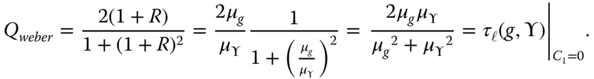
and should be chosen to avoid the luminance component to dominate SSIM. ![]() has been suggested in [63 ], which has shown to provide a useful SSIM metric. Incidentally, this definition is also compatible with the Weber's law of just‐noticeable luminance change, which states that the just‐noticeable luminance change within a local area in an image depends on the relative change
has been suggested in [63 ], which has shown to provide a useful SSIM metric. Incidentally, this definition is also compatible with the Weber's law of just‐noticeable luminance change, which states that the just‐noticeable luminance change within a local area in an image depends on the relative change ![]() in mean luminance with the localized area under concern with
in mean luminance with the localized area under concern with ![]() . The equivalent between Weber's luminance quality index and
. The equivalent between Weber's luminance quality index and ![]() can be established by
can be established by
To incorporate the local statistical property of the nonstationary image signal into the metric, a window function is applied to preprocess a localized image block. The applied window function has to have unit gain and be circular symmetric to avoid spatial bias. One of such windows is the Gaussian window. In this book, a Gaussian window of size ![]() with standard deviation of 1.5 will be applied to preprocess the image signal. The mean
with standard deviation of 1.5 will be applied to preprocess the image signal. The mean ![]() of the image block
of the image block ![]() will be replaced with the Gaussian weighted mean, which can be conveniently implemented by convolution operation as
will be replaced with the Gaussian weighted mean, which can be conveniently implemented by convolution operation as
In MATLAB, this can be implemented with the filter2 operation as
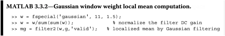
which is implemented in MATLAB Listing 3.3.1 to generate a map of localized mean weighted by a Gaussian window.
3.3.2 Contrast
The contrast component in SSIM is computed in a similar manner as that of the luminance component with ![]() being replaced by
being replaced by ![]() as
as
such that ![]() and it equals to 1 if and only if
and it equals to 1 if and only if ![]() . The factor
. The factor ![]() has a similar function as that of
has a similar function as that of ![]() , and thus it is also chosen to be equal to
, and thus it is also chosen to be equal to
Similar to ![]() ,
, ![]() is totally controlled by
is totally controlled by ![]() and should be chosen to avoid the luminance component to dominate the SSIM.
and should be chosen to avoid the luminance component to dominate the SSIM. ![]() has been suggested in [63 ], which has shown to provide useful SSIM metric for interpolation algorithm performance comparison. Eq. (3.19 ) has shown that the metric
has been suggested in [63 ], which has shown to provide useful SSIM metric for interpolation algorithm performance comparison. Eq. (3.19 ) has shown that the metric ![]() depends on the relative contrast changes, which is consistent with the contrast masking property of the HVS.
depends on the relative contrast changes, which is consistent with the contrast masking property of the HVS.
3.3.3 Structural
The structural similarity between two random variables is best investigated by the Pearson correlation [35 ], and thus the structure component in SSIM is given by

such that ![]() . If we discard
. If we discard ![]() , the Pearson correlation factor
, the Pearson correlation factor ![]() when the two images
when the two images ![]() and
and ![]() are not related. If the two images are associated with each other,
are not related. If the two images are associated with each other, ![]() . In particular
. In particular ![]() when
when ![]() and
and ![]() can form a linear relationship,
can form a linear relationship, ![]() with constants
with constants ![]() and
and ![]() . This relationship implies that the two images are an exact copy of each other structurally with difference in lighting condition only. The factor
. This relationship implies that the two images are an exact copy of each other structurally with difference in lighting condition only. The factor ![]() is similar to
is similar to ![]() and
and ![]() . The overall SSIM is given by the product of these three metrics,
. The overall SSIM is given by the product of these three metrics, ![]()
![]() , and
, and ![]() as
as
It is vivid from Eqs. ( 3.19
) and (3.21 ) that the numerator of ![]() and the denominator of
and the denominator of ![]() share the same factor except the constants
share the same factor except the constants ![]() and
and ![]() . Therefore, there are two factors that can be eliminated from SSIM. Furthermore,
. Therefore, there are two factors that can be eliminated from SSIM. Furthermore, ![]() and
and ![]() are unified to form a single constant and hence obtained the SSIM in Eq. ( 3.8
).
are unified to form a single constant and hence obtained the SSIM in Eq. ( 3.8
).
Readers should also take note that when ![]() and
and ![]() are both equal to zero, the metric will be the same as the
universal quality index
(UQI).
are both equal to zero, the metric will be the same as the
universal quality index
(UQI).
3.3.4 Sensitivity of SSIM
In the above sections, we have discussed how the luminance, contrast, and structure of an image are considered in the SSIM. Eq. ( 3.8
) tells us that SSIM is a function of image parameters (![]() ,
, ![]() ,
, ![]() ,
, ![]() , and
, and ![]() ) and user‐defined functions (
) and user‐defined functions (![]() and
and ![]() ). These two user‐defined functions adjust the impact of luminance, contrast, and structure of a natural image toward the SSIM computation. The values of
). These two user‐defined functions adjust the impact of luminance, contrast, and structure of a natural image toward the SSIM computation. The values of ![]() and
and ![]() are controlled by two user input parameters,
are controlled by two user input parameters, ![]() and
and ![]() , respectively. In the following sections, we shall explore the sensitivity of SSIM toward the parameters
, respectively. In the following sections, we shall explore the sensitivity of SSIM toward the parameters ![]() and
and ![]() (
(![]() and
and ![]() ) and find out the appropriate range of
) and find out the appropriate range of ![]() and
and ![]() that should be chosen such that a fair SSIM index could be generated that provides meaningful comparison among wide range of natural images.
that should be chosen such that a fair SSIM index could be generated that provides meaningful comparison among wide range of natural images.
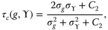
3.3.4.1  Sensitivity
To understand the sensitivity of SSIM toward ![]() , a sensitivity analysis can be performed by rewriting the SSIM function as depicted in Eq. ( 3.8
) as
, a sensitivity analysis can be performed by rewriting the SSIM function as depicted in Eq. ( 3.8
) as
The sensitivity of SSIM toward ![]() is the first derivative of Eq. (3.6 ) with respect to
is the first derivative of Eq. (3.6 ) with respect to ![]() with
with ![]() ,
, ![]() ,
, ![]() ,
, ![]() ,
, ![]() , and
, and ![]() considered to be constant, such that we have
considered to be constant, such that we have

with ![]() , and
, and ![]() . It is vivid that the sensitivity of SSIM toward
. It is vivid that the sensitivity of SSIM toward ![]() depends on
depends on ![]() ,
, ![]() , and
, and ![]() , but to what extent?
, but to what extent?

Figure 3.6
The sensitivity of SSIM toward  with varying
  at different
  (the solid lines) and the sensitivity of SSIM toward
  with varying
  at different
  (the dashed lines). (See insert for color representation of this figure.)
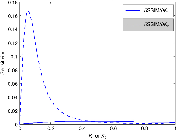
Figure 3.7
The sensitivity of SSIM toward  with varying
  (solid lines) and the sensitivity of SSIM toward
  with varying
  (dashed lines).
It should be noted that for a given image, ![]() has to be a constant depending on the data type of the image. For example, an image in
has to be a constant depending on the data type of the image. For example, an image in uint8, ![]() . To simplify and without affecting the discussions, we generalize to use
. To simplify and without affecting the discussions, we generalize to use ![]() to represent
to represent ![]() and
and ![]() , unless otherwise specified. With
, unless otherwise specified. With ![]() being the mean intensity of an image, it is vivid that the dynamic range of
being the mean intensity of an image, it is vivid that the dynamic range of ![]() is 0–255. In other words, no matter which interpolation method has been applied to the interpolated image,
is 0–255. In other words, no matter which interpolation method has been applied to the interpolated image, ![]() . To focus our study to the impact of the choice of
. To focus our study to the impact of the choice of ![]() toward the SSIM sensitivity to
toward the SSIM sensitivity to ![]() , we consider
, we consider ![]() ,
, ![]() , and
, and ![]() , and the SSIM sensitivity to
, and the SSIM sensitivity to ![]() as a function of
as a function of ![]() at
at ![]() , 0.03, and 0.05 are plotted in Figure 3.6 (solid lines). It should be noted that it is rare in natural image to have
, 0.03, and 0.05 are plotted in Figure 3.6 (solid lines). It should be noted that it is rare in natural image to have ![]() equal 0 or 255, as
equal 0 or 255, as ![]() implies that all pixels within the localized image block to be 0, while
implies that all pixels within the localized image block to be 0, while ![]() implies all pixels within the localized image block to be 255. It is because there is always a background noise generated from the capture device, and hence a large region of pure color seldom happens in the captured images. Therefore, we can ignore the part of the SSIM sensitivity to
implies all pixels within the localized image block to be 255. It is because there is always a background noise generated from the capture device, and hence a large region of pure color seldom happens in the captured images. Therefore, we can ignore the part of the SSIM sensitivity to ![]() curves at the two ends. In this case, the remaining curves are all fairly flat and close to zero, which allows us to conclude that the SSIM sensitivity to
curves at the two ends. In this case, the remaining curves are all fairly flat and close to zero, which allows us to conclude that the SSIM sensitivity to ![]() is independent to the choice
is independent to the choice ![]() . We can further conclude that the SSIM of a natural image is insensitive to
. We can further conclude that the SSIM of a natural image is insensitive to ![]() for a fixed
for a fixed ![]() . Figure 3.7 shows the sensitivity of SSIM as a function of
. Figure 3.7 shows the sensitivity of SSIM as a function of ![]() (see the solid line), where the curve is obtained by considering
(see the solid line), where the curve is obtained by considering ![]() and
and ![]() to be 10
to be 10![]() greater than
greater than ![]() and
and ![]() , respectively. The curve is almost independent to
, respectively. The curve is almost independent to ![]() , which further confirms the above conjecture.
, which further confirms the above conjecture.
3.3.4.2  Sensitivity
Similar to Section 3.3.4.1 , the sensitivity of SSIM toward ![]() can be analyzed by rewriting Eq. ( 3.8
) as
can be analyzed by rewriting Eq. ( 3.8
) as

The sensitivity of SSIM to ![]() is the first derivative of SSIM with respect to
is the first derivative of SSIM with respect to ![]() and is given by
and is given by
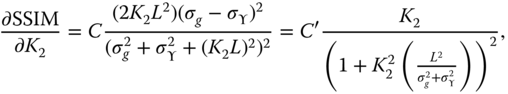
with ![]() and
and ![]() . It is vivid from Eq. (3.26 ) that the sensitivity of SSIM toward
. It is vivid from Eq. (3.26 ) that the sensitivity of SSIM toward ![]() depends on
depends on ![]() ,
, ![]() , and
, and ![]() . To simplify and without affecting the discussions, we decided to use
. To simplify and without affecting the discussions, we decided to use ![]() to represent
to represent ![]() and
and ![]() , unless otherwise specified. To focus our study to the impact of the choice of
, unless otherwise specified. To focus our study to the impact of the choice of ![]() toward the SSIM sensitivity to
toward the SSIM sensitivity to ![]() , we consider
, we consider ![]() ,
, ![]() , and
, and ![]() . The SSIM sensitivity to
. The SSIM sensitivity to ![]() as a function of
as a function of ![]() at
at ![]() , 0.03, and 0.05 is plotted in Figure 3.6 (dashed lines) with
, 0.03, and 0.05 is plotted in Figure 3.6 (dashed lines) with ![]() . It is vivid from Figure 3.6 that the SSIM sensitivity to
. It is vivid from Figure 3.6 that the SSIM sensitivity to ![]() with respect to
with respect to ![]() is sensitive to
is sensitive to ![]() . The
. The ![]() is more sensitive to
is more sensitive to ![]() when
when ![]() is small (less than
is small (less than ![]() ). It can also observe from Figure 3.6 that the sensitivity increases with large
). It can also observe from Figure 3.6 that the sensitivity increases with large ![]() . Figure 3.7 shows the sensitivity of SSIM toward
. Figure 3.7 shows the sensitivity of SSIM toward ![]() as a function of
as a function of ![]() (see the dashed line), where the curve is obtained by considering
(see the dashed line), where the curve is obtained by considering ![]() and
and ![]() to be 10
to be 10![]() greater than
greater than ![]() and
and ![]() , respectively. Both
, respectively. Both ![]() and
and ![]() have chosen to be below 15, such that
have chosen to be below 15, such that ![]() is the most sensitive with respect to
is the most sensitive with respect to ![]() , but the curve in Figure 3.7 exhibits a much less magnitude when compared with that shown in Figure 3.6 . It shows that
, but the curve in Figure 3.7 exhibits a much less magnitude when compared with that shown in Figure 3.6 . It shows that ![]() is also not sensitive to the variation in
is also not sensitive to the variation in ![]() . In conclusion, it is more appropriate to choose both
. In conclusion, it is more appropriate to choose both ![]() and
and ![]() to be small such that both the sensitivity of
to be small such that both the sensitivity of ![]() and
and ![]() are kept to minimal. Therefore, Wang et al. [63] proposed to use
are kept to minimal. Therefore, Wang et al. [63] proposed to use ![]() and
and ![]() in the SSIM analysis, which is generally suitable for wide range of natural images.
in the SSIM analysis, which is generally suitable for wide range of natural images.
3.4 Summary
In this chapter, we have introduced the idea of image quality measurement, which computes the performance of an interpolation algorithm. In our discussions, we have particularly chose full‐reference quality measurement, where the original (distortion free) high‐resolution image is considered to be available prior to comparison. Both objective and subjective image quality measurements have been discussed. The objective quality measurement, in contrast to the subjective measurement, is conducted by the image quality metric that counts the difference between the original image and the distorted image. MSE is the most common objective quality measurement metrics that is widely used in literature, and it forms the basis of other objective quality metrics, such as the PSNR and EPSNR. Objective quality measure plays an important role in a variety of image interpolation applications. Firstly, it can dynamically control and adjust image quality in real time. Secondly, it can be used to optimize algorithms and parametric settings of image interpolation systems. Thirdly, it can be used to benchmark image interpolation systems.
However, human vision perceives and interprets different image features differently, and the distortion on the image contents perceived by different people may be different. It is difficult if not impossible to quantify such subject perception because it will require a large amount of data collected from a large number of interviewees to generate fair comparison results, which is very complicated and time‐consuming. A series of image quality metrics have been developed to model the HVS in the perception of different image features and image structures, which form tools to quantify the subjective measures in a general way, and without any tedious data collection process. In this chapter, a benchmark subjective measurement known as SSIM has been chosen to illustrate the idea of subjective quality measurement. SSIM considers the image distortion through three aspects: luminance variation, contrast variation, and image structure variation. These three image features are the most sensitive information that the human visual system would consider. To analyze the generality of the SSIM, its sensitivity toward image contents, through varying the intensity means (![]() ), intensity variances (
), intensity variances (![]() ), and user‐defined parameters (
), and user‐defined parameters (![]() and
and ![]() ),is discussed. Although SSIM is generally image dependent, with a particular range of
),is discussed. Although SSIM is generally image dependent, with a particular range of ![]() to
to ![]() (in our case, we set
(in our case, we set ![]() and
and ![]() ), the results will be valid for a wide range of natural images. The reasons behind the performance robustness of SSIM are discussed by considering the sensitivity analysis of SSIM toward the variation of
), the results will be valid for a wide range of natural images. The reasons behind the performance robustness of SSIM are discussed by considering the sensitivity analysis of SSIM toward the variation of ![]() and
and ![]() .
.
The MATLAB implementations of the objective and subjective quality measurements are listed for the readers to understand and to provide practical implementations of our discussions and applications in later chapters.
3.5 Exercises
- 3.1
Modify the MATLAB function
msesuch that it will verify the size of the input images matrices to have the same size. Otherwise, it will output an error message ofimages are not the same sizeand setmse=NaN. - 3.2 Besides the image interpolation quality computation method shown in Figure 3.4 , it has been proposed in literature that the objective quality measures can be obtained by computing the quality metrics between the original image and an image obtained by:
- First interpolating the original image and then down‐sample it back to the original image size.
- Twelve successive rotation of
 of the original image.
Please comment on the applicability of the above quality metric evaluation methods.
- 3.3 Down‐sample the Cat image by
directdsin Section 2.7.2.1 to generatef. Interpolate the down‐sampled Cat image by bilinear interpolation method using MATLAB built‐in functioninterp2(f,2).- Compute the error image
eof the interpolated imagefand the original image. Rescale the error image to make it span the numerical range of [0, 255]. Plot the scaled error image. - Compute the SSIM of
fwith the default and
and  used in Section 3.3 . Rescale the SSIM map to span the numerical range of [0, 255]. Plot the scaled SSIM map.
 - Compute the edge image of
fof the interpolated image using MATLAB built‐in Sobel edge detection functionedge(f,‘Sobel’,t)with several different threshold valuet. Rescale the obtained Sobel edge map to make it span the numerical range of [0, 255]. Plot the scaled edge map.
Observe and comment the following:
- The similarity and disagreement between the three plotted images.
- Derive a method to combine the obtained edge maps under different threshold values to generate an image that looks more similar to the
- (a) Error image.
- (b) SSIM map.
- Compute the error image