6
Wavelet
In contrast to the Fourier analysis that decomposes the image into spectral components with infinite precision, wavelet transform represents the image by a set of analysis functions that are dilation and translations of a few functions with finite support. Conceptually, we can consider that the wavelet cuts up the image into different frequency components and studies each component with a resolution matched to its scale, also known as multi‐resolution analysis. The word “wavelet” that is used to describe such signal analysis and representation process as it captures the essence of the finite support (small kernel size) analysis functions has its root as “small wave” in Latin.
Unlike the blocked transform‐based image processing, the wavelet transform operates on the image as a whole but still has the same computational complexity. As a result, wavelet image processing is free from blocking artifacts as that observed in blocked transform (however, it will be shown in a sequel that blocking artifacts by other means can still be observed in wavelet‐based interpolated images). The forward dyadic wavelet transform (also known as analysis or decomposition) will decompose the signal into two components (and hence the word dyadic), known as the approximation and detail wavelet coefficients (which are also known as the subband signals). Such decomposition can be performed by the analysis multirate filter banks that are formed by subband filters followed by decimation processes. The decomposed signals are the level 1 analysis signals, while the original signal is the level 0 signal. Higher‐level analysis signals can be obtained by iterative filtering and decimation of the approximation subband signals. In case the signal is 2D in nature, such as digital image, the multirate filtering operations and decimations can be performed in a dimension separated row–column form (as discussed in Section 2.3). An example is shown in Figure 6.4 , where the dyadic decomposition of the Cat image generates four subband images in level 1 (after both row and column level 1 decompositions). Further decomposition can be performed in the low‐pass subband image (the approximation image). A finite number of iterations will lead to discrete time multi‐resolution analysis, also known as the discrete wavelet transform (DWT), of the Cat image. The application of wavelet to image processing, and in particular for image interpolation, can be found in [11, 18, 49, 50]. Actually, in a very vague definition, the discrete cosine transform (DCT) can also be considered as a particular kind of wavelet transform (even though the corresponding subband filters do not satisfy the regularity property that will be discussed in a sequel). Besides the very special subband filters, there are other differences between the DCT and the DWT, which include the kernel overlap and the variation of window sizes (DCT has a fixed block size). This very vague relationship between DCT and the DWT will be investigated by the readers as an exercise in the exercise section.
If we examine the subband images in Figure 6.4 , it is vivid that the approximation subband image shows the general trend of pixel values and the three detail subband images show the vertical, horizontal, and diagonal details or “changes” in the original image. If these details are very small, then they can be set to zero without significantly changing the image. This is the key feature on the application of DWT to image compression and in particular image interpolation. However, before we jump into the wavelet interpolation topic, we shall develop the basic mathematical tools to perform the DWT, such that we have common mathematical notations and theorems to work with. Readers who are interested in a detailed study on the wavelet theory should refer to [58 ].
6.1 Wavelet Analysis
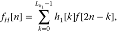
The implementation of 1D wavelet transform by means of multirate filter banks has been developed since the late 1980s. The forward dyadic wavelet transform is formed by a pair of analysis filters ![]() followed by down‐sampling the filtered signals with decimation factor of 2. To reconstruct the signal from the wavelet coefficients (that is, the subband signals), the inverse wavelet transform is performed with zero insertion at every other signal of the subband signals and then filtering the zero‐inserted subband signals with a pair of synthesis filters
followed by down‐sampling the filtered signals with decimation factor of 2. To reconstruct the signal from the wavelet coefficients (that is, the subband signals), the inverse wavelet transform is performed with zero insertion at every other signal of the subband signals and then filtering the zero‐inserted subband signals with a pair of synthesis filters ![]() .
1
These set of filters are also known as the subband filters, and the filter system together with the down‐ and up‐samplers will form a multirate filter system. Subband filters with different cutoff frequencies can be employed to analyze the input signal. In the case of wavelet signal interpolation, a half‐band low‐pass filter
.
1
These set of filters are also known as the subband filters, and the filter system together with the down‐ and up‐samplers will form a multirate filter system. Subband filters with different cutoff frequencies can be employed to analyze the input signal. In the case of wavelet signal interpolation, a half‐band low‐pass filter ![]() (with passband
(with passband ![]() radians) is usually applied to remove all the frequency components that are above half of the highest frequency in the signal. The low‐pass filter
radians) is usually applied to remove all the frequency components that are above half of the highest frequency in the signal. The low‐pass filter ![]() is reducing the signal resolution by half but leaving the scale unchanged. According to Nyquist theorem (Theorem 1.1), the subband signal that has the highest frequency of
is reducing the signal resolution by half but leaving the scale unchanged. According to Nyquist theorem (Theorem 1.1), the subband signal that has the highest frequency of ![]() radians instead of
radians instead of ![]() will only require half of the original samples to represent the signal without loss. As a result, the filtered output is down‐sampled by a factor of 2, simply by discarding every other sample, and the scale of the subband signal is now doubled. The resolution and scale of the approximation subband signal can be further doubled by putting it through the multirate filter bank again. The approximation signal is now filtered with the low‐pass subband filter
will only require half of the original samples to represent the signal without loss. As a result, the filtered output is down‐sampled by a factor of 2, simply by discarding every other sample, and the scale of the subband signal is now doubled. The resolution and scale of the approximation subband signal can be further doubled by putting it through the multirate filter bank again. The approximation signal is now filtered with the low‐pass subband filter ![]() , whose passband is just half of the previous filter bandwidth, and the subsequent down‐sampling by a factor of 2 will change the scale once again. As a result, the signal is being decomposed into subband signals with descending resolutions (as the detail subbands keep down‐sampling). Such decrease in resolution and increase in scale will be repeated as shown in Figure 6.1 until a coarse description of the signal is achieved at a desired level. Note that the spectral responses of the analysis subband filters have finite transition regions and will overlap with one another, as shown in Figure 6.2 , which means that the down‐sampling and up‐sampling processes will introduce aliasing distortion into the subband signals and the reconstructed signal. To eliminate the aliasing distortion in the reconstructed signal, the synthesis and analysis filters need to have certain relationships such that the aliased components in the transition regions will be canceled by the synthesis filters. While the perfect reconstruction condition will be discussed in Section 6.1.1 , the subband filters must also satisfy other conditions before a multi‐resolution analysis (wavelet analysis) can be achieved, which will be discussed in Section 6.1.2 .
, whose passband is just half of the previous filter bandwidth, and the subsequent down‐sampling by a factor of 2 will change the scale once again. As a result, the signal is being decomposed into subband signals with descending resolutions (as the detail subbands keep down‐sampling). Such decrease in resolution and increase in scale will be repeated as shown in Figure 6.1 until a coarse description of the signal is achieved at a desired level. Note that the spectral responses of the analysis subband filters have finite transition regions and will overlap with one another, as shown in Figure 6.2 , which means that the down‐sampling and up‐sampling processes will introduce aliasing distortion into the subband signals and the reconstructed signal. To eliminate the aliasing distortion in the reconstructed signal, the synthesis and analysis filters need to have certain relationships such that the aliased components in the transition regions will be canceled by the synthesis filters. While the perfect reconstruction condition will be discussed in Section 6.1.1 , the subband filters must also satisfy other conditions before a multi‐resolution analysis (wavelet analysis) can be achieved, which will be discussed in Section 6.1.2 .
![Schematic of 1D DWT decomposition with arrows from f[n] pointing to h1(n) and h0(n), from h1(n) to fH1[n], from h0(n) to fL1[n] branching to h1(n) and h0(n), from h1(n) to fH2[n], and from h0(n) to fL2[n].](http://images-20200215.ebookreading.net/2/1/1/9781119119616/9781119119616__digital-image-interpolation__9781119119616__images__c06f001.jpg)
Figure 6.1 Illustration of 1D DWT decomposition. The bandwidth of the resulting signal is marked with “BW.”
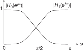
Figure 6.2 Spectral response of a typical perfect reconstruction two‐channel subband filter bank.
6.1.1 Perfect Reconstruction
To understand how to achieve an aliasing free reconstruction of the signal from the subband signals obtained by nonideal analysis subband filters, let us consider a two‐band filter bank, as shown in Figure 6.1 . To simplify our discussions, let us consider the 1D signal ![]() being processed by subband filters shown in Figure 6.1 . The signal
being processed by subband filters shown in Figure 6.1 . The signal ![]() is filtered in parallel by a low‐pass filter
is filtered in parallel by a low‐pass filter ![]() and a high‐pass filter
and a high‐pass filter ![]() at each level of the wavelet decomposition. The two output subband signals are then down‐sampled by dropping the alternate output samples in each signal sequence to produce the low‐pass subband
at each level of the wavelet decomposition. The two output subband signals are then down‐sampled by dropping the alternate output samples in each signal sequence to produce the low‐pass subband ![]() (approximate signal) and high‐pass subband
(approximate signal) and high‐pass subband ![]() (detail signal) as shown in Figure 6.1 . The above arithmetic computation can be expressed as
(detail signal) as shown in Figure 6.1 . The above arithmetic computation can be expressed as

where ![]() and
and ![]() are the lengths of the low‐pass (
are the lengths of the low‐pass (![]() ) and high‐pass (
) and high‐pass (![]() ) filters, respectively. The low‐pass subband
) filters, respectively. The low‐pass subband ![]() is low‐resolution approximation of the input signal
is low‐resolution approximation of the input signal ![]() . As a result, applying the above analysis to decompose the signal
. As a result, applying the above analysis to decompose the signal ![]() , which will generate
, which will generate ![]() and
and ![]() . Note that we have expanded the subband signals to include the superscript 2 to indicate the level of decomposition. As a result,
. Note that we have expanded the subband signals to include the superscript 2 to indicate the level of decomposition. As a result, ![]() and
and ![]() will be the same as
will be the same as ![]() and
and ![]() . This multi‐resolution decomposition approach is shown in Figure 6.1 for two‐level decomposition. This decomposition can be iteratively applied to all the low‐pass subband signal until the
. This multi‐resolution decomposition approach is shown in Figure 6.1 for two‐level decomposition. This decomposition can be iteratively applied to all the low‐pass subband signal until the ![]() level low‐pass subband signal
level low‐pass subband signal ![]() is obtained. During the inverse transform, both
is obtained. During the inverse transform, both ![]() and
and ![]() in the lowest level (the highest
in the lowest level (the highest ![]() of the subband signals in concern) are up‐sampled by inserting zeros between every two samples and then filtering the zero‐inserted subband signal sequences by the synthesis low‐pass filter
of the subband signals in concern) are up‐sampled by inserting zeros between every two samples and then filtering the zero‐inserted subband signal sequences by the synthesis low‐pass filter ![]() and high‐pass filter
and high‐pass filter ![]() . The two output signal sequences are added together to obtain the subband signal
. The two output signal sequences are added together to obtain the subband signal ![]() at a higher level as shown in Figure 6.1 . This process will continue until level 0 to obtain the reconstructed signal
at a higher level as shown in Figure 6.1 . This process will continue until level 0 to obtain the reconstructed signal ![]() , which has the same resolution/scale as that of
, which has the same resolution/scale as that of ![]() . It should be noted that the hat in the symbol
. It should be noted that the hat in the symbol ![]() indicates it is a reconstructed signal for the ease of discussion without ambiguity. The multirate filter bank is said to be a perfect reconstruction system if and only if
indicates it is a reconstructed signal for the ease of discussion without ambiguity. The multirate filter bank is said to be a perfect reconstruction system if and only if ![]() is a shifted version of
is a shifted version of ![]() , which in turn requires the subband filters to satisfy the power complementary condition.
, which in turn requires the subband filters to satisfy the power complementary condition.
There are infinitely many subband filters that form perfect reconstruction filter banks. The built‐in perfect reconstruction filter bank families in MATLAB include Daubechies (db), Coiflets (coif), Symlets (sym), Discrete Meyer (dmey), and Reverse Biorthogonal (rbio). In MATLAB's convention, the number that follows the mother wavelet family name is the subband filter length. As an example, db1 is the length 1 Daubechies subband filter, which is also known as the Haar wavelet. In this chapter, we choose the Haar wavelet, because it is the simplest and yet works just as good as other wavelets.
6.1.2 Multi‐resolution Analysis
Not all perfect reconstruction subband filter banks can form wavelet transform. The analysis low‐pass subband filter has to satisfy the orthonormality constraint, such that ![]() . Furthermore, it must have at least one vanishing moment, which implies
. Furthermore, it must have at least one vanishing moment, which implies ![]() . The infinite product of such subband filter,
. The infinite product of such subband filter, ![]() , will converge to a function
, will converge to a function ![]() whose inverse Fourier transform is the continuous time function
whose inverse Fourier transform is the continuous time function ![]() known as the scaling function. The scaling function
known as the scaling function. The scaling function ![]() is the solution to the dilation equation.
is the solution to the dilation equation.
and it is orthogonal to its integer translates. The scaling function determines the wavelet function ![]() by means of the analysis high‐pass subband filter
by means of the analysis high‐pass subband filter ![]() with
with
The set of functions obtained from the dilation and translation of ![]() as
as ![]() forms a tight frame in
forms a tight frame in ![]() . In other words, the span of dilates and translates of the scaling function
. In other words, the span of dilates and translates of the scaling function ![]() forms a series of subspace
forms a series of subspace ![]() in
in ![]() .
.
Since ![]() spans
spans ![]() , therefore, any continuous time function
, therefore, any continuous time function ![]() can be expanded as a linear combination of the scaling function as
can be expanded as a linear combination of the scaling function as
where the superscript “0” denotes the expansion coefficient ![]() obtained with the scaling function at scale 0. In dyadic decomposition, the function
obtained with the scaling function at scale 0. In dyadic decomposition, the function ![]() will be subsequently decomposed into coarse‐scale components with the functions in subspace
will be subsequently decomposed into coarse‐scale components with the functions in subspace ![]() and details at several intermediate scales (from 1 to
and details at several intermediate scales (from 1 to ![]() ). A coarse approximation of the function
). A coarse approximation of the function ![]() at scale
at scale ![]() is given by
is given by
which is implemented as low‐pass filtering followed by down‐sampling in the two‐channel subband filter bank. The details are provided by the wavelet function and are computed with the high‐pass filter ![]() . These subspaces have the relation of
. These subspaces have the relation of
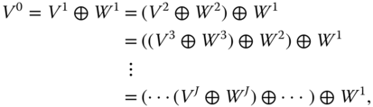
as shown in Figure 6.3 .
![Schematic of multi-resolution space representation with 3 concentric ovals labeled V2, W2, and W1 (inner-outer) with outer and middle ovals pointed by arrows labeled V0 = V1 + W1 = [V2 + W2] + W1 and V1 = V2 + W2, respectively.](http://images-20200215.ebookreading.net/2/1/1/9781119119616/9781119119616__digital-image-interpolation__9781119119616__images__c06f003.jpg)
Figure 6.3 Multi‐resolution space representation.
Besides the orthonormality constraint and the vanishing moment constraint, the wavelet transform usually forms an orthogonal transform, such that the analysis subband filters and synthesis subband filters are the same set of filters. Except the very special Haar wavelet, there do not exist any other subband filters that can form a perfect reconstruction orthogonal filter bank, while the subband filters also have linear phase. On the other hand, the human visual system has shown to be very sensitive to signal phase distortion. Therefore, it is very important to use linear phase subband filters. A way to achieve perfect reconstruction with linear phase subband filters is to allow the analysis subband filters and the synthesis subband filters to be different. Such multirate filter bank system will form a biorthogonal wavelet transform. The extra freedom in the design of biorthogonal subband filters will allow more accurate design of the low‐pass filter to suit for particular image processing problem. On the other hand, departure from orthogonality generally has a negative impact on the signal representation efficiency. It has found that biorthogonal bases that closely resemble orthonormal bases are suitable for image processing application. The wavelet filters chosen for image compression in JPEG2000 are the biorthogonal 9/7 and 5/3 subband filters that are nearly orthogonal [4 ]. A filter bank with the two subband filters' length of 7 and 9 can have 6 and 2 vanishing moments or 4 and 4 vanishing moments as in the case of JPEG2000 wavelet. The same wavelet is also known as the Daubechies 9/7 (based on filter size) or biorthogonal 4.4 (based on vanishing moments). Nevertheless, this chapter will concentrate on the application of Haar wavelet for image interpolation, as it is the easiest to work with and can still provide very good interpolation results. Furthermore, it helps to explain the concepts clearly without messing with the forward and backward DWT transformation programming difficulties.
6.1.3 2D Wavelet Transform
The 2D DWT on the image ![]() can be computed by first performing 1D DWT (horizontally) on the rows. Then we perform the same 1D DWT on the columns (vertically) for both the low‐pass and high‐pass subband signals obtained in the horizontal analysis as shown in Figure 6.4 with the Cat image as an example. As a result, there will be four subband images
can be computed by first performing 1D DWT (horizontally) on the rows. Then we perform the same 1D DWT on the columns (vertically) for both the low‐pass and high‐pass subband signals obtained in the horizontal analysis as shown in Figure 6.4 with the Cat image as an example. As a result, there will be four subband images ![]() ,
, ![]() ,
, ![]() , and
, and ![]() , where the
, where the ![]() and
and ![]() follow the same notations as that in 1D DWT with the superscript indicating wavelet decomposition, where the superscript “1” refers to 1‐level wavelet decomposition. Needless to say, we assume that the subband filter kernels of the 2D DWT are separable so that the wavelet decomposition can be carried out along the rows and columns separately. The decomposed subband images have a total size equal to that of the original image, which can be observed from Figure 6.4 c with all the subband images that are stitched together to form one image. The multi‐resolution analysis will repeat the operation on the
follow the same notations as that in 1D DWT with the superscript indicating wavelet decomposition, where the superscript “1” refers to 1‐level wavelet decomposition. Needless to say, we assume that the subband filter kernels of the 2D DWT are separable so that the wavelet decomposition can be carried out along the rows and columns separately. The decomposed subband images have a total size equal to that of the original image, which can be observed from Figure 6.4 c with all the subband images that are stitched together to form one image. The multi‐resolution analysis will repeat the operation on the ![]() subband image as the input image for further decomposition. A 2‐level wavelet decomposition of the Cat image is illustrated in Figure 6.4 d using the MATLAB wavelet toolbox function
subband image as the input image for further decomposition. A 2‐level wavelet decomposition of the Cat image is illustrated in Figure 6.4 d using the MATLAB wavelet toolbox function dwt2 as in Listing 6.1.1, and the stitched image from all the subband images obtained from the two levels of decompositions is shown in Figure 6.4 e. Note that in order to display all the subband images with the same dynamic range, the pixels of all the subband images, except ![]() , have been scaled by performing
, have been scaled by performing log10 and multiplying the result with 50 for those in the first‐level decomposition and 100 for those in the second level of decomposition, as shown in Listing 6.1.1. It should be noted that the superscript “2” of ![]() indicates it is a 2‐level wavelet decomposed low‐pass subband image. Similarly, the superscript convention can be applied to the symbols of the other 2‐level subband images.
indicates it is a 2‐level wavelet decomposed low‐pass subband image. Similarly, the superscript convention can be applied to the symbols of the other 2‐level subband images.


Figure 6.4 Illustration of 2D wavelet decomposition of the Cat image. (a) Filter bank structure for 2D wavelet image transformation, (b) the corresponding second‐level wavelet decomposition, and (c) the subband stitched together to show the invariance of the overall spatial size, (d) second‐level dyadic decomposition, with (e) the subband images from first‐ and second‐level decomposition stitched together (the subband images look darker because brightness scaling has been applied to squeeze the dynamic range of all subband images to be displayed in the same figure).
The dwt2 performs one‐level wavelet decomposition of the image f using the wavelet defined by the second input parameter, which in this case is db1, the Haar wavelet. The function dwt2 is then applied to LL1 (where LL1 is the subband image ![]() ) again to obtain the second‐level decomposition. Note that the pixels in subband image
) again to obtain the second‐level decomposition. Note that the pixels in subband image LL2 (where LL2 is the subband image ![]() ) have the same dynamic range as that of the original image
) have the same dynamic range as that of the original image f, while all other subband images have small and sparse pixel values. It is vivid from Figure 6.4 e that the 2‐level decomposed subband images ![]() (
(LH2 in MATLAB), ![]() (
(HL in MATLAB), and ![]() (
(HH in MATLAB), contains the horizontal, vertical, and diagonal details of the original image ![]() , respectively. The last line of the codes in Listing 6.1.1 makes use of the
, respectively. The last line of the codes in Listing 6.1.1 makes use of the mat2gray function to normalize the pixel intensity of gLL1 for display purpose. To reconstruct the image from the subband images, we shall make use of idwt2 as in Listing 6.1.2. To simplify the discussion without losing generality, in the rest of the discussions, the superscript on the 1‐level decomposed subband images will be omitted, but that of the 2‐level decomposed subband images would be remained. The same idea would be applied to the MATLAB symbols, e.g. LL and LL1 are both referring to the 1‐level decomposed subband image.
The output of the IDWT function idwt2 is of class double and contains negative and other pixel values outside the dynamic range of the original image f. As a result, some mappings will have to be performed before you can display them as that in Figure 6.4 , where the MATLAB function brightnorm will be used (see Listing 5.3.5).
6.2 Wavelet Image Interpolation
Consider the DWT of a 1D high‐resolution signal ![]() with a bandwidth support of
with a bandwidth support of ![]() as shown in Figure 6.5 . This high‐resolution signal
as shown in Figure 6.5 . This high‐resolution signal ![]() is decomposed into the low frequency component
is decomposed into the low frequency component ![]() and high frequency component
and high frequency component ![]() as shown in the figure. However, only the low frequency subband signal
as shown in the figure. However, only the low frequency subband signal ![]() is available, while the high frequency subband signal
is available, while the high frequency subband signal ![]() is missing. A high‐resolution signal
is missing. A high‐resolution signal ![]() that approximates
that approximates ![]() can be obtained by computing the inverse discrete wavelet transform (IDWT) of
can be obtained by computing the inverse discrete wavelet transform (IDWT) of ![]() together with an estimation of the high frequency subband component
together with an estimation of the high frequency subband component ![]() using
using ![]() as shown in Figure 6.5 . In a similar manner, the 2D DWT of a high‐resolution image
as shown in Figure 6.5 . In a similar manner, the 2D DWT of a high‐resolution image ![]() with missing high frequency subband images (
with missing high frequency subband images (![]() ,
, ![]() , and
, and ![]() ) can be approximated by computing the 2D IDWT using the low‐resolution subband image
) can be approximated by computing the 2D IDWT using the low‐resolution subband image ![]() and the estimation of the missing subband images. Readers should be able to understand that this is the same as recasting the interpolation problem to a subband image estimation problem, where the given low‐resolution image
and the estimation of the missing subband images. Readers should be able to understand that this is the same as recasting the interpolation problem to a subband image estimation problem, where the given low‐resolution image ![]() enumerates
enumerates ![]() , with the unknown
, with the unknown ![]() ,
, ![]() , and
, and ![]() being estimated. As a result, the IDWT of
being estimated. As a result, the IDWT of ![]() together with the estimated
together with the estimated ![]() ,
, ![]() , and
, and ![]() will construct
will construct ![]() , an approximation to the high‐resolution image
, an approximation to the high‐resolution image ![]() , which in turn is the interpolated image of the low‐resolution image
, which in turn is the interpolated image of the low‐resolution image ![]() . In the following discussion, we shall denote the
. In the following discussion, we shall denote the ![]() ,
, ![]() ,
, ![]() , and
, and ![]() as
as ![]() ,
, ![]() ,
, ![]() , and
, and ![]() subband images for simplicity in this section. It should be noted that the two sets of symbols would be interchangeably used.
subband images for simplicity in this section. It should be noted that the two sets of symbols would be interchangeably used.

Figure 6.5 Image interpolation by wavelet coefficient estimation.
6.2.1 Zero Padding
The simplest DWT interpolation method is discrete wavelet transform zero padding (DWT‐ZP), where the low‐resolution image will enumerate the ![]() subband image, while the other three subband images (
subband image, while the other three subband images (![]() ,
, ![]() , and
, and ![]() ) are padded with zeros. This kind of high frequency subband image estimation method hits off with the observation that the pixel values of the high frequency subband images are usually very small, which hints that replacing the high frequency subband images with zero matrices will not cause much information loss. The IDWT of the zero‐padded subband images will have to be multiplied with a scaling factor to restore the brightness of the reconstructed image to be compatible with that of the given low‐resolution image. Depending upon the implementation of the DWT, the system will have a different DC gain for the low‐pass filter and Nyquist gain for the high‐pass filter, which will result in different scaling factors. In our example, we choose to use
) are padded with zeros. This kind of high frequency subband image estimation method hits off with the observation that the pixel values of the high frequency subband images are usually very small, which hints that replacing the high frequency subband images with zero matrices will not cause much information loss. The IDWT of the zero‐padded subband images will have to be multiplied with a scaling factor to restore the brightness of the reconstructed image to be compatible with that of the given low‐resolution image. Depending upon the implementation of the DWT, the system will have a different DC gain for the low‐pass filter and Nyquist gain for the high‐pass filter, which will result in different scaling factors. In our example, we choose to use db1, the Haar wavelet, where the subband filters with both DC and Nyquist gain equal to ![]() (the orthonormality constraint as discussed in Section 6.1.2 ). This will help to maintain all four subband images to have the same dynamic range. Consequently, the scaling factor will be 2, which is the multiplication of the squares of the DC gain. The MATLAB source Listing 6.2.1 implements the DWT zero padding image interpolation with
(the orthonormality constraint as discussed in Section 6.1.2 ). This will help to maintain all four subband images to have the same dynamic range. Consequently, the scaling factor will be 2, which is the multiplication of the squares of the DC gain. The MATLAB source Listing 6.2.1 implements the DWT zero padding image interpolation with db1 wavelet. Note that the scaling factor of 2 is applied to the idwt function to obtain the interpolated image ng. Further note that all pixels with negative intensity values will be substituted with zero intensity and the final image array is cast to unit8 to obtain the final interpolated image ![]() .
.

The interpolation result of the Cat image shown in Figure 6.6 can be obtained by the following MATLAB function call:
![]()

Figure 6.6 Cat image interpolated with Haar wavelet zero padding and the zoom‐in sub‐images of the Cat whiskers in (c) and ear in (e), while shown in (b) and (d) are the sub‐images of the same area extracted from the original high‐resolution Cat image.
Readers may have already noticed that with all the high frequency subband images (![]() ,
, ![]() , and
, and ![]() ) being constrained with zero values, the DWT‐ZP interpolation is essentially the same as the linear interpolation method described in Figure 4.1 with the interpolation kernel given by the subband synthesis filter
) being constrained with zero values, the DWT‐ZP interpolation is essentially the same as the linear interpolation method described in Figure 4.1 with the interpolation kernel given by the subband synthesis filter ![]() . Similar image interpolation performance as that discussed in Chapter 4 is therefore expected, and no advantages of the wavelet multi‐resolution analysis have been made use of.
. Similar image interpolation performance as that discussed in Chapter 4 is therefore expected, and no advantages of the wavelet multi‐resolution analysis have been made use of.
6.2.2 Multi‐resolution Subband Image Estimation
A natural way to exploit the DWT multi‐resolution analysis property is to make use of the multi‐resolution dependency between different levels of wavelet decomposition to estimate the high frequency subband images required for the inverse transform to create the interpolated image. In other words, the high frequency subband images of ![]() (i.e.
(i.e. ![]() ,
, ![]() , and
, and ![]() ) can be estimated from the subband images obtained in higher‐level decomposition. As an example, the bilinear interpolation of the high frequency subband images obtained from the second‐level DWT decomposition of
) can be estimated from the subband images obtained in higher‐level decomposition. As an example, the bilinear interpolation of the high frequency subband images obtained from the second‐level DWT decomposition of ![]() (i.e.
(i.e. dwt(LL,‘db1’)) is applied to estimate the high frequency subband images of the interpolated image ![]() , i.e.
, i.e. ![]() ,
, ![]() , and
, and ![]() in the MATLAB source Listing 6.2.2, where the bilinear interpolation is implemented with the function
in the MATLAB source Listing 6.2.2, where the bilinear interpolation is implemented with the function biinterp listed in MATLAB Listing 4.1.5 discussed in Chapter 4.

The brightnorm function in Listing 6.2.2 has been discussed in Chapter 5 and is applied to normalize the pixel intensity dynamic range of the interpolated image g to be the same as that in image f. The reason why a fixed scaling factor 2 cannot be applied to do the job in wavelet based image interpolation is because we have injected subband images with unknown energy into the estimated high frequency subband images (![]() ,
, ![]() , and
, and ![]() ), and, therefore, the scaling factor is most probably not equal to 2. As one of the interpolation constraints is the interpolated image pixels that correspond to the low‐resolution image should be the same, therefore, we shall normalize the interpolated image to have the same dynamic range as that of the low‐resolution image and hence the brightness normalization function.
), and, therefore, the scaling factor is most probably not equal to 2. As one of the interpolation constraints is the interpolated image pixels that correspond to the low‐resolution image should be the same, therefore, we shall normalize the interpolated image to have the same dynamic range as that of the low‐resolution image and hence the brightness normalization function.
The interpolated Cat image using MATLAB source Listing 6.2.2 with the following MATLAB function call is shown in Figure 6.7 :
![]()

Figure 6.7 (a) Cat image interpolated with Haar wavelet with high frequency subband images obtained from bilinear interpolation of lower‐level high frequency subband images and the zoom‐in sub‐images of the Cat whiskers in (c) and ear in (e), while shown in (b) and (d) are the sub‐images of the same area extracted from the interpolated image obtained by Haar wavelet zero padding.
There are some improvement on the high frequency regions of the interpolated image when compared with that of Figure 6.6 , such that the edges of the interpolated image are not as blur as that in Figure 6.6 . On the other hand, it is not difficult to notice that there is high frequency noise, similar to impulsive noise, in the texture‐rich region of the interpolated image. Heavy ringing artifacts and salt and pepper noises can also be observed in the texture‐rich region of Figure 6.7 . To understand why interpolating the high frequency subband images does not work well in the overall interpolated image, we shall consider the pixel relationship between a given high‐resolution image ![]() and its four subband images obtained by Haar wavelet first‐level DWT analysis.
and its four subband images obtained by Haar wavelet first‐level DWT analysis.


It is vivid that the low‐resolution subband image is the average of the pixels in the high‐resolution image, while the coefficients of high‐resolution subband images are the pixel difference of the high‐resolution image. If we correlate the similarity between the low‐resolution images ![]() and these subband images, their relationship can be represented by Taylor series. A good approximation of the high frequency subband images will assist us to reconstruct a high‐resolution image that approximates the actual high‐resolution image well.
and these subband images, their relationship can be represented by Taylor series. A good approximation of the high frequency subband images will assist us to reconstruct a high‐resolution image that approximates the actual high‐resolution image well.
As discussed in Section 6.2.1 , the ![]() subband image of the high‐resolution image
subband image of the high‐resolution image ![]() should be equal to
should be equal to ![]() (i.e.
(i.e. ![]() in Eq. (6.10 )). To approximate the high frequency subband images, we shall consider the first‐order Taylor series expansion of the high‐resolution image
in Eq. (6.10 )). To approximate the high frequency subband images, we shall consider the first‐order Taylor series expansion of the high‐resolution image ![]() , which yields
, which yields
where ![]() and
and ![]() are the first‐order derivatives along
are the first‐order derivatives along ![]() and
and ![]() , respectively, and
, respectively, and ![]() . Consider the
. Consider the ![]() subband image
subband image
where similar analysis is also considered in [17 ]. Rewriting ![]() and
and ![]() and applying the Taylor series expansion on
and applying the Taylor series expansion on ![]() in Eq. (6.14 ) yields
in Eq. (6.14 ) yields
which implies
As a result, we shall approximate
In similar manner, the ![]() subband image is given by
subband image is given by
Again, considering ![]() and
and ![]() , the
, the ![]() subband image can be rewritten as
subband image can be rewritten as
The Taylor series expansion of ![]() in Eq. ( 6.14
) yields
in Eq. ( 6.14
) yields

Further note that
where ![]() . The above equation implies
. The above equation implies
or equivalently
This relationship is invariant with shifting by 2 along both ![]() and
and ![]() . Therefore,
. Therefore,
Substituting Eqs. (6.25 ) and (6.26 ) into (6.20 ) yields

which is the difference between the means of two column pixels separated by one column apart, and each column has two components. Consider that the decimation of the means of the pixels will yield ![]() . As a result, Eq. (6.27 ) is equivalent to the computation of the horizontal difference (along
. As a result, Eq. (6.27 ) is equivalent to the computation of the horizontal difference (along ![]() direction) between adjacent
direction) between adjacent ![]() , which is equivalent to
, which is equivalent to ![]() of the first‐level Haar wavelet decomposition of
of the first‐level Haar wavelet decomposition of ![]() . In other words, the
. In other words, the ![]() from the 2‐level wavelet decomposition of
from the 2‐level wavelet decomposition of ![]() is a good approximation of
is a good approximation of ![]() . With
. With ![]() with even
with even ![]() and
and ![]() , the missing
, the missing ![]() with either
with either ![]() or
or ![]() or both being odd has to be estimated. There exists a lot of estimation method for these missing
or both being odd has to be estimated. There exists a lot of estimation method for these missing ![]() subband image pixels, and we have tried the bilinear interpolation in MATLAB Listing 6.2.2, which does not give good result in general. As a result, the most straight forward method has been proposed in [62 ], which padded the unknown pixels in
subband image pixels, and we have tried the bilinear interpolation in MATLAB Listing 6.2.2, which does not give good result in general. As a result, the most straight forward method has been proposed in [62 ], which padded the unknown pixels in ![]() with zero for either
with zero for either ![]() or
or ![]() or both being odd. Similar relationship is derived for the
or both being odd. Similar relationship is derived for the ![]() subband image. This forms the alternate zero padding wavelet image interpolation method. Shown in Figure 6.8 is a synthetic figure that shows the two subband images
subband image. This forms the alternate zero padding wavelet image interpolation method. Shown in Figure 6.8 is a synthetic figure that shows the two subband images ![]() and
and ![]() obtained from alternate zero padding wavelet image interpolation method, while
obtained from alternate zero padding wavelet image interpolation method, while ![]() . Together with
. Together with ![]() , the IDWT result of these four subband images of
, the IDWT result of these four subband images of ![]() will yield the interpolated image.
will yield the interpolated image.

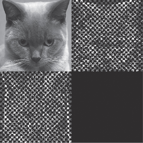
Figure 6.8 Wavelet zero padding image interpolation with alternate zero wavelet coefficient insertion.
The alternate zero padding wavelet interpolation method is implemented in MATLAB Listing 6.2.3 with function name wazp. Similar to the bilinear subband image interpolation‐based wavelet interpolation method (i.e. wbp), the interpolated image normalization factor is affected by the energy of the estimated subband images that we have injected into the IDWT process. In this case, it is image dependent, and, therefore, the brightness normalization function brightnorm is applied to normalize the interpolated image to have the same dynamic range as that of the given low‐resolution image.
The interpolated Cat image obtained from MATLAB source Listing 6.2.3 with the following function call is shown in Figure 6.9 :
![]()

Figure 6.9 (a) Cat image interpolated with alternate zero padding wavelet interpolation and the zoom‐in sub‐images of the Cat whiskers in (c) and ear in (e), while shown in (b) and (d) are the sub‐images of the same area extracted from the original high‐resolution Cat image.
It is vivid that the image edges are not as blur nor noisy as that in Figures 6.6 and 6.7 of wavelet zero padding (WZP) interpolation and wavelet with bilinear interpolated subband images interpolation. The most obvious artifacts in Figure 6.9 are the sudden brightness of the interpolated pixels near the edges of the image, which are perceived as impulsive noise or shot noise.
The unpleasant shot noise is mostly observed to be near the edges of the interpolated image that is caused by excess signal power of the high frequency subband images. A simple test of decreasing the high frequency subband image energy by dividing the subband coefficients by 1.5 as the following MATLAB function wazp15 will confirm the conjecture on the origin of the shot noise.
The interpolated Cat image using MATLAB source Listing 6.2.4 with the following function call is shown in Figure 6.10 :
![]()
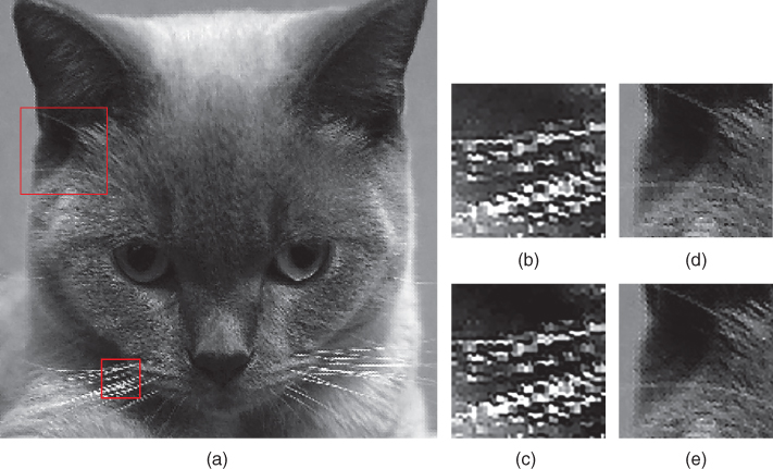
Figure 6.10 (a) Cat image interpolated with alternate zero padding wavelet interpolation and subband images divided by 1.5 and the zoom‐in sub‐images of the Cat whiskers in (c) and ear in (e), while shown in (b) and (d) are the sub‐images of the same area extracted from the interpolated image obtained by alternate zero padding wavelet without scaling the subband images.
It can be observed that most of the shot noise is suppressed when compared with that in Figure 6.9 . At the same time, the edge sharpness is preserved. This result prompted us to investigate the correct scaling of the energy of the estimated high frequency subband images to be applied in the wavelet image interpolation problem. To learn how to scale the estimated high frequency subband images, we have to understand some basic functional analysis using wavelet.
6.2.3 Hölder Regularity
In order to bring a spatial coherence between the spatial image and the wavelet coefficients, the basis of the applied wavelet transform must satisfy a smoothness constraint. A smooth wavelet transform of high‐resolution image will render regions that do not have much high frequency components to have the corresponding wavelet coefficients with very small magnitudes, which can be ignored without affecting the overall quality of the wavelet image representation. However, if a region has edges, the corresponding wavelet coefficients are usually significant, and they cannot be neglected while obtaining the high‐resolution image.
The smoothness of an image can be defined in terms of Hölder regularity of the wavelet transform [22 ]. Functions with a large Hölder exponent will be both mathematically and visually smooth. Locally, an interval with high regularity will be a smooth region, and an interval with low regularity will correspond to roughness, such as at an edge in an image. To extend this concept to image interpolation, the smoothness constraints should be enforced while up‐sampling at relatively smooth regions and enhancing the edges of the interpolated high‐resolution image. Since this chapter is about the application of wavelet to interpolate images, we are trying our best to avoid the functional analysis discussion of wavelet, which we considered to be out of the scope of this book. On the other hand, we do have to bring in the Lipschitz property on functional analysis. The Lipschitz property let us know that the wavelet coefficients for pixels near sharp edges decay exponentially over scale [44 ]. The wavelet analysis of the interpolated image should preserve the regularity during analysis. There are two schools of regularity preservation in wavelet image interpolation.
The first method preserves the energy ratio of the high frequency subband image across scale. In other words, among 1‐level, 2‐level, and 3‐level DWT decomposed ![]() images, their energy, computed as variance of the coefficients in the subband images, should satisfy
images, their energy, computed as variance of the coefficients in the subband images, should satisfy
To put this into implementation, the ![]() subband image should be scaled by the variance ratio of the 1‐level and 2‐level
subband image should be scaled by the variance ratio of the 1‐level and 2‐level ![]() subband images as
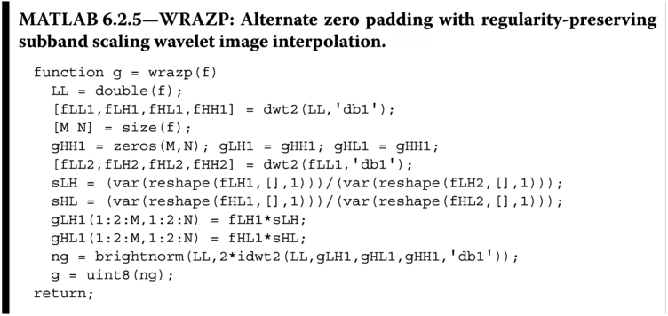
subband images as ![]() . The following MATLAB source modified from Listing 6.2.4 applied the regularity‐preserving property in Eq. (6.28 ) to interpolate image.
. The following MATLAB source modified from Listing 6.2.4 applied the regularity‐preserving property in Eq. (6.28 ) to interpolate image.
The interpolated Cat image obtained by wrazp with the function call
![]()
is shown in Figure 6.11 . It can be observed that almost all shot noise are suppressed in the interpolated image when compared with Figures 6.9 and 6.10 . At the same time, the edge sharpness is preserved.

Figure 6.11 (a) Cat image interpolated with alternate zero padding with regularity‐preserving subband scaling wavelet image interpolation and subband images scaled to satisfy across scale subband image energy ratio and the zoom‐in sub‐images of the Cat whiskers in (c) and ear in (e), while shown in (b) and (d) are the sub‐images of the same area extracted from the original high‐resolution Cat image.
6.2.3.1 Local Regularity‐Preserving Problems
To improve the image interpolation result, the subband image coefficient scaling should be adaptive, such that for those subband coefficients that are identified as strong edges, the energy ratio of the corresponding subband coefficients across scales (where the energy in this case will be the squares of the subband coefficients) will be used to scale the corresponding subband coefficients or even estimate the subband coefficients. This property is first proposed in Mallat's wavelet modulus maxima theory [44 ] that extrapolates wavelet transform extrema across scales and then the regularity‐preserving image interpolation methods in [11 ] and [14 ].
The regularity‐preserving interpolation technique synthesizes a new wavelet subband based on the decay of known wavelet transform coefficients [11 ]. The creation of the high frequency subband image is separated into two separate steps. In the first step, row edges with significant correlation across scales are identified. Then near these edges the rate of decay of the wavelet coefficients is extrapolated to approximate the high frequency subband required to resynthesize a row of twice the original size. In the second step, the same procedure as in the first step is applied to each column of the row interpolated image. There are a number of problems associated with this local regularity‐preserving interpolation method.
Firstly, we shall assume symmetric wavelets are applied to the local regularity‐preserving image interpolation problem. This is because the nonsymmetric wavelets will cause incoherent in the signs and/or locations of the wavelet transform extrema. Let us consider the spatial coherent problem of an edge across three levels of symmetric wavelet decomposition. Consider the case where we try to locate a pixel which has maximum intensity in the third level decomposed subband image. The actual maximum intensity pixel will either locate exactly on the pixel under consideration, or it will locate on the inter‐pixel location between either one of the two neighboring pixels to the pixel under consideration. On the 2 level, there should have corresponding zero crossings. However, due to the down‐sampling operation, the localization of the zero crossing will have four possible pixel locations and also the inter‐pixel locations of these four pixels. Similarly, after up‐sampling, the 1‐level edge location will have a localization of eight possible pixel locations and the nine possible inter‐pixel locations of these eight pixels. As a result, using low‐level wavelet coefficient maxima to determine the edge location at the high‐resolution spatial domain will have very wide ambiguity. Therefore, preserving the regularity through wavelet maxima will cause edge localization problem. In other words, there will be mismatch between the edge locations between the estimated high frequency subband images by lower‐scale subband images and that of the given low‐resolution image. In other words, the generated high‐resolution image will be subjected to artifacts caused by edge mismatch between the low frequency subband image and high frequency subband images, which will be observed as ringing and zigzag noises in the interpolated image.
6.3 Cycle Spinning
Although wavelet interpolation algorithm is not block‐based interpolation algorithm, blocking‐like artifacts (the zigzag artifacts) are observed in the interpolated image. This is caused by the incomparability between the low frequency subband image (the low‐resolution image) and the high frequency subband images. The wavelet transform is shift invariant. However, the forward transform alone and hence the generation of subband images are not. As a result, by making use of the shift variant property, a scheme similar to that in Section 5.4 that averages shifted interpolated images could be developed to suppress zigzag noise. This forms the basis of the cycle spinning wavelet interpolation method presented in [60 ].
There are a number of ways to generate “shifted” high‐resolution images. It can be obtained from removing some rows and columns of an intermediate interpolated image similar to that in Section 5.4. These shifted images are applied with 2D DWT to obtain the subband images of each shifted image. Now we have to decide if we are going to replace the high frequency subband images or the low frequency subband images. The following two sections will discuss the algorithm of each method and their interpolation results.
6.3.1 Zero Padding (WZP‐CS)
The easiest way to generate the shifted high‐resolution images is to perform 2D DWT on the spatially shifted intermediate interpolated image (say, obtained by WRAZP) and then replace the high frequency subband images with zeros. Reconstruct the zero‐padded 2D DWT images (which are equivalent to WZP), and average the result as shown in Figure 6.12 . This is the original cycle spinning method in [60 ], which is the first to consider this approach. A MATLAB implementation of this wavelet zero padding cyclic spinning (WZP‐CS) image interpolation scheme is shown in Listing 6.3.1.

Figure 6.12 WZP‐CS image interpolation signal flow diagram.
Readers might have observed several interesting implementation details in Listing 6.3.1. First, the spatial shifting of the intermediate images is achieved by npart, mpart, and dpart as in Section 5.4. A pseudo block size of four pixels is applied in shifting the high‐resolution image, such that the actual spatial shift is half of the block size and is therefore equal to two pixels. A spatial shift of two pixels in the high‐resolution image is applied because after the decimation process, the low‐resolution subband images of the shifted high‐resolution images will be equivalent to shift the low‐resolution image ![]() by one pixel, which is achieved by
by one pixel, which is achieved by npart, mpart, and dpart with pseudo block size of two pixels.

It can also be noticed that the magnitude of the low frequency subband images is reduced by a factor of 2. This is because the wzp interpolation algorithm will scale the interpolated image with the gain of the subband filter (which is 2). However, the gain of the subband filter is intrinsic to the low‐pass subband image of the 2D DWT images, and, therefore, the extra scaling of 2 has to be taken out from wzp, and hence the division of 2 in the input to the algorithm. The interpolated shifted images are padded with rows and columns of the intermediate subband image to make it the same size as that of the high‐resolution image.
The interpolated image obtained with the function call wzpcs(f) as
is shown in Figure 6.13 . It can be observed that the zigzag noise around the texture‐rich area of the Cat image has been alleviated, especially around the cheek of the Cat. The edges are sharp and with better continuity when compared with all other wavelet image interpolation results discussed so far in this chapter.
![]()
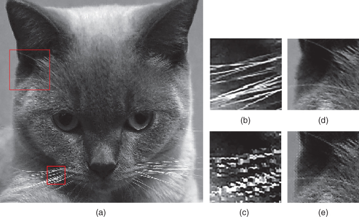
Figure 6.13
(a) Cat image interpolated with wavelet zero padding cyclic spinning image interpolation with intermediate image generated by WRAZP image interpolation through MATLAB function wzpcs and the zoom‐in sub‐images of the Cat whiskers in (c) and ear in (e), while shown in (b) and (d) are the sub‐images of the same area extracted from the original high‐resolution Cat image.
6.3.2 High Frequency Subband Estimation (WLR‐CS)
Another way to generate the spatially shifted high‐resolution images is to perform 2D DWT on the spatially shifted intermediate interpolated image (say, obtained by WRAZP) and then replace the low frequency subband image with the given low‐resolution image ![]() with appropriate spatial shift. The fused DWT subband images will be IDWT to generate the spatially shifted high‐resolution images, which are averaged to obtain the final image. The algorithm is summarized in Figure 6.14 . In this way, the high frequency subband images are preserved, and a better and sharper interpolated image is expected. We shall call this as the wavelet low‐resolution image cyclic spinning (WLR‐CS) image interpolation, because we have fused the spatially shifted (cyclic‐spinned) low‐resolution images to the DWT results of the intermediate image. A MATLAB implementation of the WLR‐CS image interpolation scheme is shown in Listing 6.3.2. It can be observed that the spatial shifting in
with appropriate spatial shift. The fused DWT subband images will be IDWT to generate the spatially shifted high‐resolution images, which are averaged to obtain the final image. The algorithm is summarized in Figure 6.14 . In this way, the high frequency subband images are preserved, and a better and sharper interpolated image is expected. We shall call this as the wavelet low‐resolution image cyclic spinning (WLR‐CS) image interpolation, because we have fused the spatially shifted (cyclic‐spinned) low‐resolution images to the DWT results of the intermediate image. A MATLAB implementation of the WLR‐CS image interpolation scheme is shown in Listing 6.3.2. It can be observed that the spatial shifting in wlrcs is basically the same as that in wzpcs, where the high‐resolution image is shifted horizontally, vertically, and diagonally by two pixels, while the low‐resolution image is shifted similarly by one pixel because of the decimation by a factor of 2 when generating the subband image. It can also be noticed that the magnitude of the low frequency subband images is replaced with the spatially shifted low‐resolution image after scaled by a factor of 2, which is equal to the analysis subband filter gain as discussed in Section 5.1.
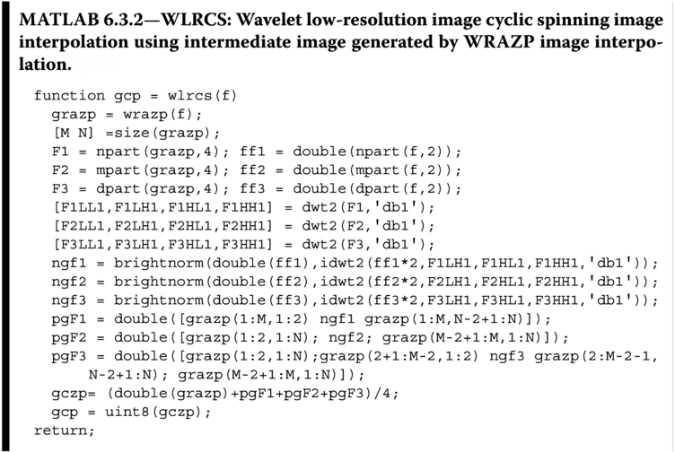

Figure 6.14 Wavelet low‐resolution image cyclic spinning image interpolation signal flow diagram.
The interpolated image obtained from the function call of wlrcs(f) as
![]()
is shown in Figure 6.15 . It can be observed that the zigzag noise around the texture‐rich area of the Cat image has been alleviated, but is not as good as that in Figure 6.13 obtained by wzpcs, especially around the cheek of the Cat. However, the edges are sharper and with better continuity when compared with that of wzpcs. This is because the preservation of high frequency subband images in wlrcs will better preserve the edges not to be blurred by the averaging action in the algorithm. However, preserving the high frequency subband images also means the preservation of the mismatch between the high frequency subband images and the low frequency subband images, and hence the zigzag noise is also preserved in some extent in the interpolated image.

Figure 6.15
(a) Cat image interpolated with wavelet low‐resolution subband cyclic spinning with intermediate image generated by wrazp image interpolation through MATLAB function wlrcs and the zoom‐in sub‐images of the Cat whiskers in (c) and ear in (e), while shown in (b) and (d) are the sub‐images of the same area extracted from the high‐resolution Cat image obtained from wzpcs.
As a compromise, we can also consider averaging the two images obtained from wzpcs and wlrcs as
![]()
It can be observed from the averaged interpolated image in Figure 6.16 that the edges of the image are well defined, without blurring and ringing noise. The texture‐rich area of the image has almost unobservable zigzag noise. The result is almost perfect. Except one thing, this is a fitted high‐resolution image, but not an interpolated high‐resolution image. This is because the low‐resolution image pixel values are not preserved in the high‐resolution image. To correct the fitted high‐resolution image to an interpolated image, we shall turn to iterative error correction technique similar to Section 5.6

Figure 6.16
(a) Interpolated Cat image obtained by averaging wzpcs and wlrcs and the zoom‐in sub‐images of the Cat whiskers in (c) and ear in (e), while shown in (b) and (d) are the sub‐images of the same area extracted from the original high‐resolution Cat image.
6.4 Error Correction
The wavelet‐based image interpolation methods discussed in previous sections (except WZP) interpolate the missing pixels in some way that is consistent with the frequency content of the rest of the signal, which are obtained a priori from the low‐resolution image. As a result, the preservation of the low‐resolution pixel values in the corresponding location of the high‐resolution interpolated image is not guaranteed. In other words, when the high‐resolution interpolated image is directly down‐sampled, the result will be almost sure not to be the same as the given low‐resolution image. This result does not fulfill the low‐resolution pixel value preservation requirement in image interpolation. To make up the differences, we shall perform the error correction method discussed in Section 5.6. The overall error correction method based on WZP is summarized in Figure 6.17 . Readers may have already noticed that we have dropped the word iterative as compared with that in Section 5.6. This is because the WZP that we have applied in the error correction routine is an interpolation method. In other words, the low‐resolution pixel errors will be exactly the same in the corresponding high‐resolution error pixels. In other words, only one iteration will suffice to correct the errors. An implementation of the method that makes use of WZP to interpolate image is shown in MATLAB Listing 6.4.1, where the input to the function wecor is a wavelet fitted high‐resolution image and the original low‐resolution image f. The input image ag can be generated by other wavelet‐based interpolation methods other than WZP. The choice of the generation of the ag using other methods will be left as exercises for the readers.
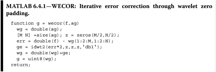
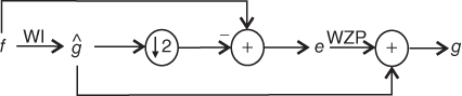
Figure 6.17
Image interpolation by wavelet multi‐resolution synthesis with error correction. (Note: WI can be any wavelet interpolation methods except wzp.)
If we consider the differences between the fitted high‐resolution Cat image ag obtained from ag=wlrcs(f) and the low‐resolution Cat image f, the maximum absolute difference between the down‐sample fitted high‐resolution image ag(1:2:M,1:2:N), where [M N]=size(ag), is 74:
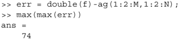
This big difference in the fitted high‐resolution image and the corresponding low‐resolution image can be alleviated by executing
![]()
which will bring the difference down to nil. The resulting image is shown in Figure 6.18 . It can be observed that the blocking artifacts are almost gone, and the edges are sharp. However, new artifacts of small size blocks with alternating brightness are observed in the texture‐rich areas. This is caused by the error image‐induced false edge information. In conclusion, it is nice to obtain an interpolated image using wecor. However, that does come with the scarification of a new type of high frequency noises observable in the texture‐rich area. This makes the engineers to ponder if it is good enough to use the fitted high‐resolution image. The same question will resurface in Chapter 9 when we discuss the fractal image interpolation, which makes use of fractal object to approximate high‐resolution images and is therefore intrinsically a fitting algorithm, not an interpolation algorithm. On the other hand, the fractal object‐based high‐resolution image generation method does show high visual fidelity that cannot be achieved by most methods in literature.

Figure 6.18
(a) Interpolated Cat image obtained by error correcting (wecor) the (wlrcs) wavelet low‐resolution image cyclic spinning high‐resolution image using intermediate image generated by WRAZP image interpolation (wlrcs) and the zoom‐in sub‐images of the Cat whiskers in (c) and ear in (e), while shown in (b) and (d) are the sub‐images of the same area extracted from the original high‐resolution Cat image.
6.5 Which Wavelets to Use
Only the Haar wavelet ‘db1’ is considered in this chapter. Readers may ask if other wavelets give better results to generate a high‐resolution approximation to the given low‐resolution image. To answer this question, we shall have to understand that in wavelet signal analysis, the signal is represented in terms of its coarse approximation at scale ![]() (with basis function
(with basis function ![]() ) and the
) and the ![]() details (with basis function
details (with basis function ![]() ,
, ![]() ). The key to efficient multi‐resolution signal representation by wavelet depends on the properties of the wavelet basis. The three key properties of the wavelet bases are:
). The key to efficient multi‐resolution signal representation by wavelet depends on the properties of the wavelet basis. The three key properties of the wavelet bases are:
-
Regularity: The regularity of scaling function
 has mostly a cosmetic influence on the error introduced by thresholding or quantizing the wavelet coefficients. If
  is smooth, then the generated error is a smooth error. For image interpolation applications, a smooth error is often less visible than an irregular error. Better quality images are obtained with wavelets that are continuously differentiable than those obtained from the discontinuous Haar wavelet. Wavelet regularity increases with the number of vanishing moments. As a result, choosing high regularity wavelet is the same as choosing wavelets with large vanishing moments.
 -
Number of vanishing moments: This affects the amplitude of the wavelet coefficients at fine scale. For smooth regions, wavelet coefficients are small at fine scales if the wavelet has enough vanishing moments to take advantage of the image regularity. A wavelet has
 vanishing moments if and only if its scaling function can generate polynomial of degree smaller than or equal to
  . Both the number of vanishing moments and the regularity of orthogonal wavelets are related, but it is the number of vanishing moments and not the regularity that affects the amplitude of the wavelet coefficients at fine scales [43 ].
 - Kernel size: These need to be reduced to minimize the number of high amplitude coefficients. On the other hand, a large kernel size is required to provide enough vanishing moments. Therefore, the choice of optimal wavelet is a trade‐off between the number of vanishing moments and kernel size.
Every function that satisfies the admissibility condition can be used in a wavelet transform and generates its own wavelets. The ability to approximate signals with a small number of non‐zero coefficients is undoubtedly the key to the success of wavelets for image interpolation. An orthonormal function should also be used such that individual subband signals are independent of each other, and hence the interpolation errors will not propagate across subbands. As a result, orthonormal wavelet with the wavelet transform of an image producing few non‐zero coefficients, which are independent with each subband, is the best wavelet for image interpolation. On the other hand, image interpolation should preserve phase information, as HVS is sensitive to phase error. However, orthogonal wavelets do not have linear phase, except Haar wavelet. Therefore, biorthogonal wavelets with linear phase transform kernel will be the best engineering choice for image interpolation.
In summary, the following listed are the important properties of wavelet functions in image interpolation:
- 1. Compact support (as compact kernel size, which minimizes the high frequency artifacts in the interpolated image and also provides efficient implementation).
- 2. Symmetry (useful in avoiding phase noise in image processing).
- 3. Orthogonality (reduces noise propagation across subbands).
- 4. Regularity and degree of smoothness (improve the smoothness of the interpolation error and hence less visible).
One should choose the wavelet filters based upon the characteristics of the image for suitable perceptual quality. However, the underlying operations in the algorithm are not image content dependent and hence nonadaptive in nature. As a result, should we spend time to choose a specific wavelet with the goal of finding the optimal wavelet for a given image and risking of losing generality? The readers may want to adapt the wavelet image interpolation algorithms discussed in this chapter for image interpolation. But the authors' trial showed that the use of “turnkey” resources provided by MATLAB, in particular the Haar wavelet, will provide just as good image interpolation results as other wavelet transformations.
6.6 Summary
Wavelet transform is an actively pursued area of research. There are many textbooks available for a comprehensive discussion on this topic. The readers are referred to [49 ] for further discussion on wavelet decomposition. The basic wavelet‐based interpolation method is the WZP that interpolates images by zero padding the high frequency subbands (i.e. setting all elements of these subbands to zeros) followed by inverse wavelet transform. WZP has demonstrated to be able to achieve interpolated image with higher PSNR than that achieved by bilinear and bicubic methods. However, visually the method exhibits little difference with conventional convolution‐based method discussed in Chapter 4. The wavelet‐based method seems to sharpen the edges, but the texture‐rich and smooth regions of the image are blurred. This effect is understood because the interpolation step is similar to 1D bilinear interpolation, except at strong edges. To make use of the benefits of wavelet image transformation, the information across wavelet scales should be considered in the interpolation method.
Unlike traditional transform‐based image interpolation methods discussed in Chapter 5, the wavelet‐based interpolation methods give us the flexibility to choose the analysis and synthesis functions. It further allows us to explore the structure of the interpolating image through local Hölder regularity. Wavelet‐based interpolation methods that make use of across scale information and local Hölder regularity information can achieve interpolated images with better PSNR and visually sharpened edges. Having said that, wavelet transform can be performed with any one pair of wavelet transform kernel from an almost infinite number of wavelet transform basis. On the other hand, using wavelets with long kernel will result in interpolated image with image edges being not sharp and smoothed texture‐rich areas. Therefore, most wavelet image interpolation methods make use of simple and short kernel analysis and synthesis basis functions.
Besides the across scale information, the shift variant property of wavelet transformation [15 ] can also be applied to achieve better interpolated image quality. The cycle spinning [60 ] and its variant methods that make use of the wavelet shift variant property have shown to be an effective method against blurring, brokening, and zigzag noise observed on edges.
The last but not the least, readers should understand that except WZP, it is very likely that wavelet‐based image interpolation methods can only achieve a fitted enlarged image instead of an interpolated image. Error correction method has to be applied to constrain the pixels in the fitted high‐resolution image that correspond to the low‐resolution image to have the same pixel intensities. The pro is the increment of the PSNR of the interpolation image. The con is the blocking‐like artifacts because of the brightness mismatch between the low‐resolution image pixel values and the corresponding neighboring pixels in the wavelet interpolated image. Wavelet image fusion technique should be applied to fuse them nicely together to avoid the blocking‐like artifacts, but the fusion technique will usually blur the edges of the interpolated image, and it is therefore required to be handled with care.
6.7 Exercises
- 6.1
Why is the complexity of the 1D discrete wavelet transform linear with
 ?
? - 6.2
Write a function
greducethat takes a square image,img, of size as input, convolves the rows and columns of
 imgwith the filter kernel , and then down‐samples the convolution results to produce an output image of size
  . Demonstrate your function on an image of your choice.
 - 6.3
Write a function
gprojectthat takes a square image,img, of size as input, up‐samples the image to
  , and then convolves the rows and columns of the up‐sampled image with the kernel
  . Demonstrate your function on an image of your choice.
 - 6.4
Write a Laplacian pyramid function
[pyr]=lappry(img,k)that takes a square image,img, as input, and returns a list of images representing the
  levels of a two‐dimensional Laplacian pyramid transformed images. Demonstrate your function's ability by writing a function
 disppyr(pyr,k)that displays the levels of the two‐dimensional Laplacian pyramid using the recursive scheme shown in Figure 6.19 . Demonstrate your function on the Cat image. Note: The image representing the Laplacian pyramid levels must each be normalized to the range [0–255] to construct the display.

Figure 6.19 Laplacian pyramid transform of the Cat. - 6.5
Write a function
g = lappryrecon(pyr,k)to invert a Laplacian pyramid you compute with[pyr]=lappry(im,k)in the above exercise with images stored in the 3D matrix
 pry, and return the reconstructed image. Use the Cat image Laplacian pyramid image sequence in previous exercise, and display the reconstructed image. - 6.6
Multi‐resolution representation can be generated by DCT in a similar way as that of the wavelet transform through reordering the coefficients into subbands as shown in Figure 6.20 . Construct a MATLAB algorithm that takes in an image
im, generate a two‐level multi‐resolution representation of the image using DCT as the basis function, and display it on screen. Note: The HH, HL, and LH subband image levels should be normalized to the range [0–255] with mean gray level equals 128 prior to constructing the display.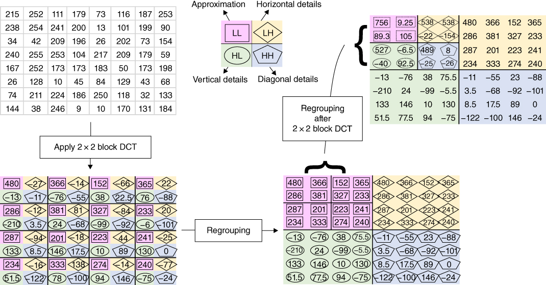
Figure 6.20 Example of reordering of DCT coefficient to form multi‐resolution image representation. (See insert for color representation of this figure.) - 6.7
Compute a three‐level 1D Haar wavelet decomposition of the signal vector
 , and report your finding in the form
  .
. - 6.8
Compare the performance of image interpolation by
wecor(f,ag)for the low‐resolution input imagefand different fitted high‐resolution imageaggenerated by (a)wlrcs, (b)wzpcs, (c)wrazp, and (d)wazp.