4
Nonadaptive Interpolation
There are a number of treatments for the interpolation process in literature. In this book, we adopt the oldest and most widely accepted definition for interpolation that you can find in modern science:
“to insert (an intermediate term) into a series by estimating or calculating it from surrounding known values”
Such a definition of “interpolation” can be found in the Oxford dictionary and can be fulfilled using model‐based signal processing technique. As a result, in digital signal processing, interpolation is also referred to as model‐based recovery of continuous data from discrete samples within a given range of abscissa [61 ]. In the context of digital image, interpolation is further refined to describe the process that estimates the grayscale values of pixels in a particular high density sampling grid with a given set of pixels at a less dense grid, such that the interpolated image is close to the actual analog image sampled with the high density grid. We have discussed the meaning of having two images being “close,” where the closeness can be measured by any objective and subjective metrics as described in Chapter . An example of image interpolation method known as nearest neighbor has been presented in Section 2.7.3, which follows the algorithm shown in Figure 4.1 to generate an image with twice the size (sampling grid with twice the density) as that of the original image. The size expansion is achieved by first increasing the sampling density, such that every ![]() block in the resolution‐expanded image is considered as a local block (with one known pixel at the upper left corner and the rest of pixels with unknown values). The nearest neighbor interpolation method fills up the unknown pixels by replicating the pixels with known values in the local block as shown in Figure 2.26c. This pixel replication method usually results in poor image quality for most natural images, where both peak signal‐to‐noise ratio (PSNR) and Structural SIMilarity (SSIM) are poor, and the interpolated images usually contain visually annoying artifacts, mostly jaggy edges. The pro is its simplicity, which has virtually the lowest computational complexity. Because of this particular advantage, it is still used in a number of imaging equipment. In fact, the trade‐off between interpolation quality and computational complexity is one of the major design considerations in selecting an appropriate image interpolation algorithm for a particular application.
block in the resolution‐expanded image is considered as a local block (with one known pixel at the upper left corner and the rest of pixels with unknown values). The nearest neighbor interpolation method fills up the unknown pixels by replicating the pixels with known values in the local block as shown in Figure 2.26c. This pixel replication method usually results in poor image quality for most natural images, where both peak signal‐to‐noise ratio (PSNR) and Structural SIMilarity (SSIM) are poor, and the interpolated images usually contain visually annoying artifacts, mostly jaggy edges. The pro is its simplicity, which has virtually the lowest computational complexity. Because of this particular advantage, it is still used in a number of imaging equipment. In fact, the trade‐off between interpolation quality and computational complexity is one of the major design considerations in selecting an appropriate image interpolation algorithm for a particular application.
![General framework of image interpolation, with 2 rectangles labeled ↑Γ → Λ and h[m,n] linked by a right arrow labeled ĝ [m,n]. The former is pointed by an arrow labeled f[m,n]. The latter has an arrow labeled g[m,n].](http://images-20200215.ebookreading.net/2/1/1/9781119119616/9781119119616__digital-image-interpolation__9781119119616__images__c04f001.jpg)
Figure 4.1 General framework of image interpolation.
This book is dedicated to the discussion of advanced image interpolation algorithms. Before opening the front curtain of advanced image interpolation algorithms, an overture of classical image interpolation methods based on convolution will be first reviewed in this chapter. While our discussions are general for interpolation ratio ![]() , we shall demonstrate various image interpolation algorithms with an interpolation ratio of 2 whenever we consider appropriate to simplify our discussions.
, we shall demonstrate various image interpolation algorithms with an interpolation ratio of 2 whenever we consider appropriate to simplify our discussions.
4.1 Image Interpolation: Overture
Mere resizing of the image does not increase the image resolution. In fact, resizing should be accompanied by approximations for components with frequencies higher than those representable in the original image and at the same time to obtain higher signal‐to‐noise ratio after the approximations. We may call the process of resizing for the purpose of “increasing the resolution” as up‐sampling or image interpolation. The traditional method of up‐sampling consists of two steps: signal approximation and resampling. Signal approximation is a process to construct a continuous function to represent the original data wherein the original data has to be perfectly coincided with the approximated continuous function. Resampling is a process to map the approximated continuous function with a finer sampling grid by inserting additional sampling points to the approximated curve surface to increase the sample density. In the case of image up‐sampling, all newly added samples are interleaving within the original data and will never be out of the boundary of the original image, while the original data has to be preserved; hence, image up‐sampling is also called image interpolation (not super‐resolution wherein original data may not even exist). In actual implementation, image interpolation of digital image can be considered as a two‐step process: resampling followed by reconstruction, as illustrated in the framework in Figure 4.1 . The former process (resampling) expands the resolution of the original image, ![]() , by mapping it to an expanded image lattice to generate the intermediate image
, by mapping it to an expanded image lattice to generate the intermediate image ![]() . The later process (reconstruction) applies a low‐pass filter to the intermediate image to filter out unwanted high frequency signals or to synthesize the high frequency components, due to lattice expansion to generate a final high‐resolution image
. The later process (reconstruction) applies a low‐pass filter to the intermediate image to filter out unwanted high frequency signals or to synthesize the high frequency components, due to lattice expansion to generate a final high‐resolution image ![]() .
.
The “resampling” process can be mathematically represented by
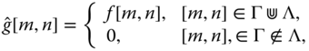
where ![]() and
and ![]() are the low‐resolution and high‐resolution sampling grids, respectively. The MATLAB implementation of the resampling processing is given by the function
are the low‐resolution and high‐resolution sampling grids, respectively. The MATLAB implementation of the resampling processing is given by the function directus listed in Listing 4.1.1.

Increasing the sampling grid density in spatial domain will generate undesired spectral replicas that have to be filtered out with a low‐pass filter ![]() . As discussed in Section 1.1, in the ideal case, the optimal filter
. As discussed in Section 1.1, in the ideal case, the optimal filter ![]() is a discrete sinc function. The practical sinc function cannot have an infinite number of coefficients, but the underlying image
is a discrete sinc function. The practical sinc function cannot have an infinite number of coefficients, but the underlying image ![]() is suffering from aliasing and resulting terrible ringing and undesirable artifacts due to distortion at high frequency components after filtering. Therefore, interpolation using sinc filter is not recommended in image up‐sampling. Different practical choices for the filter
is suffering from aliasing and resulting terrible ringing and undesirable artifacts due to distortion at high frequency components after filtering. Therefore, interpolation using sinc filter is not recommended in image up‐sampling. Different practical choices for the filter ![]() are adopted in practice, such as the zero‐order hold (ZOH), linear and cubic interpolators, etc. These filters try to minimize the spectral leakage at the expense of a wider main lobe. The large main lobe will compromise the resolution of the filtered image and results in blurred image. The design of a good filter
are adopted in practice, such as the zero‐order hold (ZOH), linear and cubic interpolators, etc. These filters try to minimize the spectral leakage at the expense of a wider main lobe. The large main lobe will compromise the resolution of the filtered image and results in blurred image. The design of a good filter ![]() is always a trade‐off between blur and ringing in the up‐sampled image
is always a trade‐off between blur and ringing in the up‐sampled image ![]() . This blur is acceptable if the goal is just to increase the size of the image. Nevertheless, when a better perceived resolution is also required, better approaches that are capable of synthesizing high frequency contents are needed.
. This blur is acceptable if the goal is just to increase the size of the image. Nevertheless, when a better perceived resolution is also required, better approaches that are capable of synthesizing high frequency contents are needed.
The reconstruction process can be considered as a 2D filtering process discussed in Section 2.4, where the resampled image ![]() is convolved with the low‐pass filter
is convolved with the low‐pass filter ![]() . Recalling Eq. (2.17), the reconstruction process in Figure 4.1 is formulated as
. Recalling Eq. (2.17), the reconstruction process in Figure 4.1 is formulated as
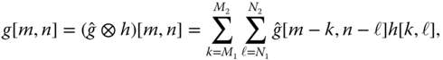
where the range of the convolution is determined by both the data array size and the kernel size of the filter. The pixel values of the newly added samples via resampling will be obtained through convolution. Therefore, the low‐pass filter ![]() is also known as the interpolation kernel. The interpolation kernel is a major factor that affects the quality of the reconstructed image. Many interpolation kernels have been proposed and analyzed in literature, which have different interpolation quality and computational complexity, such that certain trade‐off between the processing time and reconstruction quality will have to be made to select the best interpolation kernel for your application. As an example, more satisfactory interpolation results can be obtained by using interpolation kernel that can smooth the jaggedness of the interpolated image when compared with that obtained by nearest neighbor interpolation method. In this section we describe some of the most well‐known convolution‐based interpolation techniques. Although the convolution kernels of each technique are different, they do share some common characteristics, which shall also be reviewed in Section 4.1.1 . We shall also review the implementation of different interpolation kernels in practice, which applies MATLAB built‐in matrix manipulation functions to ease the entire interpolation process and possibly accomplish the resampling and reconstruction in one single step.
is also known as the interpolation kernel. The interpolation kernel is a major factor that affects the quality of the reconstructed image. Many interpolation kernels have been proposed and analyzed in literature, which have different interpolation quality and computational complexity, such that certain trade‐off between the processing time and reconstruction quality will have to be made to select the best interpolation kernel for your application. As an example, more satisfactory interpolation results can be obtained by using interpolation kernel that can smooth the jaggedness of the interpolated image when compared with that obtained by nearest neighbor interpolation method. In this section we describe some of the most well‐known convolution‐based interpolation techniques. Although the convolution kernels of each technique are different, they do share some common characteristics, which shall also be reviewed in Section 4.1.1 . We shall also review the implementation of different interpolation kernels in practice, which applies MATLAB built‐in matrix manipulation functions to ease the entire interpolation process and possibly accomplish the resampling and reconstruction in one single step.
4.1.1 Interpolation Kernel Characteristics
Before we step into the details of different interpolation kernels, let us take a look of their general characteristics. To accommodate the needs of different image applications, different interpolation kernels can be adopted. However, to minimize the undesirable distortion on the final image, a good convolution kernel, ![]() , should process the following properties to achieve the desired interpolation results:
, should process the following properties to achieve the desired interpolation results:
-
Translation invariance: Given a translation operator
 , where
  with
with  , the interpolation kernel
  should satisfy
(4.3)
should satisfy
(4.3)
-
Rotation invariance: Given a rotation operator
 , where
 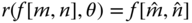 with rotation angle
  ,
(4.4)
,
(4.4)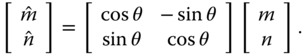
The interpolation kernel
 should satisfy(4.5)
-
Grayscale shift invariance: Given any integer
 , the grayscale intensity shifting is given by
  . The interpolation kernel
  should satisfy
(4.6)
should satisfy
(4.6)
-
Grayscale scale invariance: Given any integer
 , the grayscale intensity scaling is given by
  . The interpolation kernel
  should satisfy
(4.7)
should satisfy
(4.7)
Obviously the above requirements are fulfilled by the linear convolution operator with a symmetric convolution kernel. Further discussions in this book will reveal that the type, size, and shape of the interpolation kernel (either convolution or other types of interpolation methods) will also be major factors that contribute to the quality of the interpolation results. We shall also discuss how these characteristics are adopted in image processing application. In the following sections, we shall introduce a number of traditional and yet still very popular convolution kernels used in image interpolation. They have been shown to be very effective and produce high quality interpolation results for certain types of input images. To simplify the discussion, the interpolation ratio is limited to 2 in the following sections (![]() ).
).
4.1.2 Nearest Neighbor
Nearest neighbor technique uses the grayscale value from the nearest pixel, which is also known as pixel replication technique. The nearest neighbor kernel can be expressed as
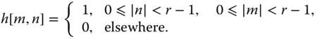
In the case of ![]() , the kernel size is
, the kernel size is ![]() rectangular function. It should be noted that the kernel size is interpolation ratio dependent.
rectangular function. It should be noted that the kernel size is interpolation ratio dependent.
The nearest neighbor interpolation begins with spatial domain resampling to map the original image from the image lattice (![]() ) to an expanded lattice (
) to an expanded lattice (![]() ) as depicted in Eq. (4.1 ) and realized by padding zeros to the original image in every alternative row and column to generate an intermediate image
) as depicted in Eq. (4.1 ) and realized by padding zeros to the original image in every alternative row and column to generate an intermediate image ![]() (an example can be seen in Section 2.7.1). This kind of resampling is regarded to be resolution expansion in spatial domain, which will be adopted for other spatial domain image interpolations to be discussed in this book.
(an example can be seen in Section 2.7.1). This kind of resampling is regarded to be resolution expansion in spatial domain, which will be adopted for other spatial domain image interpolations to be discussed in this book.
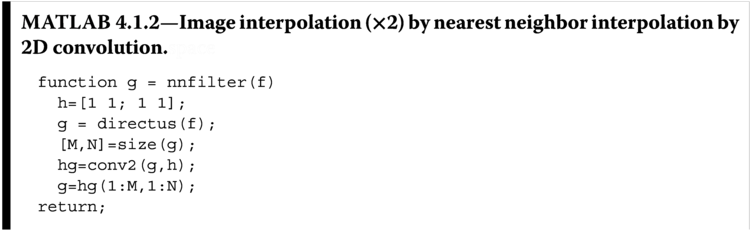
The MATLAB function nnfilter listed in Listing 4.1.2 implements the nearest neighbor interpolation by 2D interpolation. The low‐resolution image f is first zero padded by the function directus. Then the zero‐padded pixels will be assigned with new grayscale values based on the results of the convolution of the intermediate image ![]() and the interpolation kernel
and the interpolation kernel ![]() as depicted in Eq. (4.2 ), thus producing the final image
as depicted in Eq. (4.2 ), thus producing the final image ![]() . It is vivid that the convolution of
. It is vivid that the convolution of ![]() and
and ![]() will suffer from boundary effect, and thus the size of the convolution result will be bigger than that of the desired
will suffer from boundary effect, and thus the size of the convolution result will be bigger than that of the desired ![]() image size. The last row of command in
image size. The last row of command in nnfilter extracts the correctly interpolated image from the convolution result.
The implementation in Listing 4.1.2 is a direct implementation of the nearest neighbor interpolation through theoretical derivation of Eq. ( 4.2
). However, for the sake of simple implementation, and also for computational efficiency, we shall also exploit the implementation of nearest neighbor interpolation in spatial domain with the application of the built‐in array manipulation functions in MATLAB to accomplish the resampling and reconstruction in few lines of codes. Listing 4.1.3 shows the user‐defined MATLAB function (nn) that implements the nearest neighbor interpolation for the up‐sampling ratio ![]() .
.
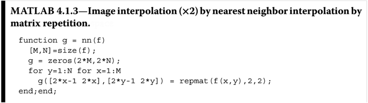
The row and column dimensions of the low‐resolution input image ![]() are first retrieved by the built‐in function
are first retrieved by the built‐in function size and stored in the variables M and N, respectively. The high‐resolution image g is initiated as a zero matrix of the same size as that of the desired interpolated image ![]() through
through g = zeros(2*M,2*N) with ![]() being set to 2. The nested loops in the function is the core for the pixel replication, wherein the built‐in function
being set to 2. The nested loops in the function is the core for the pixel replication, wherein the built‐in function repmat replicates the pixel value in the coordinate [x,y] in the low‐resolution image f to form a ![]() block. The pixel replication can be illustrated mathematically by
block. The pixel replication can be illustrated mathematically by ![]() with
with

The corresponding block in the zero matrix (at location [2*x‐1 2*x],[2*y‐1 2*y]) will be overwritten with the replicated pixel block. It is vivid from Eq. (4.9 ) that the nearest neighbor is a zero‐order polynomial interpolation scheme and is graphically illustrated in Figure 4.2 . Figure 4.3 shows a numerical example to illustrate the implementation of the nearest neighbor interpolation, where a ![]() image is considered to be the original image
image is considered to be the original image ![]() . The image
. The image ![]() has four pixels, and they are assigned with the values of “1”–“4” as shown in Figure 4.3 . The MATLAB function first creates an empty expanded lattice with the same size as that of the final high‐resolution image
has four pixels, and they are assigned with the values of “1”–“4” as shown in Figure 4.3 . The MATLAB function first creates an empty expanded lattice with the same size as that of the final high‐resolution image ![]() . The grayscale values of the original pixels will be replicated in the nearest three pixels via the MATLAB built‐in function
. The grayscale values of the original pixels will be replicated in the nearest three pixels via the MATLAB built‐in function repmat (the immediate left, upper left, and top pixels) to form the matrix BLK. In the example, the lower right pixel with coordinates [x,y] was chosen first, wherein the pixel value under investigation is “4.” The same pixel values are replicated in the matrix BLK. The entire matrix BLK is then assigned to the corresponding blocks in the intermediate expanded lattice. In this example, BLK is written to the destination lattice starting from pixel [2x‐1, 2y‐1] and spanning ![]() pixels to the right and to the bottom directions. By repeating the same procedures for all pixels, the final image
pixels to the right and to the bottom directions. By repeating the same procedures for all pixels, the final image ![]() is generated as shown in Figure 4.3 . The nearest neighbor interpolation is simple, and it consumes the least computation effort among all other interpolation algorithms because it is just pixel value replication. However, this method results in severe loss of quality in the interpolated image (mainly aliasing, or also known as jaggy), such that this method is not suitable for resizing images that are rich in continuous lines or edges.
is generated as shown in Figure 4.3 . The nearest neighbor interpolation is simple, and it consumes the least computation effort among all other interpolation algorithms because it is just pixel value replication. However, this method results in severe loss of quality in the interpolated image (mainly aliasing, or also known as jaggy), such that this method is not suitable for resizing images that are rich in continuous lines or edges.

Figure 4.2 The nearest neighbor interpolation kernel in spatial domain.

Figure 4.3
A  image block interpolated by nearest neighbor method with interpolation ratio of 2 to achieve a
  interpolated image.
Figure 4.4 shows the result of the nearest neighbor interpolation on the synthetic image letter A, where the intensity maps along the horizontal edge and diagonal edge are also shown in the same figure. The staircase‐like artifact along the diagonal edge is the so‐called jaggy artifact, which is the most severe artifact in the nearest neighbor interpolation. Although the same artifact is also observed in natural images, this artifact becomes more annoying in the interpolated image simply because it is much larger than the original image. Figure 4.5 shows the nearest neighbor interpolated natural image Cat (see Figure 4.5 a) with PSNR of 25.98 dB. The visual quality of the interpolated image around the texture‐rich region (the forehead of the Cat) is pleasant. However, there is serious jaggy along the long edges (whiskers of the Cat image). The jaggy is more easily observed when the zoom‐in portion of the whiskers of the Cat image (in box) is extracted for comparison. We can see that the smooth and solid whiskers in the original image (see Figure 4.5 b) are broken into small segments in the interpolated image (see Figure 4.5 c). This distortion is truly annoying, and hence the nearest neighbor interpolation is seldom applied to up‐sample images when visually pleasant enlargement is desired. On the other hand, the nearest neighbor interpolation consumes the least computational resources, and it does a great job in handling the smooth regions; therefore, it is still widely chosen for up‐sampling operation on smooth regions in variety of hybrid interpolation methods.
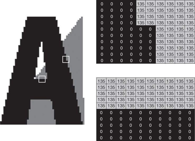
Figure 4.4
Nearest neighbor interpolation: interpolated image of “letter  ” and intensity maps of the enclosed diagonal and vertical edges.

Figure 4.5 Nearest neighbor interpolation of natural image Cat by a factor of 2 (PSNR = 25.98 dB): (a) the full interpolated image, (b) zoom‐in portion of cat's whiskers in original image, and (c) zoom‐in portion of cat's whiskers in interpolated image.
4.1.3 Bilinear
Bilinear interpolation is another well‐received interpolation technique because of its simplicity while it applies a better low‐pass filtering operation in the reconstruction that reduces the awkward jaggy artifact as perceived in the nearest neighbor interpolation. It should be noted that “bilinear” comes from the word “linear” with the prefix “bi‐,” which implies that the interpolation is in fact two linear operations. Bilinear interpolation is equivalent to the approximation of a straight line (linear interpolation) along row, followed by approximating a straight line (another linear interpolation) along column. Therefore, we can simplify our analytical discussion by considering the 1D linear interpolation kernel. Here shown is the interpolation kernel of the linear interpolation

The impulse response of this linear filter is shown in Figure 4.6 a, which is a triangular function. It should be noted that this figure is plotted by considering the special case of even weighting from neighboring pixels due to the fixed spacing between neighboring pixels in the digital image, which will be further elaborated later. The triangular function has ![]() regularity (continuous but not differentiable). It corresponds to a modest low‐pass filter in the frequency domain. Similar to all linear convolution image interpolation techniques, resampling operation comes first to generate the intermediate signal
regularity (continuous but not differentiable). It corresponds to a modest low‐pass filter in the frequency domain. Similar to all linear convolution image interpolation techniques, resampling operation comes first to generate the intermediate signal ![]()

However the interpolation result ![]() is obtained by convolving the filter in Eq. (4.10 ) to
is obtained by convolving the filter in Eq. (4.10 ) to ![]() . Hence, the interpolated result is given by
. Hence, the interpolated result is given by
where ![]() is a weighted sum of the two neighboring pixels with weighting factors
is a weighted sum of the two neighboring pixels with weighting factors ![]() on pixel
on pixel ![]() and
and ![]() on
on ![]() . In general case,
. In general case, ![]() is determined by the impact of the neighboring pixels toward the pixel under investigation or simply determined by the relative spacing of the two neighboring pixels to the pixel under investigation.
is determined by the impact of the neighboring pixels toward the pixel under investigation or simply determined by the relative spacing of the two neighboring pixels to the pixel under investigation.
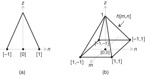
Figure 4.6 The plot of (a) linear interpolation kernel and (b) bilinear interpolation kernel in spatial domain.
The 1D linear interpolation can be easily extended to 2D and is known as the bilinear interpolation with the impulse response shown in Figure 4.6 b. The bilinear interpolation computes the pixel intensity of a pixel ![]() located at spatial coordinate
located at spatial coordinate ![]() by first locating the four corner pixels of the smallest box that surround
by first locating the four corner pixels of the smallest box that surround ![]() as shown in Figure 4.7 . These four coordinates can be extracted by the MATLAB code
as shown in Figure 4.7 . These four coordinates can be extracted by the MATLAB code
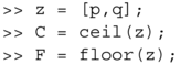
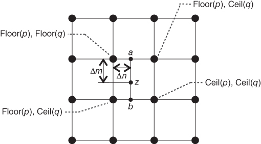
Figure 4.7
Spatial weighting map of the bilinear interpolation for the pixel  located at
  .
.
such that the four corner pixels are given by f(F(1):C(1), F(2):C(2)). The bilinear interpolation weighting to be assigned to each corner pixel is computed as the distance between ![]() and each corner pixel as given by the MATLAB code
and each corner pixel as given by the MATLAB code
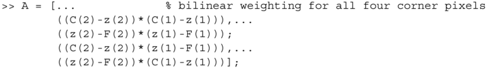
The interpolated pixel intensity b is given as the weighted sum of corner pixels:
![]()
It should be noted that if either p or q is integer, the above matrix A will be a zero matrix. Therefore, the case of integer p or q should be treated separately. In fact, if both p and q are integers, the interpolated pixel b should be equal to the pixel f(p,q). If either p or q is integer, but not both, linear interpolation on the axis that contains the non‐integer coordinate should replace the bilinear interpolation. In the case when q is not an integer,

If it is, p being not an integer,

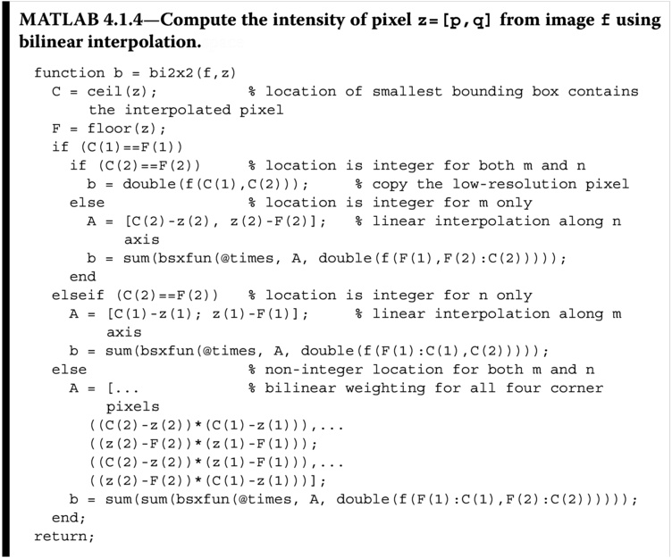
The MATLAB function bi2x2 listed in Listing 4.1.4 implements the above per‐pixel bilinear interpolation with a given image f and interpolated pixel location z=[p,q] and returns the intensity of the interpolated pixel.
The bilinear image interpolation with ratio r can be obtained by first generating the grid map of the interpolated image and then applying bi2x2 to compute the intensity of each pixel.
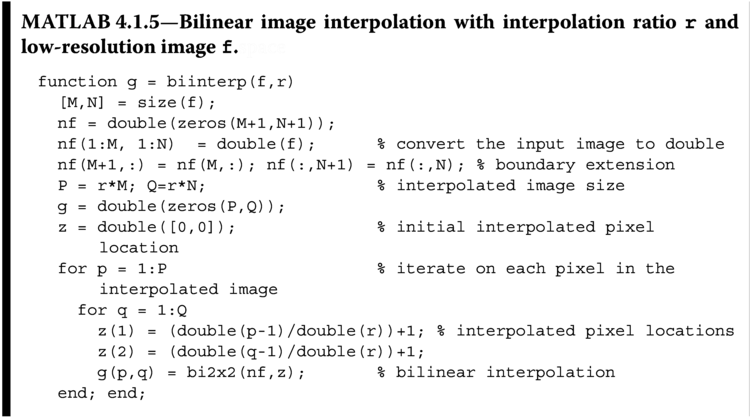
Noted that the image f has to be boundary extended (by adding one column at the rightmost and one row at the bottom) to accommodate the bilinear interpolation around boundary pixels. Among various extension methods, Listing 4.1.5 has implemented the infinite extension (boundary pixel value repetition) as discussed in Section 2.4.1.4. The bilinear interpolation result of the synthetic image letter A with interpolation ratio equal to 2 obtained from the MATLAB function call g=biinterp(f,2) is shown in Figure 4.8 where the intensity map along the horizontal edge and diagonal edge is also shown in the same figure. The staircase‐like artifact along the diagonal edge, which is also known as the jaggy artifact, is found to be the most severe artifact in nearest neighbor interpolation. The same artifact is also observed in bilinear interpolated natural image in Figure 4.8 . However, almost all edges are blurred in the interpolated letter A. Besides blurring, there is a ghost edge surrounding all edges of the letter A. Figure 4.9 shows the bilinear interpolated natural image Cat (see Figure 4.9 a). The interpolated image has a PSNR of 28.39 dB. The visual quality is pleasant around the texture‐rich region (Cat's forehead) of the interpolated image. However, there is serious jaggy along long edges (Cat's whiskers and hairs). The jaggy can be easily observed when compared with the zoom‐in (enclosed in boxes) of both the original image (see Figure 4.9 b,d) and the bilinear interpolated image (see Figure 4.9 c,e).
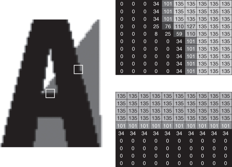
Figure 4.8
Bilinear interpolation: interpolated image of “letter  ” and intensity map of the enclosed diagonal and vertical edges.

Figure 4.9 Bilinear interpolation of natural image Cat by a factor of 2 (PSNR = 28.39 dB): (a) the full interpolated image, (b) zoom‐in portion of cat's whiskers in original image, (c) zoom‐in portion of cat's whiskers in interpolated image, (d) zoom‐in portion of cat's ear in original image, and (e) zoom‐in portion of cat's ear in interpolated image.
The averaging operation of the bilinear interpolation results in a smooth interpolated image when compared with that obtained from the nearest neighbor interpolation. The visual quality of the bilinear interpolated image is better than that of the nearest neighbor interpolated image with less jaggies, which are smoothed out by the averaging operation of the bilinear interpolation. In addition to the better visual quality, there is a substantially better objective quality obtained by the bilinear interpolated image. The PSNR of bilinear interpolated image is better than that of the nearest neighbor interpolated image. However, bilinear interpolated images suffer from severe blurring artifacts when compared with that of the nearest neighbor interpolated images. Furthermore, bilinear interpolation requires relatively higher computations when compared with that of the nearest neighbor interpolation algorithm.
4.1.4 Bicubic
Bicubic interpolation improves the bilinear interpolation by using a bigger interpolation kernel. The kernel size of the bicubic interpolation is ![]() as shown in Figure 4.10 , compared with the
as shown in Figure 4.10 , compared with the ![]() kernel of bilinear interpolation. As a result, bicubic interpolation is a third‐order interpolation, compared with the first‐order interpolation of bilinear interpolation and zero‐order interpolation of the nearest neighbor interpolation. The higher‐order interpolation can achieve interpolated image with sharper edges than that produced by bilinear interpolation, and at the same time it provides better suppression on jaggy artifacts when compared with that produced by nearest neighbor interpolation. However, the bicubic interpolation requires very complicated calculations. After all, the interpolation kernel is four times larger than that of bilinear interpolation.
kernel of bilinear interpolation. As a result, bicubic interpolation is a third‐order interpolation, compared with the first‐order interpolation of bilinear interpolation and zero‐order interpolation of the nearest neighbor interpolation. The higher‐order interpolation can achieve interpolated image with sharper edges than that produced by bilinear interpolation, and at the same time it provides better suppression on jaggy artifacts when compared with that produced by nearest neighbor interpolation. However, the bicubic interpolation requires very complicated calculations. After all, the interpolation kernel is four times larger than that of bilinear interpolation.

Figure 4.10 Bicubic interpolation: estimation of unknown pixels lying on the exact surface defined by the neighboring 16 pixels. (For color interpretation please refer the digital version of this figure.)
Similar to bilinear interpolation, the prefix “bi‐” of bicubic interpolation reveals its separability nature, where bicubic image interpolation can be implemented by sequential application of the 1D cubic spline interpolations along the row and then the column of the image. Consider the example in Figure 4.10 , where the original image lattice is expanded with up‐sampling ratio of 2. The black dots in Figure 4.10 illustrate the pixels preserved from the original image. The unknown pixels in between the original pixels have to be interpolated. We shall make use of the separable property of bicubic interpolation to compute the interpolated pixel value at ![]() from its neighboring original pixels. Therefore, we shall first compute four 1D cubic spline interpolations (the
from its neighboring original pixels. Therefore, we shall first compute four 1D cubic spline interpolations (the ![]() ,
, ![]() ,
, ![]() , and
, and ![]() functions plotted as dashed/red splines in the figure) to obtain the intermediate pixels
functions plotted as dashed/red splines in the figure) to obtain the intermediate pixels ![]() ,
, ![]() ,
, ![]() , and
, and ![]() (the white dots). These four intermediate pixels will be applied to another 1D cubic spline interpolation (the solid/blue splines in the figure) to produce the intensity of the unknown pixel
(the white dots). These four intermediate pixels will be applied to another 1D cubic spline interpolation (the solid/blue splines in the figure) to produce the intensity of the unknown pixel ![]() . As a result, we can complete the bicubic interpolation with a given 1D cubic spline interpolation kernel, which is generally defined as a combination of the piecewise cubic polynomials for the sake of simple implementation. Among various definitions of 1D cubic spline interpolation kernel, this book chooses the cubic spline interpolation given by Reichenbach and Geng [55 ] as shown in the following.
. As a result, we can complete the bicubic interpolation with a given 1D cubic spline interpolation kernel, which is generally defined as a combination of the piecewise cubic polynomials for the sake of simple implementation. Among various definitions of 1D cubic spline interpolation kernel, this book chooses the cubic spline interpolation given by Reichenbach and Geng [55 ] as shown in the following.

where ![]() is usually set in between the range of
is usually set in between the range of ![]() and
and ![]() . The piecewise cubic polynomials are nonzero with
. The piecewise cubic polynomials are nonzero with ![]() whatever the values of
whatever the values of ![]() , and this set of polynomials is also known as the basic function of cubic spline. The basic functions with
, and this set of polynomials is also known as the basic function of cubic spline. The basic functions with ![]() ,
, ![]() , and
, and ![]() are plotted in Figure 4.11 .
are plotted in Figure 4.11 .
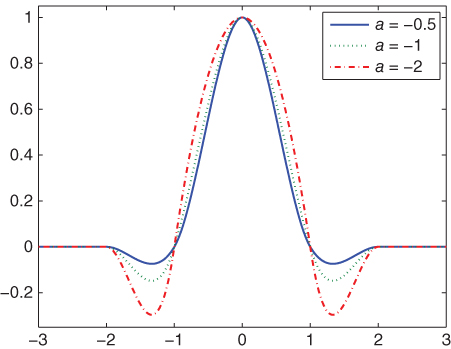
Figure 4.11 Basic function of cubic convolution.
The basic functions with different choices of ![]() show us that the smaller values of
show us that the smaller values of ![]() will result in an interpolation kernel with wider lobe, which is more helpful in preserving the image structure with greater feature size. The con is that its legs will go into more negative values that will result in more severe ringing artifacts in the interpolated image. Therefore, the quality of the interpolated image is highly dependent on the choice of
will result in an interpolation kernel with wider lobe, which is more helpful in preserving the image structure with greater feature size. The con is that its legs will go into more negative values that will result in more severe ringing artifacts in the interpolated image. Therefore, the quality of the interpolated image is highly dependent on the choice of ![]() . The best compromise is to choose
. The best compromise is to choose ![]() to be
to be ![]() , which forms the third‐degree cubic kernel [36 ]. Similar to the bilinear interpolation, the 1D cubic interpolation kernel can be extended to 2D version by convolution of the 1D filter to its transpose. Figure 4.12 shows the 2D plot of the impulse response of the bicubic interpolation kernel with
, which forms the third‐degree cubic kernel [36 ]. Similar to the bilinear interpolation, the 1D cubic interpolation kernel can be extended to 2D version by convolution of the 1D filter to its transpose. Figure 4.12 shows the 2D plot of the impulse response of the bicubic interpolation kernel with ![]() in spatial domain. Though the bicubic interpolation can be realized by the convolution of the 2D filter to the neighboring pixels for all pixels in the image, the computation is very exhaustive. Therefore, the practical implementation will usually make use of the separable property of the kernel and perform the interpolation as illustrated in Figure 4.10 with the 1D cubic spline interpolation kernel given by Eq. (4.13 ).
in spatial domain. Though the bicubic interpolation can be realized by the convolution of the 2D filter to the neighboring pixels for all pixels in the image, the computation is very exhaustive. Therefore, the practical implementation will usually make use of the separable property of the kernel and perform the interpolation as illustrated in Figure 4.10 with the 1D cubic spline interpolation kernel given by Eq. (4.13 ).

Figure 4.12 The 2D bicubic interpolation kernel in spatial domain.
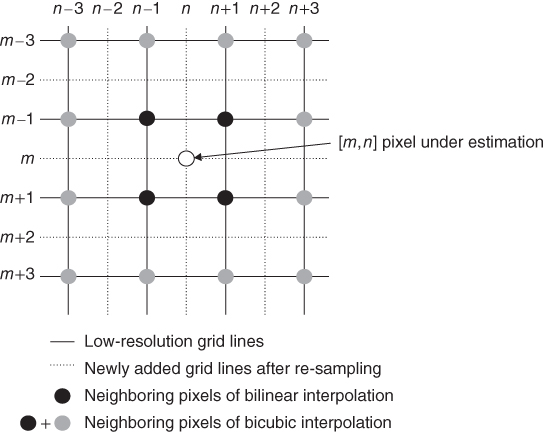
Figure 4.13 Neighboring pixels of bilinear and bicubic interpolation.
Before we go into the MATLAB implementation of the bicubic interpolation, it will be easier for the readers to get an idea on the collection of the neighboring pixels for bicubic interpolation and the major difference of such collection when compared with that of bilinear interpolation. Figure 4.13 shows part of the high‐resolution grid with pixel ![]() being the pixel under estimation (the white dot) to illustrate the relative location of the neighboring pixels to
being the pixel under estimation (the white dot) to illustrate the relative location of the neighboring pixels to ![]() . As described in Section 4.1.3 , we need four closest known pixels surrounding the pixel under estimation (the black dots at
. As described in Section 4.1.3 , we need four closest known pixels surrounding the pixel under estimation (the black dots at ![]() ,
, ![]() ,
, ![]() , and
, and ![]() ), where the known pixels are those pixels taken from the low‐resolution image. The unknown pixel
), where the known pixels are those pixels taken from the low‐resolution image. The unknown pixel ![]() is estimated as the weighted sum of the four neighboring pixels in bilinear interpolation. For bicubic interpolation, 12 additional numbers of neighboring pixels will be considered (the gray dots), such that the collection will contain both the black and gray pixels (
is estimated as the weighted sum of the four neighboring pixels in bilinear interpolation. For bicubic interpolation, 12 additional numbers of neighboring pixels will be considered (the gray dots), such that the collection will contain both the black and gray pixels (![]() with
with ![]() and
and ![]() ). In other words, we can name the kernel size
). In other words, we can name the kernel size ![]() and
and ![]() for bilinear interpolation and bicubic interpolation, respectively, where the dimensions 2 and 4 are equivalent to the number of low‐resolution pixels in row–column direction counted toward to the interpolation. It is vivid that the bicubic interpolation works with a bigger interpolation kernel, which will be beneficial to preserve image feature in greater size; however, the computation is more complicated. It should also be noted that the kernel size for both the bilinear and bicubic cases are extensible but the computation complexity will inevitably increase. Moreover, the blurring artifacts in bilinear interpolation with larger kernel size will be more significant.
for bilinear interpolation and bicubic interpolation, respectively, where the dimensions 2 and 4 are equivalent to the number of low‐resolution pixels in row–column direction counted toward to the interpolation. It is vivid that the bicubic interpolation works with a bigger interpolation kernel, which will be beneficial to preserve image feature in greater size; however, the computation is more complicated. It should also be noted that the kernel size for both the bilinear and bicubic cases are extensible but the computation complexity will inevitably increase. Moreover, the blurring artifacts in bilinear interpolation with larger kernel size will be more significant.
Listing 4.1.6 is the MATLAB bicubic interpolation function (bicubic(f,r)) that up‐samples an image f with interpolation ratio ![]() . The parameter
. The parameter gridSize is an array containing the relative position of the neighboring pixels (in the input image f) to be considered in the interpolation with reference to the position of the unknown pixel in the final image g. The gridSize further combines with the parameters di and dj to provide sufficient information to define all the required neighboring pixels, where di and dj are the distances of the unknown pixel relative to corresponding neighboring pixels in row and column directions, respectively. For the case of ![]() and with the grid size in digital image being even, the values of
and with the grid size in digital image being even, the values of di and dj are equal and are given by ![]() . Based on
. Based on gridSize, di, and dj, the neighboring pixels aX, bX, cX, dX, aY, bY, cY, and dY are obtained. This pixel location computation is essential in image interpolation because the operation involves resampling. The parameter afact defines the weighting factor ![]() in Eq. ( 4.13
), which will be used to estimate the unknown pixel.
in Eq. ( 4.13
), which will be used to estimate the unknown pixel.
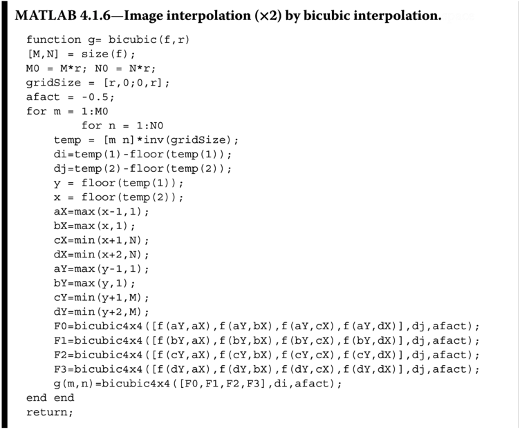
The program then calls another function bicubic4x4 given by MATLAB Listing 4.1.7, which is the realization of Eq. ( 4.13
) with the first parameter defining the v matrix containing the pixel intensities of the required pixels required in forming the bicubic function as shown in Eq. ( 4.13
), the second parameter defining the relative position to be estimated, and the third parameter defining the variable ![]() . It should be noted that the bicubic interpolation problem is also separable, such that the computation can be achieved by computing the 1D estimation along row and then along column. Hence, we can obtain
. It should be noted that the bicubic interpolation problem is also separable, such that the computation can be achieved by computing the 1D estimation along row and then along column. Hence, we can obtain F0, F1, F2, and F3 (![]() ,
, ![]() ,
, ![]() , and
, and ![]() as shown in Figure 4.10 ) and further apply these four functions to another
as shown in Figure 4.10 ) and further apply these four functions to another bicubic4x4 to give the value of the pixel in the final image g(i,j) (the unknown pixel in Figure 4.10 ).

Figure 4.14 shows the bicubic interpolation results on the synthetic image letter A with ![]() interpolation ratio by the MATLAB function call
interpolation ratio by the MATLAB function call g=bicubic(f,2), where the intensity maps along the horizontal edge and diagonal edge are also shown in the same figure. It is vivid that there are overshoots in pixel intensities when the interpolation is along two regions with extreme intensities (across edges). This artifact is known as overshooting and is observed to be multiple inverted paths parallel to edges. The same artifact is also observed in bicubic interpolated natural image, and this artifact distorts the image in the form of ringing as shown in the result of the bicubic interpolated natural image Cat (see Figure 4.15 a) with PSNR of 24.9 dB. To facilitate the discussion, the zoom‐in portions of the whiskers and ear of the original Cat image are shown in Figure 4.15 b,d, respectively, while the corresponding portions of the bicubic interpolated image are shown in Figure 4.15 c,e, respectively. It shows consistent performance at the texture‐rich region (forehead of the Cat image) as that of nearest neighbor interpolation and bilinear interpolation. The bicubic interpolation achieves better interpolation results along long edges (as shown in the whiskers of the Cat image in Figure 4.15 b,c) in order to preserve the edge sharpness when compared with that of bilinear interpolation. Moreover, the bicubic interpolation results in less blurred image around the ear of the Cat (see Figure 4.15 d,e) when compared with that of bilinear interpolation. These observations show that bicubic interpolation is able to preserve the image features due to the use of higher‐order function in the interpolation and also the use of larger interpolation kernel. However, the whiskers are turned to be zigzag‐like structure in the bicubic interpolated image that is attributed to the ringing artifacts and also because of the overshoot at the boundary of the ![]() kernels. Large intensity changes along sharp edges with overshoots generate unnatural appearance of bright and dark pixels along the two adjacent bicubic surfaces. Once such pattern repeats across several surfaces, it will be observed as the zigzag artifact. Nonetheless, bicubic interpolation results in the lowest PSNR value among nearest neighbor interpolation and bilinear interpolation due to the higher noise level encountered in the large kernel.
kernels. Large intensity changes along sharp edges with overshoots generate unnatural appearance of bright and dark pixels along the two adjacent bicubic surfaces. Once such pattern repeats across several surfaces, it will be observed as the zigzag artifact. Nonetheless, bicubic interpolation results in the lowest PSNR value among nearest neighbor interpolation and bilinear interpolation due to the higher noise level encountered in the large kernel.

Figure 4.14
Bicubic interpolation: interpolated image of “letter  ” and intensity maps of the enclosed diagonal and vertical edges.

Figure 4.15 Bicubic interpolation of natural image Cat by a factor of 2 (PSNR = 24.9 dB): (a) the full interpolated image, (b) zoom‐in portion of Cat's whiskers in original image, (c) zoom‐in portion of Cat's whiskers in interpolated image, (d) zoom‐in portion of Cat's ear in original image, and (e) zoom‐in portion of Cat's ear in interpolated image.
In general, bicubic interpolation generates better visual quality than bilinear interpolation. For smooth regions, bicubic interpolation generates smoother outputs because the derivatives across source pixels on a surface generated by bicubic polynomials are continuous but the ones by bilinear polynomials are not. For edges, bicubic polynomials generate overshoots that enhance contrast and are visually favorable because most high quality natural images contain visually sharp edges.
4.2 Frequency Domain Analysis
In Section 4.1 , we have focused our discussions on the three basic nonadaptive interpolation methods in the spatial domain, where their interpolation kernels have also been introduced. The interpolation methods in Section 4.1 can be interpreted as 2D filtering zero‐padded up‐sampled images by 2D filters formed by the interpolation kernels. Knowing that it is a filtering operation, the interpolation problem can therefore be analyzed in the frequency domain, such as to reveal the properties of each interpolation method through the frequency response of the interpolation kernels.
To simplify the discussions, we shall state the frequency response of the interpolation kernel of the nearest neighbor interpolation, bilinear interpolation, and bicubic interpolation below, without going through the step‐by‐step computation of Fourier transform of these kernels. The readers can go through the derivation on their own with reference to Section 2.3.
The frequency responses of the sinc function (![]() ), the nearest neighbor interpolation kernel (
), the nearest neighbor interpolation kernel (![]() ), the bilinear interpolation kernel (
), the bilinear interpolation kernel (![]() ), and the bicubic interpolation kernel (
), and the bicubic interpolation kernel (![]() ) are given by
) are given by

where ![]() is the bandwidth of the sinc function. It should be noted that due to the separable property of these four interpolation filters, only the 1D frequency responses will be presented and discussed. The spatial and frequency responses of the above four filters are plotted in Figure 4.16 .
is the bandwidth of the sinc function. It should be noted that due to the separable property of these four interpolation filters, only the 1D frequency responses will be presented and discussed. The spatial and frequency responses of the above four filters are plotted in Figure 4.16 .

Figure 4.16 The spatial (a) and frequency response (b) of the nearest neighbor, bilinear, and bicubic interpolation kernels. (See insert for color representation of this figure.)
There are two things of interest for the design of reconstruction filter: the passband and the stopband. The passband governs which portion of the frequency components can be retained after the reconstruction, while the stopband suppresses the unwanted frequency components so they will not be appeared in the reconstructed signal. In ideal case, perfect reconstruction requires a low‐pass filter with passband greater than all the frequency components that needed to be preserved. Therefore, as shown in Figure 4.16 , only the sinc filter is the most appropriate candidate for perfect reconstruction as it has a sharp cutoff at ![]() . However, it is not practical to implement this filter in real application because it is not possible to implement infinite number of samples in spatial domain to preserve the perfect sinc function. The nearest neighbor filter, bilinear filter, and bicubic filter that have the same cutoff frequency at
. However, it is not practical to implement this filter in real application because it is not possible to implement infinite number of samples in spatial domain to preserve the perfect sinc function. The nearest neighbor filter, bilinear filter, and bicubic filter that have the same cutoff frequency at ![]() are shown in the same figure. The nearest neighbor filter has a relatively steeper falloff, and it can achieve better reconstruction, where more high frequency components (close to
are shown in the same figure. The nearest neighbor filter has a relatively steeper falloff, and it can achieve better reconstruction, where more high frequency components (close to ![]() ) can be preserved, such that the final image will be sharper. However, it has many subharmonic lobes such that the high frequency components falling in those lobes will appear in the reconstructed image. As a result, severe jaggy artifacts are observed in the interpolation results. The bilinear filter has a degraded passband that suppresses some of the high frequency components in the image, thus resulting in a blurred image. However, its subharmonic lobes have lower magnitudes; thus the jaggy artifacts are less severe when compared with that of nearest neighbor filter. The con is that the bilinear filter interpolated images show more severe ringing artifacts. The bicubic filter has a similar passband as that of bilinear filter, while it has even weaker subharmonic lobes that help to further suppress the effect of unwanted high frequency components in the interpolated images. The interpolated images are observed to be similar to that obtained with the application of bilinear filter but with improvement in the suppression of ringing artifacts.
) can be preserved, such that the final image will be sharper. However, it has many subharmonic lobes such that the high frequency components falling in those lobes will appear in the reconstructed image. As a result, severe jaggy artifacts are observed in the interpolation results. The bilinear filter has a degraded passband that suppresses some of the high frequency components in the image, thus resulting in a blurred image. However, its subharmonic lobes have lower magnitudes; thus the jaggy artifacts are less severe when compared with that of nearest neighbor filter. The con is that the bilinear filter interpolated images show more severe ringing artifacts. The bicubic filter has a similar passband as that of bilinear filter, while it has even weaker subharmonic lobes that help to further suppress the effect of unwanted high frequency components in the interpolated images. The interpolated images are observed to be similar to that obtained with the application of bilinear filter but with improvement in the suppression of ringing artifacts.
4.3 Mystery of Order
We have discussed first‐order, second‐order, and third‐order polynomial interpolation methods with the nearest neighbor interpolation, bilinear interpolation, and bicubic interpolation, respectively. It is possible to further increase the interpolation filter kernel to higher order to improve the interpolation quality. Mathematically, a 1D ![]() th‐order polynomial interpolation kernel can be applied to perfectly interpolate
th‐order polynomial interpolation kernel can be applied to perfectly interpolate ![]() data points, such that the interpolated curve is smooth and it passes through all the data points. However, the application of higher‐order polynomial interpolation kernel to the entire dataset with unlimited bandwidth will lead to unwanted artifacts, including overshoot and oscillation around pixels with abrupt intensity changes as illustrated in Figure 4.17 .
data points, such that the interpolated curve is smooth and it passes through all the data points. However, the application of higher‐order polynomial interpolation kernel to the entire dataset with unlimited bandwidth will lead to unwanted artifacts, including overshoot and oscillation around pixels with abrupt intensity changes as illustrated in Figure 4.17 .
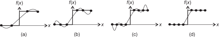
Figure 4.17
A visual representation of a situation where linear interpolation is superior to higher‐order interpolating polynomials. The function to be fit (an edge) undergoes an abrupt change at  . Parts (a)–(c) indicate that the abrupt change induces oscillations in interpolating polynomials. In contrast, because it is limited to third‐order curves with smooth transitions, a linear interpolation (d) provides a much more acceptable approximation.

Figure 4.18 Illustration of different spline functions: (a) first‐order spline, (b) second‐order spline, and (c) cubic spline.
The number of data points considered in the interpolation is increased from 4 in Figure 4.17 a to 8 in Figure 4.17 c, which improves the approximation. The increase in the data points considered is actually increasing the order of the polynomial interpolation kernel. However, increasing the polynomial order will result in overshoot and oscillation around pixels (as shown in Figure 4.17 c), which degrades the interpolation performance. To reduce the overshoot and oscillation artifacts in image interpolation, practical image interpolation makes use of piecewise continuous interpolation (as shown in Figure 4.17 d). Consider the case of piecewise continuous interpolation by spline functions with various orders. The lowest‐order spline function is the first‐order spline, which is also known as the linear spline. The linear spline connects all data points using a series of linear lines. The linear spline itself is continuous, but its first derivative is not continuous (see Figure 4.18 a). It is vivid that the interpolation result is not satisfactory, where the first‐order approximation is not detailed enough to estimate the smooth curve. When we increase the spline function order to 2, where the spline function is known as the spline of degree 2 or second‐order spline, the spline function itself and its first derivatives are continuous throughout all data points under consideration. Moreover, the spline function has to be a polynomial of degree at most 2 on each subinterval formed by two consecutive points inside the entire interval under consideration. In other words, the second‐order spline is a quadratic spline that is continuously differentiable piecewise quadratic function. The second‐order spline interpolation result is shown in Figure 4.18 b. We can observe that the second‐order spline generates a more pleasant interpolation result when compared with that of linear spline. If we further increase the order of the spline function to 3, which is known as spline of degree 3 or third‐order spline, the third‐order spline has continuous first derivative and second‐order derivatives over the entire interval under consideration. Moreover, the functions in the subintervals formed by two consecutive data points also described by a polynomial of degree at most 3 over the entire data set. It can be observed from Figure 4.18 c that the third‐order spline generates the best interpolation result among that obtained by interpolation using the linear and quadratic spline functions. The third‐order spline is known as the cubic spline, which overcomes the problem of “overshoot,” and it is easier to deal with when compared with that of higher‐order polynomials. Extensive research works have showed that further increasing the spline function order does not provide further improvement in the quality of the interpolated image, while the complexity of the interpolation using high‐order kernel is exponentially increasing with respect to the kernel size, which is defined by the spline function order. In other words, the high‐order spline functions have prohibitively high computational complexity to prevent them from applying in practical cases. At the same time, we should also note that the spline function has improved smoothness with increasing spline function order. This is caused by both the large kernel size and the continuity of high‐order derivative. Therefore, application of high‐order spline function for image interpolation with spline function order higher than 3 can seldom be found in real‐world applications. Extensive research works have shown that the cubic spline is almost the best one to obtain the best interpolation among all spline function orders.

Figure 4.19 Example of affine transformation: (a) input image and (b) transformed image.
4.4 Application: Affine Transformation
The above nonparametric interpolation techniques are commonly used in image processing applications, either being invoked alone or being applied with other image processing techniques. In this section, we shall discuss one of the applications of image interpolation to affine transformation, which we have briefly introduced in Section 2.6. Affine transformation of an object is the general form of all geometric transformations, which is the operation of series of geometric transformation, including translation, rotation, and scaling. Affine transformation maps an object from one coordinate system to another system, where the shape of the object may not be maintained, but the transformation will maintain:
- Straight line to be straight.
- Parallel lines to be parallel.
- Midpoint of a line to be the midpoint of the transformed line.
Affine transformation is a particular form of the geometric transformation. Let us recall the general geometric transformation formula depicted in Eq. (2.55).
where ![]() and
and ![]() can be the concatenation or multiplication of the transformation matrices discussed in Section 2.6. In other words, translation, rotation, and scaling are the three most simple and independent cases of the affine transformation, and the sequence of transformations would affect the structure of
can be the concatenation or multiplication of the transformation matrices discussed in Section 2.6. In other words, translation, rotation, and scaling are the three most simple and independent cases of the affine transformation, and the sequence of transformations would affect the structure of ![]() and
and ![]() due to the concatenation or multiplication of matrix operations. Figure 4.19 shows one of the practical application of affine transform, which rectifies an alphabet to regular alignment for the ease of reading. The tilted alphabet (shown in Figure 4.19 a) can be due to the misalignment of the object to the capturing device, commonly seen in document scanning application. The four vertices in Figure 4.19 a forms
due to the concatenation or multiplication of matrix operations. Figure 4.19 shows one of the practical application of affine transform, which rectifies an alphabet to regular alignment for the ease of reading. The tilted alphabet (shown in Figure 4.19 a) can be due to the misalignment of the object to the capturing device, commonly seen in document scanning application. The four vertices in Figure 4.19 a forms ![]() in Eq. (4.18 ). The matrices
in Eq. (4.18 ). The matrices ![]() and
and ![]() map the points in
map the points in ![]() to give
to give ![]() in Figure 4.19 b. It is vivid that the irregular image has been rotated and scaled such that the entire image can be fully fitted onto the predefined rectangular frame, where the shape of the original image and final image are different but all straight lines remain straight and parallel lines remain in parallel. Unfortunately, the mapping of pixel coordinates may not necessarily produce output coordinates in integer. Hence, round off on the output coordinates is inevitable. On the other hand, the display system, printing system, and standard image storage system can only handle images defined in an integer Cartesian coordinate system. As a result, there will be missing pixels in the final image, where image interpolation steps in to estimate the unknown pixel values. The importance of image interpolation in affine transformation can be more easily observed by considering one of its special case, image rotation, as illustrated in Figure 4.20 .
in Figure 4.19 b. It is vivid that the irregular image has been rotated and scaled such that the entire image can be fully fitted onto the predefined rectangular frame, where the shape of the original image and final image are different but all straight lines remain straight and parallel lines remain in parallel. Unfortunately, the mapping of pixel coordinates may not necessarily produce output coordinates in integer. Hence, round off on the output coordinates is inevitable. On the other hand, the display system, printing system, and standard image storage system can only handle images defined in an integer Cartesian coordinate system. As a result, there will be missing pixels in the final image, where image interpolation steps in to estimate the unknown pixel values. The importance of image interpolation in affine transformation can be more easily observed by considering one of its special case, image rotation, as illustrated in Figure 4.20 .

Figure 4.20 Image rotation through pixel mapping from original coordinate grid to a rotated grid: (a) rotated Cat image, (b) missing pixel after rotation, and (c) illustration of pixel mapping in image rotation.
Rotating an image is a simple affine mapping that remaps the image pixels from one position (the original image Cartesian coordinate ![]() ) to a new position (the rotated coordinate
) to a new position (the rotated coordinate ![]() ). They are related by affine transform equation with the rotation angle
). They are related by affine transform equation with the rotation angle ![]() as parameter with the geometric transformation matrix given by Eq. (2.69) for clockwise rotation with
as parameter with the geometric transformation matrix given by Eq. (2.69) for clockwise rotation with ![]() being positive and restated in the following again.
being positive and restated in the following again.

Since image coordinates can only be discrete values, some transformations resulting from integer ![]() may require either
may require either ![]() or
or ![]() in
in ![]() to be non‐integer. As a result, some of the pixels of the rotated image cannot be mapped to a pixel in the original image. An example of the Cat image being rotated by
to be non‐integer. As a result, some of the pixels of the rotated image cannot be mapped to a pixel in the original image. An example of the Cat image being rotated by ![]() is shown in Figure 4.20 a. When we zoom into a small box within the image as shown in Figure 4.20 b, there are numbers of missing pixels that correspond to the coordinates
is shown in Figure 4.20 a. When we zoom into a small box within the image as shown in Figure 4.20 b, there are numbers of missing pixels that correspond to the coordinates ![]() that maps to a non‐integer coordinate
that maps to a non‐integer coordinate ![]() . To demonstrate this remapping problem graphically, let us consider Figure 4.20 c. The rotation makes reference to a chosen origin, the reference pixel, which in our case is the black dot. Rotation moves the pixels to new locations by mapping the original pixels to a new coordinate system. However, the mapping is determinative, and there will be overlapping or skipping in the new system. As a result, the remapping will sometimes result with pixels having no value assigned to them in the new system and sometimes with more than one pixel from the original image to be contributed to the rotated image. The artifacts are more severe along the image boundary.
. To demonstrate this remapping problem graphically, let us consider Figure 4.20 c. The rotation makes reference to a chosen origin, the reference pixel, which in our case is the black dot. Rotation moves the pixels to new locations by mapping the original pixels to a new coordinate system. However, the mapping is determinative, and there will be overlapping or skipping in the new system. As a result, the remapping will sometimes result with pixels having no value assigned to them in the new system and sometimes with more than one pixel from the original image to be contributed to the rotated image. The artifacts are more severe along the image boundary.
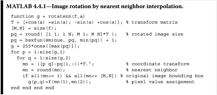
To avoid and suppress the artifacts aroused after the coordinate transformation, interpolation technique is applied to estimate and assign pixel values to the rotated image. As discussed in this chapter, there are a number of interpolation techniques that we can make use of. First, let us consider the nearest neighbor interpolation, such as to introduce the detailed implementation on how to rotate a digital image in the most simple manner. The following Listing 4.4.1 implements rotatenn that rotates the image f with radian angle a using nearest neighbor interpolation.
To obtain the ![]() rotated Cat image, we shall invoke
rotated Cat image, we shall invoke rotatenn as

The nearest neighbor interpolation is being performed by substituting the pixels that map to non‐integer spatial coordinates in the original image with pixel values in the location obtained by rounding of the pixel coordinates, which in strict sense is not nearest neighbor, but this implementation gives a close enough nearest neighbor interpolation result to demonstrate the mapping of pixel values in two coordinate systems. This algorithm can be easily improved to use bilinear interpolation for improved image quality as demonstrated by Listing 4.4.2.

A ![]() rotated Cat image using
rotated Cat image using rotatebi is shown in Figure 4.21 b. Shown in the same Figure 4.21 a is the Cat image obtained from rotatenn by nearest neighbor interpolation. It can be observed that the rotated image obtained from nearest neighbor interpolation is blocky, just like that of the interpolated image obtained from nearest neighbor interpolation. But the rotated image obtained from bilinear interpolation has better image quality. It can be conjectured that for better image interpolation algorithm can produce rotated image with better image quality.
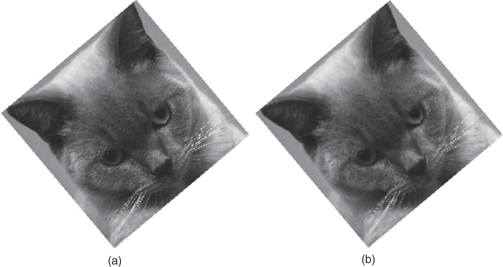
Figure 4.21
Cat image rotated with  obtained from (a) nearest neighbor interpolation by
 rotatenn(f,a) with f being the Cat image matrix and  and (b) bilinear interpolation by
 rotatebi(f,a).

Figure 4.22
Image interpolation algorithm structural integrity evaluation by considering the image rotated 9 times with angle  for (a) nearest neighbor, (b) bilinear, and (c) bicubic.
4.4.1 Structural Integrity
There is no accident for us to discuss the application of image interpolation to image rotation in this chapter. It is our intention to use image rotation to demonstrate the importance of the structural quality factor to image interpolation algorithm, which is something that cannot be measured by PSNR or SSIM. As discussed in previous section, image rotation requires to resample an image from a square lattice to another lattice grid that describes the rotated image. This is a lossy operation except for some special angle of rotation. The amount and quality of information loss will depend on the image interpolation method being applied in the resampling process since information lost in the rotation operation is accumulative. As a result, it can be expected that the image will be largely distorted after the image goes through successive rotations. The image interpolation method that obtains the best rotated image is also known as the one that can best preserve the structure of the image. It is not scientific to use the word “best” without an analytical metric to define the quality of the rotation, because the only information that we have is the original image ![]() before rotation. We can therefore define a rotation quality metric using the PSNR quantity between the given image
before rotation. We can therefore define a rotation quality metric using the PSNR quantity between the given image ![]() and the image obtained by nine successive rotations of
and the image obtained by nine successive rotations of ![]() or radian angle of
or radian angle of ![]() on the image
on the image ![]() . It is understood that the intermediate rotated image will have larger support and the final rotated image will be cropped to the initial image size. Figure 4.22 shows the above described procedure.
. It is understood that the intermediate rotated image will have larger support and the final rotated image will be cropped to the initial image size. Figure 4.22 shows the above described procedure.
Besides the rotation functions implemented in previous section, MATLAB image processing toolbox has a built‐in image rotation function imrotate(f,a,method), where method specifies the interpolation method to be applied to recover the pixels mapped to non‐integer coordinates during rotation. The available interpolation methods include nearest for nearest neighbor interpolation discussed in Section 4.1.2 , bilinear for bilinear interpolation discussed in Section 4.1.3 , and bicubic for bicubic interpolation discussed in Section 4.1.4 . The rotated images using imrotate after nine successive rotations of ![]() as shown in Figure 4.22 are shown at the bottom of Figure 4.22 , with the PSNR and SSIM of the resulting images obtained by different interpolation methods listed in Table 4.1 .
as shown in Figure 4.22 are shown at the bottom of Figure 4.22 , with the PSNR and SSIM of the resulting images obtained by different interpolation methods listed in Table 4.1 .
Table 4.1 PSNR and SSIM of Cat image down‐sampled to ![]() and rotated 9 times with angle
and rotated 9 times with angle ![]() .
.
| Nearest | |||
| neighbor | Bilinear | Bicubic | |
| PSNR (dB) | 22.7552 | 25.5519 | 28.0559 |
| SSIM | 0.6305 | 0.7280 | 0.8501 |
Performing the rotation using nearest neighbor interpolation clearly provides a poor quality as shown in Figure 4.22 a. The bilinear interpolation‐based rotation provides blurred images in Figure 4.22 b. The bicubic interpolation‐based rotation outperformed the other two, and the generated image closely resembles the image structure of the original image as shown in Figure 4.22 c. Readers may argue that the performance of different interpolation methods can be compared through studying of the PSNR and SSIM of the interpolated images as presented in previous sections. It may be true that the PSNR and SSIM can provide us some insight on the structural integrity of the interpolation algorithm. However, the small differences in the numeric values of PSNR and SSIM between various interpolation methods do not translate to such a large structural integrity difference as that revealed through image rotations as shown in Figure 4.22 and Table 4.1 . The ability to demonstrate the preservation of structural integrity is the reason why image rotations have been adapted in some literature to investigate and compare the performance of image interpolation methods.
4.5 Summary
In this chapter, we have started our journey in the exploration of different image interpolation methods by first investigating the nonparametric image interpolation methods. Down to the application level, image interpolation is the process of enlarging or expanding the size of an image. The size of the image can be enlarged due to the resample and reconstruction of the image by a particular image interpolation process. The resample step expands the resolution of the original images by increasing the sampling rate of the image in both the row and column directions, which is usually accomplished by inserting new zeros in between the pixels in the original image in spatial domain or duplicating the image spectrum in frequency domain (as will be discussed in Chapter 5). The reconstruction step estimates the intensities of pixels located at those newly inserted zero value spatial locations during the resampling step, where the estimation can also be completed by a convolution operation with the interpolation kernel. Most practical interpolation kernels are low‐pass in nature. It is vivid in frequency domain that such resampling and reconstruction do not introduce new information to the final image; however, the quality of the low‐pass filter does affect the quality of the final image. The nature of the low‐pass filter is therefore the key topic to be considered in this chapter and also in the later chapters. We have reviewed the properties of the interpolation kernel in spatial domain, and the reason why we have been focused in the spatial domain is because most of the implementation of image interpolation algorithms is in spatial domain. Among the many interpolation kernels, we have gone through the three most basic linear spatially invariant interpolation kernels, also known as the nonparametric interpolation kernels (because the filter does not depend on the image nature). The three interpolation methods are the nearest neighbor interpolation, bilinear interpolation, and bicubic interpolation. The discussions on each interpolation method cover the description of the interpolation filters of each method in both spatial and frequency domains. To facilitate analysis and implementation, their spatial matrix representations are also discussed. MATLAB source codes of each method are presented with detailed discussions to connect the source codes to the mathematical derivations. The performance of each method is compared with both the subjective (mainly concerns about the visual artifacts: blurring, jaggy, blocking, etc.) and objective (PSNR and SSIM) measures. The nearest neighbor interpolation is the replication of neighboring known pixel value to the unknown pixels, which makes use of a box‐shaped filter. This method has the simplest computation, but it suffers from severe staircase‐like artifacts (jaggies) along the region with sharp contrast changes (edges). Bilinear interpolation tends to produce interpolated images that appear softer, where the contrast is reduced because of the averaging of neighboring pixel values through the convolution of a triangular‐shaped filter in spatial domain. Improved quality interpolated image can be obtained from bicubic interpolation when compared with that of the nearest neighbor interpolation and bilinear interpolation. Bicubic interpolation makes use of third‐order approximation to achieve better reconstruction, especially along regions with sharp contrast changes. Therefore, the interpolated image obtained by bicubic interpolation preserves the advantage of bilinear interpolation and also provides more visually pleasant results along the high contrast region. However, the kernel of bicubic filter is a high‐order filter kernel that may result in overshooting (also known as ringing), thus degrading the PSNR performance.
Besides spatial domain analysis, in‐depth comparison of these three filters is also performed in the frequency domain, where the frequency response of each filter is presented. The passband and the stopband of the filter govern which frequency components can be preserved and which to be discarded during the reconstruction process. We also investigate the effect of estimation order. Though increasing the estimation order can reduce the estimation error, however, the interpolated image will suffer from overshooting and undergoing artifacts near the abrupt change regions. As a result, the optimal order of the interpolation filter kernel will be 3 for most practical image interpolation applications with natural images. Finally, we conclude this chapter's discussion on nonparametric interpolation filter by applying the interpolation in affine transformation and pointing out the importance of preserving the structure properties of the interpolated image. In the following chapters, we shall go through more advanced interpolation methods, where the image nature will be considered during the interpolation to achieve better interpolated image quality.
4.6 Exercises
- 4.1
Derive a causal interpolation filter kernel for the nearest neighbor and bilinear interpolations and implement the filter kernels in MATLAB. Analyze and discuss the following.
- The consequence of implementing the filter kernel in MATLAB when compared with the corresponding filter kernel discussed in this chapter
- The difference in the boundary extension required for the noncausal filters and that of the corresponding filter kernel discussed in this chapter to achieve signal interpolation
- 4.2
Given the following pixel values
 , use bilinear interpolation to estimate the pixel value at location
  .
(4.20)
.
(4.20)
- 4.3
With reference to Listing 4.1.3, develop a MATLAB function
nn(f,k), that will return a nearest neighbor interpolated image of ratiok, wherek .
. - 4.4
With reference to Listing 4.1.6, develop a MATLAB function
cubicspline6(f,k), that will return an order 3 (with kernel size ) cubic spline interpolated image of ratio
 k, wherek .
. - 4.5
[Affine transformation] Write a MATLAB code for computing an affine transform with a given image. The inputs to your program are (i) image, (ii) parameters of the affine transform, and (iii) interpolation method. Your report should include:
- M‐file with a well‐commented code.
- The result, namely,
 , when the input image is spatially transformed using the matrix
  and the bilinear interpolation, where
  is specified as
(4.21)
is specified as
(4.21)
- The difference between the input image and the image that has been obtained by applying the inverse spatial transform
 to
to  (apply zero padding if the images have different sizes). Explain the meaning of bright and dark pixels.
(Hint: MATLAB commands: “maketform,” “imtransform.”) - 4.6 [Frequency domain image rotation and shear] Rotation and shear are just special cases of affine transformation. As the component shears can be chosen to be purely in the
 and
and  directions, a rotation can be split into three one‐dimensional operations. The process is most clearly defined in terms of a matrix equation as
(4.22)
directions, a rotation can be split into three one‐dimensional operations. The process is most clearly defined in terms of a matrix equation as
(4.22)
where
 is the original image coordinate and
  is the mapped coordinate of the rotated image with clockwise rotation angle
  . The three component shears are as follows(4.23)
with the shearing transforms
(4.24)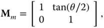 (4.25)
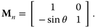
A simple application of the Fourier shift theorem will be equivalent to a one‐dimensional B‐spline interpolation. The following is a particular implementation to perform shearing of image
fin direction with
  :
:
Performing the above operation will generate a sheared image
fm. Complete the rest of the MATLAB source to perform Eq. (4.23 ) and generate a rotated image offwith clockwise rotation of .
. - 4.7 [Color demosaic]
- Develop a MATLAB function that read in full‐color image matrices, such as that of the full‐color Cat image, and output a Bayer pattern encoded color image matrix as shown in Figure 2.28. Plot the overlay image.
- Develop an image interpolation function that will read in the Bayer pattern encoded image matrix, and interpolate the matrix to obtain three separate full‐color image matrices. Plot the demosaic color image.
- Explain your choice of interpolation method in the above demosaic function. What are the pros and cons of using the selected interpolation method. Use demosaic image result to sustain your discussions.
- 4.8
Expand the sequence below to lengths of (i) 9, (ii) 11, and (iii) 15 pixels using nearest neighbor and bilinear interpolation.
- 4.9 Consider the grayscale image array below.

Resize the array sizes of (i)
 , (ii)
  , and (iii)
  by hand using nearest neighbor and bilinear interpolation.
 - 4.10
Suppose an image is up‐sampled in size by a factor
 and followed by a down‐sampling in size by the same factor. Is the final image exactly the same as the original image? If not, why not? What if the resizing sequence is reversed with down‐sampling followed by up‐sampling in size?
 - 4.11
Rotate the image Cat by an angle of
 clockwise and then rotate back by the same angle using (i) nearest neighbor or (ii) bilinear interpolation. Is the final image exactly the same as the original image? If not, why not?