9

Multimode Speech Coding

9.1 Introduction

Harmonic coders extract the frequency-domain speech parameters and speech is generated as a sum of sinusoids with varying amplitudes, frequencies and phases. They produce highly intelligible speech down to about 2.4kb/s [1]. By using the unquantized phases and amplitudes, and by frequent updating of the parameters, i.e. at least every 10 ms, they can even achieve near transparent quality [2]. However this requires a prohibitive bit-rate, unsuitable for low bit-rate applications. For example, the earlier versions of multi-band excitation (MBE) coders (a typical harmonic coder) operated at 8kb/s with harmonic phase information [3]. However, harmonic coders operating at 4 kb/s and below do not transmit phase information. The spectral magnitudes are transmitted typically every 20 ms and interpolated during the synthesis. The simplified versions used for low bit-rate applications are well suited for stationary voiced segment coding. However at the speech transitions such as onsets, where the speech waveform changes rapidly, the simplified assumptions do not hold and degrade the perceptual speech quality.

Figure 9.1 demonstrates two examples of harmonically-synthesized speech, Figure 9.1a shows a stationary voiced segment and Figure 9.1b shows a transitory speech segment. In both cases, (i) represents the original speech, i.e. 128 kb/s linear pulse code modulation, and (ii) represents the synthesized speech. The synthesized speech is generated using the split-band linear predictive coding (SB-LPC) harmonic coder operating at 4kb/s [4]. The synthesized waveforms are shifted in the figures in order to compensate for the delay due to look-ahead and the linear phase deviation due to loss of phase information in the synthesis. The SB-LPC decoder predicts the evolution of harmonic phases using the linearly interpolated fundamental frequency, i.e. a quadratic phase evolution function. Low bit-rate harmonic coders cannot preserve waveform similarity as illustrated in the figures, since the phase information is not transmitted. However, in the stationary voiced segments, phase information has little importance in terms of the perceptual quality of the synthesized speech. Stationary voiced speech has a strong, slowly-evolving harmonic content. Therefore extracting frequency domain speech parameters at regular intervals and interpolating them in the harmonic synthesis is well suited for stationary voiced segments. However at the transitions, where the speech waveform evolves rapidly, this low bit-rate simplified harmonic model fails. As depicted in Figure 9.1b, the highly nonstationary character of the transition has been smeared by the low bit-rate harmonic model causing reduction in the intelligibility of the synthesized speech.

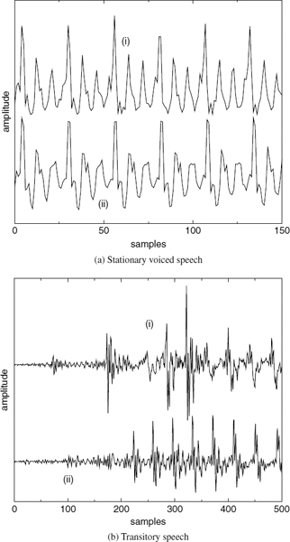
Figure 9.1 Harmonically-synthesized speech

CELP-type coders, such as ACELP [5, 6], encode the target speech waveform directly and perform relatively better at the transitions. However, at low bit-rates, analysis-by-synthesis (AbS) coders fail to synthesize stationary segments with adequate quality. As the bit rate is reduced, they cannot maintain clear periodicity of the stationary voiced segments [7]. CELP-type AbS coders perform waveform-matching for each frame or subframe and select the best possible excitation vector. This process does not consider the pitch cycles of the target waveform, and consecutive synthesized pitch cycles show subtle differences in the waveform shape. This artifact introduces granular noise into the voiced speech, perceptible up to about 6 kb/s. Preserving the periodicity of voiced speech is essential for high quality speech reproduction. Figure 9.2a shows a stationary voiced segment and 9.2b shows a transitory segment synthesized using ACELP at 4kb/s. In Figure 9.2a, the consecutive pitch cycles have different shapes, which degrades the slowly-evolving periodicity of voiced speech, compared to Figure 9.1a. Therefore despite the fact that waveform similarity is less in Figure 9.1a, harmonically-synthesized voiced speech is perceptually superior to waveform-coded speech at low bit-rates. Figure 9.2b shows that ACELP can synthesize the highly nonstationary speech transitions better than harmonic coders (see Figure 9.1b). ACELP may also introduce granular noise at the transitions. However, the speech waveform changes rapidly at the transitions, masking the granular noise of ACELP, which is not perceptible down to about 4kb/s. The above observations suggest a hybrid coding approach, which selects the optimum coding algorithm for a given segment of speech: coding stationary voiced segments using harmonic coding and transitions using ACELP. Unvoiced and silence segments can be encoded with CELP [8] or white-noise excitation.

Harmonic coders suffer from other potential problems such as voicing and pitch errors that may occur at the transitions. The pitch estimates at the transitions, especially at the onsets may be unreliable due to the rapidly-changing speech waveform. Furthermore, pitch-tracking algorithms do not have history at the onsets and should be turned off. Inaccurate pitch estimates also account for inaccurate voicing decisions, in addition to the spectral mismatches due to the nonstationary speech waveform at the transitions. These voicing decision errors declare the voiced bands as unvoiced and increase the hoarseness of synthetic speech. Encoding the transitions using ACELP eliminates those potential problems of harmonic coding.

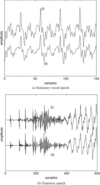
Figure 9.2 Speech synthesized using ACELP

9.2 Design Challenges of a Hybrid Coder

The main challenges in designing a hybrid coder are reliable speech classification and phase synchronization when switching between the coding modes. Furthermore, most of the speech-coding techniques make use of a look-ahead and parameter interpolation. Interpolation requires the parameters of the previous frame; when switched from a different mode, those parameters may not be directly available. Predictive quantization schemes also require the previous memory. Techniques which eliminate these initialization/memory problems are required.

9.2.1 Reliable Speech Classification

A voice activity detector (VAD) can be used to identify speech and silence segments [9], while classification of speech into voiced and unvoiced segments can be seen as the most basic speech classification technique. However, there are coders in the literature which use up to six phonetic classes [10]. The design of such a phonetic classification algorithm can be complicated and computationally complex, and a simple classification with two or three modes is sufficient to exploit the relative merits of waveform and harmonic coding methods. The accuracy of the speech classification is critical for the performance of a hybrid coder. For example, using noise excitation for a stationary voiced segment (which should operate in harmonic coding mode) can severely degrade the speech quality, by converting the high-voiced energy of the original speech into noise in the synthesized speech; use of harmonic excitation for unvoiced segments gives a tonal artifact. ACELP can generally maintain acceptable quality for all the types of speech since it has waveform-matching capability. During the speech classification process, it is essential that the above cases are taken into account to generate a fail-safe mode selection.

9.2.2 Phase Synchronization

Harmonic coders operating at 4 kb/s and below do not transmit phase information, in order to allocate the available bits for accurate quantization of the more important spectral magnitude information. They exploit the fact that the human ear is partially phase-insensitive and the waveform shape of the synthesized speech can be very different from the original speech, often yielding negative SNRs. On the other hand, AbS coders preserve the waveform similarity. Direct switching between those two modes without any precautions will severely degrade the speech quality due to phase discontinuities.

9.3 Summary of Hybrid Coders

The hybrid coding concept has been introduced in the LPC vocoder [11], which classifies speech frames into voiced or unvoiced, and synthesizes the excitation using periodic pulses or white noise, respectively. Analysis-by-synthesis CELP coders with dynamic bit allocation (DBA), which adaptively distribute the bits among coder parameters in a given frame while maintaining a constant bit rate, by classifying each frame into a certain mode, have also been reported [12]. However, we particularly focus here on hybrid coders, which combine AbS coding and harmonic coding. The advantages and disadvantages of harmonic coding and CELP, and the potential benefits of combining the two methods have been discussed by Trancoso et al. [13]. Improving the speech quality of the LPC vocoder by using a form of multi-pulse excitation [14] as a third excitation model at the transitions has also been reported [15].

9.3.1 Prototype Waveform Interpolation Coder

Kleijn introduced prototype waveform interpolation (PWI) in order to improve the quality of voiced speech [7]. The PWI technique extracts prototype pitch cycle waveforms from the voiced speech at regular intervals of 20–30 ms. Speech is reconstructed by interpolating the pitch cycles between the update points. The PWI technique can be applied either directly to the speech signal or to the LPC residual. Since the PWI technique is not suitable for encoding unvoiced speech segments, unvoiced speech is synthesized using CELP. Even though the motivation behind using two coding techniques is different in the PWI coder (i.e. waveform coding is not used for transitions), it combines harmonic coding and AbS coding. The speech classification of the PWI coder is relatively easier, since it only needs to classify speech into either voiced or unvoiced.

At the onset of a voiced section, the previously estimated prototype wave-form is not present at the decoder for the interpolation process. Kleijn suggests three methods to solve this problem:

• Extract the prototype waveform from the reconstructed CELP waveform of the previous frame.
• Set to a single pulse waveform (filtered through LPC) with its amplitude determined from the transmitted information.
• Use a replica of the prototype transmitted at the end of the current synthesis frame.

The starting phase of the pitch cycles at the onsets can be determined at the decoder from the CELP encoded signal. At the offsets, the linear phase deviation between the harmonically synthesized and original speech is measured and the original speech buffer is displaced, such that the AbS coder begins exactly where the harmonic coder ended.

9.3.2 Combined Harmonic and Waveform Coding at Low Bit-Rates

This coder, proposed by Shlomot et al., consists of three modes: harmonic, transition, and unvoiced [16, 17]. All the modes are based on the source filter model. The harmonic mode consists of two components: the lower part of the spectrum or the harmonic bandwidth, which is synthesized as a sum of coherent sinusoids, and the upper part of the spectrum, which is synthesized using sinusoids of random phases. The transitions are synthesized using pulse excitation, similar to ACELP, and the unvoiced segments are synthesized using white-noise excitation.

Speech classification is performed by a neural network, which takes into account the speech parameters of the previous, current, and future frames, and the previous mode decision. The classification parameters include the speech energy, spectral tilt, zero-crossing rate, residual peakiness, residual harmonic matching SNRs, and pitch deviation measures. At the onsets, when switching from the waveform-coding mode, the harmonic excitation is synchronized by shifting and maximizing the cross-correlation with the waveform-coded excitation. At the offsets, the waveform-coding target is shifted to maximize the cross-correlation with the harmonically-synthesized speech, similar to the PWI coder.

9.3.3 A 4 kb/s Hybrid MELP/CELP Coder

The 4 kb/s hybrid MELP/CELP coder with alignment phase encoding and zero phase equalization proposed by Stachurski et al. consists of three modes: strongly-voiced, weakly-voiced, and unvoiced [18, 19]. The weakly-voiced mode includes transitions and plosives, which is used when neither strongly-voiced nor unvoiced speech segments are clearly identified. In the strongly-voiced mode, a mixed excitation linear prediction (MELP) [20, 21] coder is used. Weakly-voiced and unvoiced modes are synthesized using CELP. In unvoiced frames, the LPC excitation is generated from a fixed stochastic codebook. In weakly-voiced frames, the LPC excitation consists of the sum of a long-term prediction filter output and a fixed innovation sequence containing a limited number of pulses, similar to ACELP.

The speech classification is based on the estimated voicing strength and pitch. The signal continuity at the mode transitions is preserved by transmitting an ‘alignment phase’ for MELP-encoded frames, and by using ‘zero phase equalization’ for transitional frames. The alignment phase preserves the time-synchrony between the original and synthesized speech. The alignment phase is estimated as the linear phase required in the MELP-encoded excitation generation to maximize the cross-correlation between the MELP excitation and the corresponding LPC residual. Zero-phase equalization modifies the CELP target signal, in order to reduce the phase discontinuities, by removing the phase component, which is not coded in MELP. Zero phase equalization is implemented in the LPC residual domain, with a Finite Impulse Response (FIR) filter similar to [22]. The FIR filter coefficients are derived from the smoothed pitch pulse waveforms of the LPC residual signal. For unvoiced frames the filter coefficients are set to an impulse so that the filtering has no effect. The AbS target is generated by filtering the zero-phase-equalized residual signal through the LPC synthesis filter.

9.3.4 Limitations of Existing Hybrid Coders

PWI coders and low bit-rate coders that combine harmonic and waveform coding use similar techniques to ensure signal continuity. At the onsets, the initial phases of the harmonic excitation are extracted from the previous excitation vector of the waveform-coding mode. This can be difficult at rapidly-varying onsets, especially if the bit-rate of the waveform coder is low. Moreover, inaccuracies in the onset synchronization will propagate through the harmonic excitation and make the offset synchronization more difficult. At the offsets, the linear phase deviation between the harmonically-synthesized and original speech is measured and the original speech buffer is displaced, such that the AbS coder begins exactly where the harmonic coder has ended. This method needs the accumulated displacement to be reset during unvoiced or silent segments, and may fail to meet the specifications of a system with strict delay requirements.

Another problem arises when a transition occurs within a voiced speech segment as shown in Figure 9.3, where there are no unvoiced or silent segments after the transition to reset the accumulated displacement. Even though the accumulated displacement can be minimized by inserting or eliminating exactly complete pitch cycles, the remainder will propagate into the next harmonic section. Furthermore, a displacement of a fraction of a sample can introduce audible high frequency distortion, especially in segments with short pitch periods. Consequently, the displacements should be performed with a high resolution. The MELP/CELP coder preserves signal continuity by transmitting an alignment phase for MELP-encoded frames and using zero phase equalization for transitional frames. Zero phase equalization may reduce the benefits of AbS coding by modifying the phase spectrum, and it has been reported that the phase spectrum is perceptually important [23–25]. Furthermore, zero phase equalization relies on accurate pitch pulse position detection at the transitions, which can be difficult.

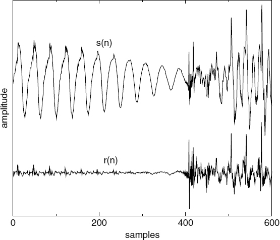
Figure 9.3 A transition within voiced speech

Harmonic excitation can be synchronized with the LPC residual by transmitting the phases, which eliminates the above difficulties. However this requires a prohibitive capacity making it unsuitable for low bit-rate applications. As a compromise, Katugampala [26] proposed a new phase model for the harmonic excitation called synchronized waveform-matched phase model (SWPM). SWPM facilitates the integration of harmonic and AbS coders, by synchronizing the harmonic excitation with the LPC residual. SWPM requires only two parameters and does not alter the perceptual quality of the harmonically-synthesized speech. It also allows the ACELP mode to target the speech waveform without modifying the perceptually-important phase components or the frame boundaries.

9.4 Synchronized Waveform-Matched Phase Model

The SWPM maintains the time-synchrony between the original and the harmonically-synthesized speech by transmitting the pitch pulse location (PPL) closest to each synthesis frame boundary [27, 28, 26]. The SWPM also preserves sufficient waveform similarity, such that switching between the coding modes is transparent, by transmitting a phase value that indicates the pitch pulse shape (PPS) of the corresponding pitch pulse. PPL and PPS are estimated in every frame of 20 ms. SWPM needs to detect the pitch pulses only in the stationary voiced segments, which is somewhat easier than detecting the pitch pulses in the transitions as in [18]. The SWPM has the disadvantage of transmitting two extra parameters (PPL and PPS) but the bottleneck of the bit allocation of hybrid coders is usually in the waveform-coding mode. Furthermore, in stationary voiced segments the location of the pitch pulses can be predicted with high accuracy, and only an error needs to be transmitted. The same argument applies to the shape of the pitch pulses.

In the harmonic synthesis, cubic phase interpolation [2] is applied between the pitch pulse locations, setting the phases of all the harmonics equal to PPS. This makes the waveform similarity between the original and the synthesized speech highest in the vicinity of the selected pitch pulse locations. However this does not cause difficulties, since switching is restricted to frame boundaries and the pitch pulse locations closest to the frame boundaries are selected. Furthermore, SWPM can synchronize the synthesized excitation and the LPC residual with fractional sample resolutions, even without up-sampling either of the waveforms.

9.4.1 Extraction of the Pitch Pulse Location

The TIA Enhanced Variable Rate Coder (EVRC) [29], which employs relaxed CELP (RCELP) [30], uses a simple method based on the energy of the LPC residual to detect the pitch pulses. EVRC determines the pitch pulse locations by searching for a maximum in a five-sample sliding energy window within a region larger than the pitch period, and then finding the rest of the pitch pulses by searching recursively at a separation of one pitch period. It is possible to improve the performance of the residual-energy-based pitch pulse location detection by using the Hilbert envelope of windowed LP residual (HEWLPR) [31, 32]. A robust pitch pulse detection algorithm based on the group delay of the phase spectrum has also been reported [33], however this method has a very high computational complexity.

The SWPM requires a pitch pulse detection algorithm that can detect the pulses at stationary voiced segments with a high accuracy and has a low computational complexity. However the ability to detect the pitch pulses at the onsets and offsets is beneficial, since this will increase the flexibility of transition detection. Therefore an improved pitch pulse detection algorithm, based on the algorithm used in EVRC, is developed for SWPM. Figure 9.4 depicts a block diagram of the pitch pulse location detection algorithm. Initially, all the possible pitch pulse locations are determined by considering the localized energy of the LPC residual and an adaptive threshold function, t(n). The localized energy, e(n), of the LPC residual, r(n), is given by,

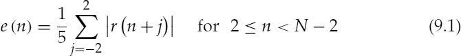
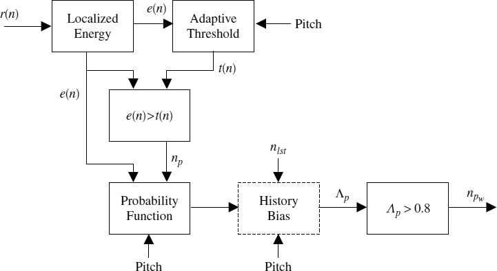
Figure 9.4 Block diagram of the pitch pulse detection algorithm

where N = 240 is the length of the residual buffer.

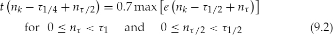
The adaptive threshold function, t(n), is updated for each half pitch period, by taking 0.7 of the maximum of e(n) in the pitch period symmetrically-centred around the half pitch period chosen to calculate t(n), and t(n) is given by,

where , , , n_k = kτ_1/2 for , and τ is the pitch period.

The exceptions corresponding to the analysis frame boundaries are given in,

The sample locations, for which e(n) > t(n), are considered as the regions which may contain pitch pulses. If e(n) > t(n) for more than eight consecutive samples, those regions are ignored, since in those regions the residual energy is smeared, which is not a feature of pitch pulses. The centre of the each remaining region is taken as a possible pitch pulse location, n_p. If any of the two candidate locations are closer than eight samples (i.e. half of the minimum pitch), the one which has the higher e(n_p) is taken.

Applying an adaptive threshold to estimate the pitch pulse locations from the localized energy e(n) is advantageous, especially for segments where the energy of the LPC residual varies rapidly, giving rise to spurious pulses. Figure 9.5 demonstrates this for a male offset and a female onset. The male speech segment has a pitch period of about 80 samples and the two high-energy irregular pulses which do not belong to the pitch contour are clearly visible. The female speech segment has a pitch of about 45 samples, which also contains two high-energy irregular pulses. The energy function e(n) and the threshold function t(n) are also depicted in Figure 9.5, shifted upwards for clarity. The figures also show that e(n) at the irregular pulses may be higher than e(n) at the correct pitch pulses. Therefore selecting the highest e(n) to detect a pitch pulse location as in [34] may lead to errors. Since e(n) > t(n), for some of the irregular pulses as well as for correct pitch pulse locations, further refinements are required. Moreover, the regions where e(n) > t(n), gives only a crude estimation of the pitch pulse location. The algorithm relies on the accuracy of the estimated pitch used for the computation of t(n) and in the refinement process described below. However SWPM needs only the pitch pulses in the stationary voiced segments, for which the pitch estimate is reliable.

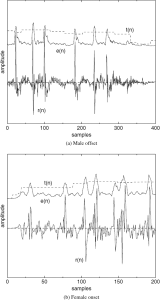
Figure 9.5 Irregular pulses at the onsets and offsets

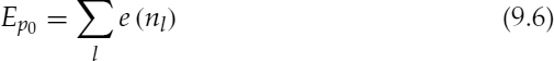
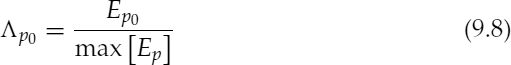
For each selected location n_p, the probability of it being a pitch pulse is estimated, using the pitch and the energy of the neighbouring locations. First, a total energy metric, E_p0 for the candidate pulse at n_p0 is computed recursively as follows,

where l = p₀ and any q which satisfies the condition,

For each term, +τ and −τ, if more than one q satisfies equation (9.7), only the one which minimizes |n_l ± τ − n_q| is chosen. Then further locations n_q that satisfy equation (9.7) are searched recursively, with any n_q which have already satisfied equation (9.7) taken as n_l in the next iteration. Therefore, E_p0 can be defined as the sum of e(n_p) of the pitch contour corresponding to the location n_p0. This process eliminates the high-energy irregular pulses, since they do not form a proper pitch contour and equation (9.7) detects them as isolated pulses. The probability of the candidate location, n_p0, containing a pitch pulse, Λ_p0, is given by,

If pitch pulse locations were detected in the previous frame and any of the current candidate pitch pulse locations form a pitch contour which is a continuation of the previous pitch contour, a history bias term is added. Adding the history bias term enhances the performance at the offsets, especially at the resonating tails. Furthermore, the history bias helps to maintain the continuity of the pitch contour between the frames, at the segments, where the pitch pulses become less significant, as shown in Figure 9.6. A discontinuity in the pitch contour adds a reverberant character into voiced speech segments. The biased term for any location n_l which satisfies equations (9.10) or (9.11) is given by,

The initial value for l is given by equation (9.10), with being the minimum possible integer value which satisfies equation (9.10). If more than one l satisfies equation (9.10) with the same minimum , the one which maximizes e(nl) is taken.

where n_lst is the pitch pulse location selected in the last analysis frame. Then any location n_q which satisfies equation (9.11) is searched and further n_l are found recursively, with any n_q which have already satisfied equation (9.11) taken as n_l in the next iteration. If more than one n_q satisfies equation (9.11), the one which minimizes |n_l + τ + n_q| is chosen.

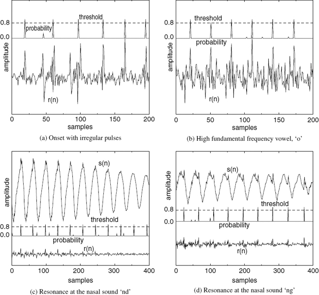
Figure 9.6 Some instances of difficult pitch pulse extraction

The final probability of the candidate location n_p0 containing a pitch pulse Λ_p0 is recalculated,

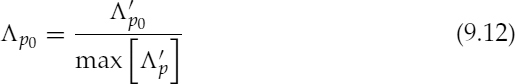
A set of positions, n_pw which have probabilities, Λ_p > 0.8, are selected as the pitch pulse locations, and they are further refined in order to select the pitch pulse closest to the synthesis frame boundary. Figure 9.6 shows some instances of difficult pitch pulse detection along with the estimated probabilities, Λ_p, and the threshold value. In Figures 9.6c and 9.6d, the resonating speech waveforms are also shown.

The problem illustrated in Figure 9.6b can be explained in both the time and frequency domains. In speech segments with a short pitch period, the short-term LPC prediction tends to remove some of the pitch correlation as well, leaving an LPC residual without any clearly distinguishable peaks. Shorter pitch periods in the time domain correspond to fewer harmonics in the frequency domain. Hence the inter-harmonic spacing becomes wider and the formants of the short-term predictor tend to coincide with some of the harmonics (see Figure 9.7). The speech spectrum in Figure 9.7 is lowered by 80 dB in order to emphasize the coinciding points of the spectra. The excessive removal of some of the harmonic components by the LPC filter disperses the energy of the residual pitch pulses. It has been reported that large errors in the linear prediction coefficients occur in the analysis of sounds with high pitch frequencies [35]. In the case of nasal sounds, the speech waveform has a very high low-frequency content (see Figure 9.6c). In such cases, the LPC filter simply places a pole at the fundamental frequency. A pole in the LPC synthesis filter translates to a zero in the inverse filter, giving rise to a fairly random-looking LPC residual signal. The figures demonstrate that the estimated probabilities, Λ_p exceed the threshold value only at the required pitch pulse locations, despite those difficulties.

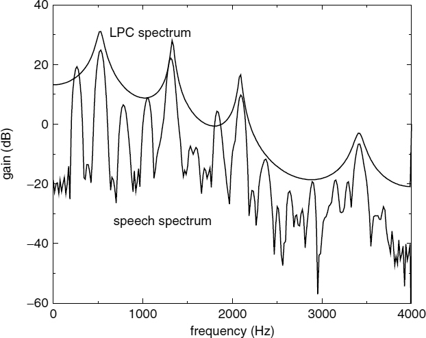
Figure 9.7 Speech and LPC spectra of a female vowel segment

9.4.2 Estimation of the Pitch Pulse Shape

Figure 9.8 depicts a complete pitch cycle of the LPC residual, which includes a selected pitch pulse, and the positive half of the wrapped phase spectrum obtained from its DFT. The integer pitch pulse position is taken as the time origin of the DFT, and the phase spectrum indicates that most of the harmonic phases are close to an average value. This average phase value varies with the shape of the pitch pulse, hence it is called pitch pulse shape (PPS). In the absence of a strong pitch pulse, the phase spectrum becomes random and varies between −π and π.

Figure 9.9 depicts a block diagram of the pitch pulse shape estimation algorithm. This algorithm employs an AbS technique in the time domain to estimate PPS. A prototype pulse, P(n_s), is synthesized as follows:

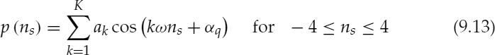
where ω = 2π/τ, τ is the pitch period, K is the number of harmonics, a_k are the harmonic amplitudes, and the candidate pitch pulse shapes, α_q, are given by,

Figure 9.10 depicts the synthesized pulses, p(n_s), for two different candidate pitch pulse shapes, i.e. values of α_q. A simpler solution to avoid estimating the spectral amplitudes, a_k for equation (9.13) is to assume a flat spectrum. However, the use of spectral amplitudes, a_k, gives the relative weight for each harmonic, which is beneficial in estimating the pitch pulse shape. For example, if a harmonic component which is relatively small in the LPC residual signal is given equal weight in the prototype pulse, p(n_s), this may lead to inaccurate estimates in the subsequent AbS refinement process. Considering the frequency domain, those relatively small amplitudes may be affected by spectral leakage from the larger amplitudes, giving large errors in the phase spectrum. However, since computing the spectral amplitudes for each pitch pulse is a very intensive process, as a compromise, the same spectral amplitudes are used for the whole analysis frame, and are also transmitted to the decoder as the harmonic amplitudes of the LPC residual. Then the normalized cross-correlation, R_j, and SNR, E_j, are estimated between the synthesized prototype pitch pulse p(n_s) and each of the detected LPC residual pitch pulses, at the locations n_p, where n_p ∈ n_pw. R_j and E_j are estimated for each candidate pitch pulse shape, α_q,

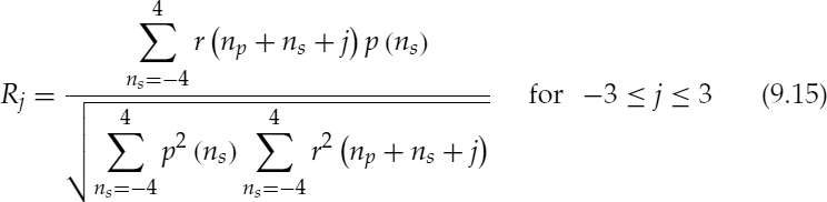
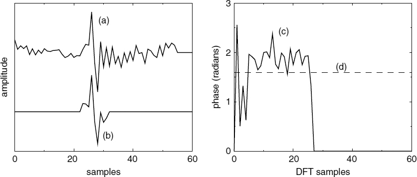
Figure 9.8 (a) a complete pitch cycle of the LPC residual, (b) the pitch pulse synthesized using PPS, (c) the positive half of the phase spectrum obtained from the DFT, and (d) the estimated PPS

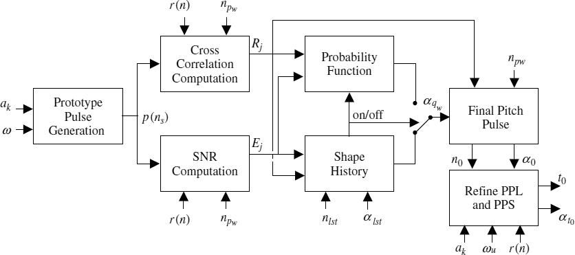
Figure 9.9 Block diagram of the pitch pulse shape estimation

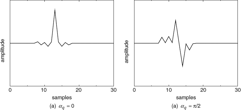
Figure 9.10 synthesized pulses, p(n_s)

The term j is introduced in R_j and E_j in order to shift the relative positioning of the LPC residual pulse and the synthesized pulse. This compensates for the approximate pitch pulse locations, n_p, estimated by the algorithm described in Section 9.4.1, by allowing the initial estimates to shift around, with a resolution of one sample. All the combinations of n_p, α_q, and j for which E_j ≤ 1.0 are excluded from any further processing. E_j ≤ 1.0 corresponds to an SNR of less than or equal to 0 dB. Then probability of the candidate shape, α_q0, being the pitch pulse shape is estimated,

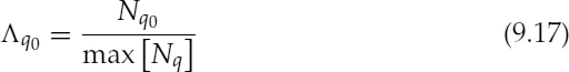
where N_q is the total number of residual pulses for a given q, for which R_j > 0.5. If more than one j satisfies the condition R_j > 0.5, for a particular set of q and n_p, N_q is incremented only once. The set of pitch pulse shape values, α_qw, which have probabilities, Λq > 0.7 are chosen for further refinement. If max [N_q] is zero, then all the Λ_q are set to zero, i.e. no pitch pulses are detected. Figure 9.11 shows the LPC residual of an analysis frame and the estimated probability density function (PDF) of α_q in the range −π ≤ α_q < π. The pitch pulses of the LPC residual in Figure 9.11a have similar shapes to the shape of the synthesized pulse shown in Figure 9.10a. Consequently the PDF is maximum around α_q = 0, for the pitch pulse shape used to synthesize the pulse shown in Figure 9.10a. If a history bias is used in pitch pulse location detection, then the probability term, Λ_q is not estimated. Instead the pitch pulse shape search is limited to three candidates, α_L, around the pitch pulse shape of the previous frame. During the voiced segments, the pitch pulse shape is fairly stationary and restricting the search range around the previous value does not reduce the performance. Restricting the search range has advantages such as reduced computational complexity and efficient differential quantization of the pitch pulse shape. Furthermore, restricting the search range avoids large variations in the pitch pulse shape. Large variations in the pitch pulse shape introduce a reverberant character into the synthesized speech.

Figure 9.11 An analysis frame and the probability density function of α_q,

where,

Then R_j and E_j are estimated as before, substituting α_q with α_L, and all the combinations of n_p, α_L, and j for which E_j ≤ 1.0 or R_j ≤ 0.5 are excluded from any further refinements. If no combination of n_p, α_L, and j are left, the search is extended to all the α_q, and Λ_q is estimated as before, otherwise the remaining α_L are chosen for further refinement, i.e. the remaining α_L form the set α_qw. The pitch pulse closest to the centre of the analysis frame, i.e. closest to the synthesis frame boundary for which R_j > ξ is selected as the final pitch pulse. The threshold value, ξ, is given by,

If more than one set of j and α_q satisfy the condition R_j > ξ for the same pitch pulse closest to the synthesis frame boundary, the set of values which maximizes R_j is chosen. The pitch pulse shape and the integer pitch pulse location are given by the chosen, α_q and n_p + j respectively. Figure 9.11a shows the centre of the analysis frame and the selected pitch pulse. It is also possible to select the pitch pulse closest to the centre of the analysis frame from the set n_pw and estimate the shape of the selected pulse. However estimating the PDF of α_q for the whole analysis frame and including it in the selection process improves the reliability of the estimates, which enables the selection of the most probable α_q. Then the integer pitch pulse location is refined to a 0.125 sample accuracy, and the initial pitch pulse shape is refined to a 2π/64 accuracy. In the refinement process, a synthetic pulse p_u(n_u) is generated in an eight times up-sampled domain, i.e. at 64 kHz. If the selected integer pitch pulse location and shape are n₀ and α₀, respectively, then,

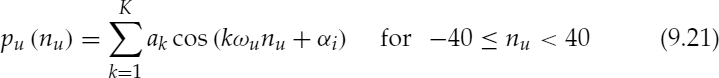
where ω_u = 2π/8τ, and α_i is given by,

Then equation (9.23) is used to compute the normalized cross-correlation R, for all i and j, and the indices corresponding to the maximum R_{i, j} are used to evaluate the refined PPS and PPL, as shown in equations (9.22) and (9.25) respectively.

where p_j(n_r), is the shifted and down-sampled version of p_u(n_u) given by,

The final PPL, t₀, refined to a 0.125 sample resolution is given by,

Fractional PPL is important for segments with short pitch periods and when the pitch pulse is close to or at the synthesis frame boundary. When the pitch period is short, a small variation in the pitch pulse location can induce a large percentage pitch error. The pitch pulses closest to the synthesis frame boundaries are chosen in SWPM in order to maximize the waveform similarity at the frame boundaries, since the mode changes are limited to synthesis frame boundaries. However if the selected pitch pulse is on the frame boundary or within a few samples of it, the pulse must be synthesized smoothly across this boundary, in order to avoid audible artifacts. In such cases, high resolution PPL and PPS are essential to maintain the phase continuity across the frame boundaries. It is also possible to compute the cross-correlation between p_u(n_u) and the eight times up-sampled residual signal, in order to evaluate the best indices i and j. However this requires more computations and an equally good result is obtained by shifting p_u(n_u) in the up-sampled domain and then computing the cross-correlation in the down-sampled domain, as shown in equations (9.23) and (9.24).

At the offsets, if no pitch pulses are detected, PPL is predicted from the PPL of the previous frame using the pitch, and PPS is set to equal to the PPS of the previous frame. This does not introduce any deteriorating artifacts, since the encoder checks the suitability of the harmonic excitation in the mode selection process. The prediction of PPL and PPS is particularly useful at offsets with a resonant tail, where pitch pulse detection is difficult.

9.4.3 Synthesis using Generalized Cubic Phase Interpolation

In the synthesis, the phases are interpolated cubically, i.e. by quadratic interpolation of the frequencies. In [2], phases are interpolated for the frequencies and phases available at the frame boundaries. But in the case of SWPM the frequencies are available at the frame boundaries and the phases at the pitch pulse locations. Therefore a generalized cubic phase interpolation formula is used, to incorporate PPL and PPS.

The phase θ_k(n) of the k^th harmonic of the i + 1^th synthesis frame is given by,

where N is the number of samples per frame and θ_ki and ω_i are the phase of the k^th harmonic and the fundamental frequency, respectively, at the end of synthesis frame i, and α_k and β_k are given by,

where t₀ is the fractional pitch pulse location (PPL), θ_t0 is the PPS estimated at t₀, and M_k represents the phase unwrapping and is chosen according to the ‘maximally smooth’ criterion used by McAulay [2]. McAulay chose M_k such that f (M_k) is a minimum,

where θ_k (t, M_k) represents the continuous analogue form of θ_k(n), and is the second derivative of θ_k (t, M_k) with respect to t. Although M_k is integer-valued, since f (M_k) is quadratic in M_k, the problem is most easily solved by minimizing f (x_k) with respect to the continuous variable x_k and then choosing M_k to be an integer closest to x_k. For the generalized case of SWPM, f (x_k) is minimized with respect to x_k and x_kmin is given by,

is substituted in equation 9.27 for M_k to solve for α_k and β_k and in turn to unwrap the cubic phase interpolation function θ_k(n).

The initial phase θ_ki for the next frame is θ_k(N), and the above computations should be repeated for each harmonic, i.e. k. It should be noted that there is no need to synthesize the phases, θ_k(n) in the up-sampled domain, in order to use the fractional pitch pulse location, t₀. It is sufficient to use t₀ in solving the coefficients of θ_k(n), i.e. α_k and β_k.

9.5 Hybrid Encoder

A simplified block diagram of a typical hybrid encoder that operates on a fixed frame size of 160 samples is shown in Figure 9.12. For each frame, the mode that gives the optimum performance is selected. There are three possible modes: scaled white noise coloured by LPC for unvoiced segments; ACELP for transitions; and harmonic excitation for stationary voiced segments. Any waveform-coding technique can be used instead of ACELP. In fact this hybrid model [27] does not restrict the choice of coding technique for speech transitions, it merely makes the mode decision and defines the target waveform. In white noise excited mode, the gain estimated from the LPC residual energy is transmitted for every 20 ms. The LPC parameters are common for all the modes and estimated every 20 ms (with a 25 ms window length), which are usually interpolated in the LSF domain for every subframe in the synthesis process. In order to interpolate the LSFs, the LPC analysis window is usually centred at the synthesis frame boundary which requires a look-ahead.

Figure 9.12 Block diagram of the hybrid encoder

A two-stage speech classification algorithm is used in the above coder. An initial classification is made based on the tracked energy, low-band to high-band energy ratio, and zero-crossing rate, and determines whether to use the noise excitation or one of the other modes. The secondary classification, which is based on an AbS process, makes a choice between the harmonic excitation or ACELP. Segments of plosives with high-energy spikes are synthesized using ACELP. When the noise excitation mode is selected, there is no need to estimate the excitation parameters of the other modes. If noise excitation is not selected, the harmonic parameters are always estimated and the harmonic excitation is generated at the encoder for the AbS transition detection. The speech classification is described in detail in Section 9.6.

For simplicity, details of LPC and adaptive codebook memory update are excluded from the block diagram. The encoder maintains an LPC synthesis filter synchronized with the decoder, and uses the final memory locations for ACELP and AbS transition detection in the next frame. Adaptive codebook memory is always updated with the previous LPC excitation vector regardless of the mode. In order to maintain the LPC and the adaptive codebook memories, the LPC excitation is generated at the encoder, regardless of the mode.

9.5.1 Synchronized Harmonic Excitation

In the harmonic mode, the pitch and harmonic amplitudes of the LPC residual are estimated for every 20 ms frame. The estimation windows are placed at the end of the synthesis frames, and a look-ahead is used to facilitate the harmonic parameter interpolation. The pitch estimation algorithm is based on the sinusoidal speech-model matching proposed by McAulay [36] and improved by Atkinson [4] and Villette [37, 38]. The initial pitch is refined to 0.2 sample accuracy using synthetic spectral matching proposed by Griffin [3]. The harmonic amplitudes are estimated by simple peak-picking of the magnitude spectrum of the LPC residual.

The harmonic excitation e_h (n) is generated at the encoder for the AbS transition detection and to maintain the LPC and adaptive codebook memories, which is given by,

where K is the number of harmonics. Since two analysis frames are interpolated to produce a synthesis frame, K is taken as the higher number of harmonics out of the two analysis frames and the missing amplitudes of the other analysis frame are set to zero. N is the number of samples in a synthesis frame and θ_k(n) is given in equation (9.26) for continuing harmonic tracks, i.e. each harmonic of an analysis frame is matched with the corresponding harmonic of the next frame. For terminating harmonics, i.e. when the number of harmonics in the next frame is smaller, θ_k(n) is given by,

where θ_ki is the phase of the harmonic k and τ_i is the pitch at the end of synthesis frame i. For emerging harmonics, θ_k(n) is given by,

where t₀ is the PPL, θ_t0 is the corresponding PPS, and τ_i+1 is the pitch, all at the end of synthesis frame i +1. Continuing harmonic amplitudes are linearly interpolated,

where a_ki is the amplitude estimate of the k^th harmonic at the end of synthesis frame i. For terminating harmonic amplitudes a trapezoidal window, unity for 55 samples and linearly decaying for 50 samples, is applied from the beginning of the synthesis frame,

For emerging harmonic amplitudes a trapezoidal window, linearly rising for 50 samples and unity for 55 samples, is applied starting from the 56^th sample of the synthesis frame,

9.5.2 Advantages and Disadvantages of SWPM

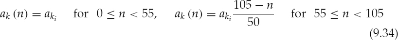
Figure 9.13 shows some examples of waveforms synthesized using the harmonic excitation technique described in Section 9.5.1. In each example, (i) represents the LPC residual or the original speech signal and (ii) represents the LPC excitation or the synthesized speech signal. Figure 9.13a shows the LPC residual and the harmonic excitation of a segment which has strong pitch pulses and Figure 9.13b shows the corresponding speech waveforms. It can be seen that the synthesized speech waveform is very similar to the original. Figure 9.13c shows the LPC residual and the harmonic excitation of a segment which has weak or dispersed pitch pulses and Figure 9.13d shows the corresponding speech waveforms. The synthesized speech is time-synchronized with the original, however the waveform shapes are slightly different, especially between the major pitch pulses. The waveform similarity is highest at the major excitation pulse locations and decreases along the pitch cycles. This is due to the fact that SWPM models only the major pitch pulses and it cannot model the minor pulses present in the residual signal when the LPC residual energy is dispersed. Furthermore, the dispersed energy of the LPC residual, becomes concentrated around the major pitch pulses in the excitation signal. The synthesized speech also exhibits larger variations in the amplitude around the pitch pulse locations, compared with the original speech.

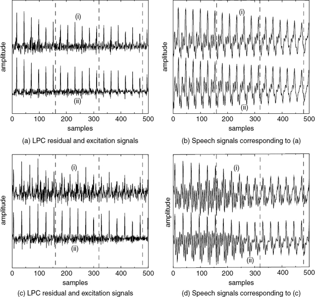
Figure 9.13 synthesized voiced excitation and speech signals

In order to understand the effects on subjective quality due to the above observations, an informal listening test was conducted by switching between the harmonically-synthesized speech and the original speech waveforms at desired synthesis frame boundaries. The informal listening tests showed occasional audible artifacts at the mode transitions, when switching from the harmonic mode to the waveform-coding mode. However there were no audible switching artifacts when switching from waveform-coding to harmonic-coding mode, i.e. at the onsets. It was found that this is due to two reasons: difficulties in reliable pitch pulse detection and limitations in representing the harmonic phases using the pitch pulse shape at some segments. At some highly resonant segments, the LPC residual looks like random noise and it is not possible even to define the pitch pulses. The predicted pitch pulse location, assuming a continuing pitch contour, may be incorrect at resonant tails. At such segments, the pitch pulse locations are determined by applying AbS techniques in the speech domain, such that the synthesized speech signal is synchronized with the original, as described in the next subsection. In the speech segments illustrated using Figure 9.13c, it is possible to detect dominant pitch pulses. However the LPC residual energy is dispersed throughout the pitch periods, making the pitch pulses less significant, as described in Section 9.4.1. This effect reduces the coherence of the LPC residual harmonic phases at the pulse locations and the DFT phase spectrum estimated at the pulse locations look random. Female vowels with short pitch periods show these characteristics. A dispersed phase spectrum reduces the effectiveness of the pitch pulse shape, since the concept of pitch pulse shape is based on the assumption that a pitch pulse is the result of the superimposition of coherent phases, which have the same value at the pitch pulse location. This effect is illustrated in Figure 9.14. The synthesized pitch pulse models the major pulse in the LPC residual pitch period and concentrates the energy at the pulse location. This is due to the single phase value used to synthesize the pulse, as opposed to the more random-looking phase spectrum of the original pitch cycle. This phenomenon introduces phase discontinuities, which accounts for the audible switching artifacts. However the click and pop sounds present at the mode transitions in speech synthesized with SWPM are less annoying than those in a conventional zero-phase excitation, even if the pitch pulse locations are synchronized. This is because SWPM has the additional flexibility of choosing the most suitable phase value (PPS) for pitch pulses, such that the phase discontinuities are minimized. Figure 9.15 illustrates the effect of PPS on the LPC excitation and the synthesized speech signals. For comparison, it includes the original signals and the signals synthesized using the SB-LPC coder [4] which assumes a zero-phase excitation.

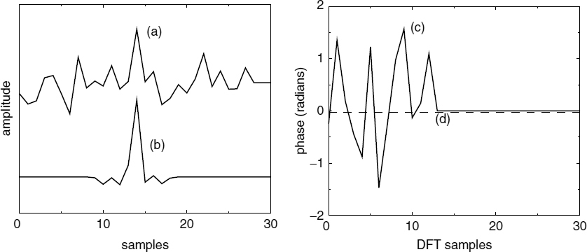
Figure 9.14 PPS at a dispersed pitch period: (a) a complete pitch cycle of the LPC residual, (b) the pitch pulse synthesized using PPS, (c) the positive half of the phase spectrum obtained from the DFT, and (d) estimated PPS

Figure 9.15 Speech synthesized using PPS

The absence of audible switching artifacts at the onsets is an interesting issue. There are two basic reasons for the differences between switching artifacts at the onsets and at the offsets: the nature of the excitation signal and the LPC memory. At the onsets, even though the pitch pulses may be irregular due to the unsettled pitch of the vocal cords, they are quite strong and the residual energy is concentrated around them. Resonating segments and dispersed pulses do not occur at the onsets. Therefore the only difficulty at the onsets is in identifying the correct pulses and, as long as the pulse identification process is successful, SWPM can maintain the continuity of the harmonic phases at the onsets. The pitch pulse detection algorithm described is capable of accurate detection of the pitch pulses at the onsets as described in Section 9.4.1. Furthermore at the onsets, waveform coding preserves the waveform similarity, which also ensures the correct LPC memory, since LPC memory contains the past synthesized speech samples. Therefore the mode transition at the onsets is relatively easier and SWPM guarantees a smooth mode transition at the onsets. However at the offsets, the presence of weak pitch pulses is a common feature and the highly resonant impulse response LPC filter carries on the phase changes caused by the past excitation signal, especially when the LPC filter gain is high. Therefore, the audible switching artifacts remain at some of the offset mode transitions. These need to be treated as special cases.

At the resonant tails the LPC residual looks like random noise, and the pitch pulses are not clearly identifiable. In those cases AbS techniques can be applied directly on the speech signal to synchronize the synthesized speech. This process is applied only for the frames, which follow a harmonic frame and have been classified as transitions.

Synthesized speech is generated by shifting the pitch pulse location (PPL) at the end of the synthesis frame, ±τ/2 around the synthesis frame boundary with a resolution of one sample, where τ is the pitch period. The location which gives the best cross-correlation between the synthesized speech and the original speech is selected as the refined PPL. The pitch pulse shape is set equal to the pitch pulse shape of the previous frame. The excitation and the synthesized speech corresponding to the refined PPL are input to the closed-loop transition detection algorithm, and form the harmonic signal if the transition detection algorithm classifies the corresponding frame as harmonic, otherwise waveform coding is used.

9.5.3 Offset Target Modification

The SWPM minimizes the phase discontinuities at the mode transitions, as described in Section 9.5.2. However at some mode transitions such as the offsets after female vowels, which have dispersed pulses, audible phase discontinuities still remain. These discontinuities may be eliminated by transmitting more phase information. This section describes a more economical solution to remove those remaining phase discontinuities at the offsets, which does not need the transmission of additional information. The proposed method modifies some of the harmonic phases of the first frame of the waveform-coding target, which follows the harmonic mode. The remaining phase discontinuities can be corrected within the first waveform-coding frame, since SWPM keeps the phase discontinuities at a minimum and the pitch periods are synchronized.

As a first approach the harmonic excitation is extended into the next frame and the synthesized speech is linearly interpolated with the original speech at the beginning of the frame in order to produce the waveform-coding target. Listening tests were carried out with different interpolation lengths. The waveform-coding target was not quantized, in order to isolate the distortions due to switching. The tests were extended in order to understand the audibility of the phase discontinuities with the frequency of the harmonics, by manually shifting one phase at a time and synthesizing the rest of the harmonics using the original phases. Phase shifts of π/2 and π are used. Listening tests show that for various interpolation lengths the phase discontinuities below 1 kHz are audible, and an interpolation length as small as 10 samples is sufficient to mask distortions in the higher frequencies. Furthermore, male speech segments with long pitch periods, around 80 samples and above, do not cause audible switching artifacts. Male speech segments with long pitch periods have well-resolved short-term and long-term correlations, and produce clear and sharp pitch pulses, which can be easily modeled by SWPM. Therefore only the harmonics below 1 kHz of the segments with pitch periods shorter than 80 samples are considered in the offset target modification process.

The harmonic excitation is extended beyond the mode transition frame boundary, and the synthesized speech is generated in order to estimate the harmonic phases at the mode transition frame boundary. The phase of the k^th harmonic of the excitation is computed as follows:

where θ_ki is the phase of the k^th harmonic and τ_i is the pitch at the end of synthesis frame i. The excitation signal is given by,

where K is the number of harmonics and a_ki is the amplitude of the k^th harmonic estimated at the end of the synthesis frame i. The excitation signal is filtered through the LPC synthesis filter to produce the synthesized speech signal, with the coefficients estimated at the end of the synthesis frame i. The LPC memories after synthesizing the i^th frame are used as the initial memories. The speech samples synthesized for the i^th and i + 1^th frames are concatenated and windowed with a Kaiser window of 200 samples (β = 6.0) centred at the frame boundary. The harmonic phases, φ_ki, are estimated using a 512 point FFT.

Having analysed the synthesized speech, the original speech is windowed at three points: at the end of the synthesis frame i, at the centre of the synthesis frame i +1, and at the end of the synthesis frame i +1, using the same window function as before. The corresponding harmonic amplitudes, A_ki, A_ki+1/2, A_ki+1 and the phases _ki, _ki+1/2, _ki+1 are estimated using 512 point FFTs. Then the signal component s_l(n), which consists of the harmonics below 1 kHz, is synthesized by,

where L is the number of harmonics below 1 kHz at the end of the i^th synthesis frame, A_k (n) is obtained by linear interpolation between A_ki, A_ki+1/2, and A_ki+1, and Θ_k(n) is obtained by cubic phase interpolation [2] between _ki, _ki+1/2, and _ki+1. Then the signal s_m (n), which has modified phases is synthesized.

and, finally, the modified waveform-coding target of the i + 1^th synthesis frame is computed by,

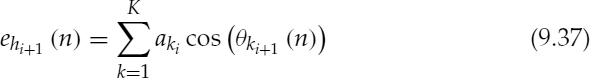
where Φ_k(n) is obtained by cubic phase interpolation between φ_ki and _ki+1 Thus the modified signal, s_m (n) has the phases of the harmonically-synthesized speech at the beginning of the frame and the phases of the original speech at the end of the frame. In other words, (the rate of change of each harmonic phase) is modified such that the phase discontinuities are eliminated, by keeping equal to the harmonic frequencies at the frame boundaries. There is a possibility that such phase modification operations induce a reverberant character in the synthesized signals. However, large phase mismatches close to π are rare, because SWPM minimizes the phase discontinuities. Furthermore, the modifications are applied only for the speech segments, which have pitch periods shorter than 80 samples, thus a phase mismatch is smoothed out in a few pitch cycles. The listening tests confirm that the synthesized speech does not possess a reverberant character. Limiting the phase modification process for the segments with pitch periods shorter than 80 samples also improves the accuracy of the spectral estimations, which use a window length of 200 samples. Figure 9.16 illustrates the waveforms of equation (9.40). It can be seen that the phases of the low frequency components of the original speech waveform, s(n), are modified in order to obtain s_t(n). The waveforms in Figures 9.16c and 9.16d depict s_l(n) and s_m(n), respectively, the low frequency components, which have been modified. The phase relationships between the high-frequency components account more for the perceptual quality of speech [25], and the high-frequency phase components are unchanged in the process.

Figure 9.16 Offset target modification: (a) s(n), (b) s_t(n), (c) s_l(n), and (d) s_m(n)

Some speech signals show rapid variations in the harmonic structure at the offsets, which may reduce the efficiency of the phase modification process. In order to limit those effects the spectral amplitude and phase estimation process is not strictly confined to the harmonics of the fundamental frequency. Instead the amplitude and phase corresponding to the spectral peak closest to each harmonic frequency are estimated. The frequency of the selected spectral peak is taken as the frequency of the estimated amplitude and phase. When finding the spectral peaks closest to the harmonic frequencies, the harmonic frequencies are determined by the fundamental frequency at the end of the i^th synthesis frame, since the pitch estimates at the transition frame are less reliable. In fact the purpose of the offset target modification process is to find the frequency components corresponding to the harmonics of the harmonically-synthesized frame in the i^th frame and change the phase evolution of those components such that the discontinuities are eliminated. Moreover, the same set of spectral peak frequencies and amplitudes are used when synthesizing the terms s_l(n) and s_m(n), hence there is no need to restrict the synthesis process to the pitch harmonics.

Another important issue at the offsets is the energy contour of the synthesized speech. The harmonic coder does not directly control the energy of the synthesized speech, since it transmits the residual energy. However the waveform coders directly control the energy of the synthesized speech, by estimating the excitation gain using the synthesized speech waveform. This may cause discontinuities at the offset mode transition frame boundaries, especially when the LPC filter gain is high. The final target for the waveform coder is produced by linear interpolation between the extended harmonically synthesized speech and the modified target, s_t(n) at the beginning of the frame for 10 samples. The linear interpolation ensures that the discontinuities due to variations of the energy contour are eliminated as well as the phase discontinuities, which are not accounted for in the phase modification process described above.

9.5.4 Onset Harmonic Memory Initialization

The harmonic phase evolution described in Section 9.4.3 and the harmonic excitation described in section 9.5.1 interpolate the harmonic parameters in the synthesis process, and assume that the model parameters are available at the synthesis frame boundaries. However, at the onset mode transitions, when switching from the waveform-coding mode, the harmonic model parameters are not directly available. The initial phases θ_ki, the fundamental frequency ω_i in the phase evolution equation (9.26), and the initial harmonic amplitudes a_ki in equation (9.33) are not available at the onsets. Therefore, they should be estimated at the decoder from the available information. The signal reconstructed by the waveform coder prior to the frame boundary and the harmonic parameters estimated at the end of the synthesis frame boundary are available at the decoder. The use of a waveform-coded signal in estimating the harmonic parameters at the onsets may be unreliable due to two reasons: the speech signal shows large variations at the onsets and, at low bit-rates, the ACELP excitation at the onsets reduces to a few dominant pulses, lowering the reliability of spectral estimates. Therefore the use of waveform-coded signal in estimating the harmonic parameters should be minimized. The waveform-coded signal is used only in initializing the amplitude quantization memories.

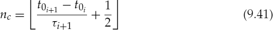
Since preserving the waveform similarity at the frame boundaries is important, the pitch is recomputed such that the previous pitch pulse location can be estimated at the decoder. Therefore the transmitted pitch represents the average over the synthesis frame. The other transmitted harmonic model parameters are unchanged, and are estimated at the end of the synthesis frame boundary. Let's define the pitch, τ_i+1 and pitch pulse location, t_0i+1, at the end of the i + 1^th synthesis frame, and the pitch pulse location at the end of the i^th synthesis frame, t_0i. The number of pitch cycles n_c between t_0i and t_0i+1 is given by,

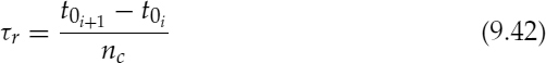
The recomputed pitch, τ_r, is given by,

Then τ_r and t_0i+1 are transmitted, and t_0i is computed at the decoder, as follows,

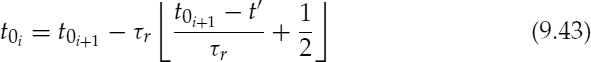
where t′ is the starting frame boundary and t_0i is the pitch pulse location closest to t′. The pitch pulse shape, θ_0i, at the end of the i^th synthesis frame is set equal to the pitch pulse shape, θ_0i+1, at the end of the i + 1^th synthesis frame. The initial phases θ_ki in equation (9.26) are estimated as follows,

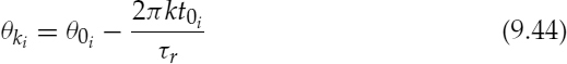
Both fundamental frequency terms, ω_i and ω_i+1, in equation (9.27) are computed using τ_r, i.e. ω_i = ω_i+1 = 2π/τ_r. The harmonic amplitudes a_ki in equation (9.33) are set equal to a_ki+1. Therefore, the phase evolution of the first harmonic frame of a stationary voiced segment becomes effectively linear and the harmonic amplitudes are kept constant, i.e. not interpolated.

9.5.5 White Noise Excitation

Unvoiced speech has a very complicated waveform structure. ACELP can be used to synthesize unvoiced speech and it essentially matches the waveform shape. However, a large number of excitation pulses are required to synthesize the noise-like unvoiced speech. Reducing the number of ACELP excitation pulses introduces sparse excitation artifacts in noise-like segments [39]. The synthesized speech also shows the sparse nature, and the pulse locations are clearly identifiable even in the LPC-synthesized speech. In fact, during unvoiced speech the short term correlation is small and the LPC filter gain has little effect.

Sinusoidal excitation can also be used to synthesize unvoiced segments, despite the fact that there is no harmonic structure. Speech synthesized by generating the magnitude spectrum every 80 samples (100 Hz) and uniformly-distributed random phases for unvoiced segments can achieve good quality [40]. This method suits sinusoidal coders using frequency domain voicing without an explicit time-domain mode decision, since it facilitates the use of the same general analysis and synthesis structure for both voiced and unvoiced speech. However, this hybrid model classifies the unvoiced and silence segments as a separate mode, and, hence, uses a simpler unvoiced excitation generation model, which does not require any frequency-domain transforms. It has been shown that scaled white noise coloured by LPC can produce unvoiced speech with quality equivalent to μ-law logarithmic PCM [41, 42], implying that the complicated waveform structure of unvoiced speech has no perceptual importance. Therefore in terms of the perceptual quality, the phase information transmitted by ACELP is redundant and higher synthesis quality can be achieved at lower bit-rates using scaled white-noise excitation. Figure 9.17 shows a block diagram of the unvoiced gain estimation process and Figure 9.18 shows a block diagram of the unvoiced synthesis process. The band pass filters used are identical and have cut-off frequencies of 140 Hz and 3800 Hz. The transfer function of the fourth-order infinite impulse response (IIR) band pass filters is given by,

and the unvoiced gain, g_uv, is given by,

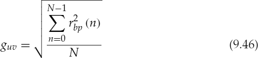
where r_bp(n) is the band-pass-filtered LPC residual signal and N is the length of the residual vector, which is 160 samples including a look-ahead of 80 samples to facilitate overlap and add synthesis at the decoder.

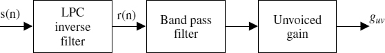
Figure 9.17 Unvoiced gain estimation

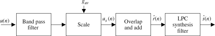
Figure 9.18 Unvoiced synthesis

White noise, u(n), is generated by a random number generator with a Gaussian distribution (a Gaussian noise source has been found to be subjectively superior to a simple uniform noise source). The scaled white-noise excitation, u_s(n), is obtained by,

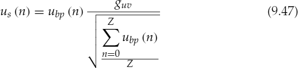
where u_bp(n) is the band-pass-filtered white noise and Z is the length of the noise vector, 240 samples. For overlap and add, a trapezoidal window is used with an overlap of 80 samples. For each synthesis frame the filtered noise buffer, u_bp, is shifted by 80 samples and a new 160 samples are appended, this eliminates the need for energy compensation functions to remove the windowing effects [43]. In fact the overlapped segments are correlated, and the trapezoidal windows do not distort the rms energy.

No attempt is made to preserve the phase continuity when switching to or from the noise excitation. When switching from a different mode, the unvoiced gain, g_uv, of the previous frame is set equal to the current value. The validity of these assumptions are tested through listening tests and the results confirm that these assumptions are reasonable and do not introduce any audible artifacts. The average bit rate can be further reduced by the introduction of voice activity detection (VAD) and comfort noise generation at the decoder for silence segments [9, 44].

9.6 Speech Classification

The speech classification or mode selection techniques can be divided into three categories [45].

• Open-loop mode selection: Each frame is classified based on the observations of parameters extracted from the input speech frame without assessing how the selected mode will perform during synthesis for the frame concerned.
• Closed-loop mode selection: Each frame is synthesized using all the modes and the mode that gives the best performance is selected.
• Hybrid mode selection: The mode selection procedure combines both open-loop and closed-loop approaches. Typically, a subset of modes is first selected by an open-loop procedure, followed by further refinements using closed-loop techniques.

Closed-loop mode selection has two major difficulties: high complexity and difficulty in finding an objective measure which reflects the subjective quality of synthesized speech [46]. The existing closed-loop mode selection coders are based on CELP, and select the best configuration such that the weighted MSE is minimized [47, 48]. Open-loop mode selection is based on techniques such as: voice activity detection, voicing decision, spectral envelope variation, speech energy, and phonetic classification [10]. See [49] for a detailed description on acoustic phonetics.

In the following discussion, a hybrid mode selection technique is used, with an open-loop initial classification and a closed-loop secondary classification. The open loop initial classification decides to use either the noise excitation or one of the other modes. The secondary classification synthesizes the harmonic excitation and makes a closed loop decision to use either the harmonic excitation or ACELP. A special feature of this classifier is the application of closed-loop mode selection to harmonic coding. The SWPM [26] preserves the waveform similarity of the harmonically-synthesized speech, making it possible to apply closed-loop techniques in harmonic coding.

9.6.1 Open-Loop Initial Classification

The initial classification extracts the fully unvoiced and silence segments of speech, which are synthesized using white-noise excitation. It is based on tracked energy, the low-band to high-band energy ratio, and the zero-crossing rate of the speech signal. The three voicing metrics are logically combined to enhance the reliability, since a single metric alone is not sufficient to make a decision with high confidence. The metric combinations and thresholds are determined empirically, by plotting the metrics with the corresponding speech waveforms. A statistical approach is not suitable for deciding the thresholds, because the design of the classification algorithm should consider that a misclassification of a voiced segment as unvoiced will severely degrade the speech quality, but a misclassification of an unvoiced segment as voiced can be tolerated. A misclassified unvoiced segment will be synthesized using ACELP, however a misclassified voiced segment will be synthesized using noise excitation.

The tracked energy of speech, t_e is estimated as follows:

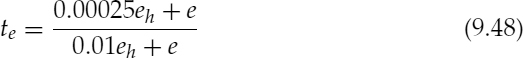
where e is the mean squared speech energy, given by,

where N, the length of the analysis frames, is 160 and e_h is an autoregressive energy term given by,

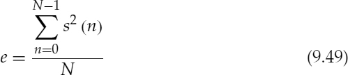
The condition 8e > e_h ensures that e_h is updated only when the speech energy is sufficiently high and e_h should be initialized to approximately the mean squared energy of voiced speech. Figure 9.19a illustrates the tracked energy over a segment of speech. The low-band to high-band energy ratio, γ_ω, is estimated as follows:

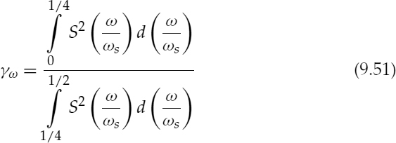
where ω_s is the sampling frequency and S(ω) is the speech spectrum. The speech spectrum is estimated using a 512-point FFT, after windowing 240 speech samples with a Kaiser window of β = 6.0. Figure 9.19b illustrates the low-band to high-band energy ratio over a segment of speech, where the speech signal is shifted down for clarity.

The zero-crossing rate is defined as the number of times the signal changes sign, divided by the number of samples used in the observation. Figure 9.20a illustrates the zero-crossing rate over a segment of speech, where the speech signal is shifted down for clarity. Figure 9.20b depicts the voicing decision made by the initial classification. Figure 9.21 depicts the three metrics used and the final voicing decision over the same speech segment.

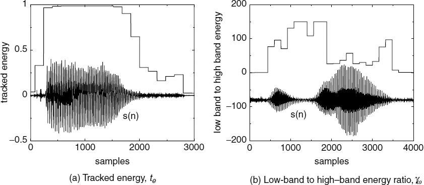
Figure 9.19 Voicing metrics of the initial classification

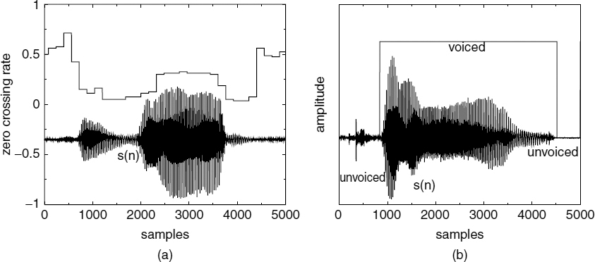
Figure 9.20 (a) Zero-crossing rate and (b) Voicing decision of the initial classification

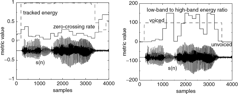
Figure 9.21 Voicing metrics of the initial classification

Even though the plosives have a significant amount of energy at high frequencies and a high zero-crossing rate, synthesizing the high energy spikes of the plosives using ACELP instead of noise excitation improves speech quality. Therefore we need to detect the plosives, which are classified as unvoiced by the initial classification, and switch them to ACELP mode. A typical plosive is depicted at the beginning of the speech segment in Figure 9.20b.

9.6.2 Closed-Loop Transition Detection

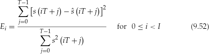
AbS transition detection is performed on the speech segments [26, 27] that are declared voiced by the open-loop initial classification. A block diagram of the AbS classification process is shown in Figure 9.22. The AbS classification module synthesizes speech using SWPM and checks the suitability of the harmonic model for a given frame. The normalized cross-correlation and squared error are computed in both the speech domain and the residual domain for each of the selected pitch cycles within a synthesis frame. The pitch cycles are selected such that they cover the complete synthesis frame. The mode decision between harmonic and ACELP modes is then based on the estimated cross-correlation and squared error values. The squared error of the i^th pitch cycle, E_i, is given by,

The normalized cross-correlation of the i^th pitch cycle, R_i, is given by,

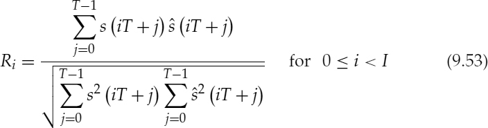
where , τ is the pitch period, , and N is the synthesis frame length of 160 samples.

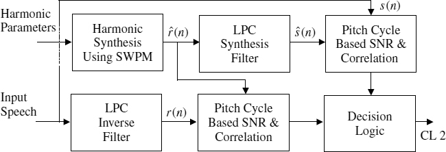
Figure 9.22 Analysis by synthesis classification

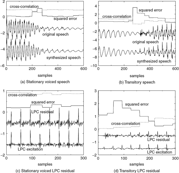
Figure 9.23 Squared error, E_i, E_ir, and cross-correlation, R_i, R_ir, values

In order to estimate the normalized residual cross-correlation, R_ir, and residual squared error, E_ir, equations (9.52) and (9.53) are repeated with s(n) and replaced by r(n) and respectively. Figure 9.23 depicts E_i, R_i, original speech s(n), and synthesized speech . E_i and R_i are aligned with the corresponding pitch cycles of the speech waveforms, and the speech waveforms are shifted down for clarity. Examples of the residual domain signals, LPC residual r(n), LPC excitation , E_ir, and R_ir are also shown in the figure.

For stationary voiced speech, the squared error, E_i, is usually much lower than unity and the normalized cross-correlation, R_i, is close to unity. However, the harmonic model fails at the transitions, which results in larger errors and lower correlation values. The estimated normalized cross-correlation and squared error values are logically combined to increase the reliability of the AbS transition detection. The combinations and thresholds are determined empirically by plotting the parameters with the corresponding speech waveforms. This heuristic approach is superior to a statistical approach, because it allows inclusion of the most important transitions, while the less important ones can be given a lower priority. AbS transition detection compares the harmonically synthesized speech with the original speech, verifies the accuracy of the harmonic model parameters, and decides to use ACELP when the harmonic model fails.

The cross-correlation and squared error values are estimated on the pitch cycle basis in order to determine the suitability of the harmonic excitation for each pitch cycle. Estimating the parameters over the complete synthesis frame may average out a large error caused by a sudden transition. In Figure 9.23a, the speech waveform has a minor transition. The estimated parameters also indicate the presence of such a transition. These minor transitions are synthesized using the harmonic excitation, and the mode is not changed to waveform coding. Changing the mode for these small variations leads to excessive switching, which may degrade the speech quality, when the bit-rate of the waveform coder is relatively low, due to the quantization noise of the waveform coding. Moreover, the harmonic excitation is capable of producing good quality speech despite those small variations in the waveform. In addition to maintaining the harmonic mode across those minor transitions, in order to limit excessive switching, the harmonic mode is not selected after ACELP when the speech energy is rapidly decreasing. Rapidly-decreasing speech energy indicates an offset and at some offsets the coding mode may fluctuate between ACELP and harmonic, if extra restrictions are not imposed. At such offsets, the accumulated error in the LPC memories through the harmonic mode is corrected by switching to the ACELP mode, which in turn causes a switch back to the harmonic mode. The additional measures taken to eliminate those fluctuations are described below.

In order to avoid mode fluctuations at the offsets, extra restrictions are imposed when switching to the harmonic mode after waveform coding. The rms energy of the speech and the LPC residual are computed for each frame, and a hysteresis loop is added using a control flag. The flag is set to zero when the speech or the LPC residual rms energy is less than 0.75 times the corresponding rms energy values of the previous frame. The flag is set to one when the speech or the LPC residual rms energy is more than 1.25 times the corresponding rms energy values of the previous frame. The flag is set to zero if the pitch is greater than 100 samples, regardless of the energy. When switching to harmonic mode after waveform coding, the control flag should be one, in addition to the mode decision of closed-loop transition detection. The flag is checked only at a mode transition, once the harmonic mode is initialized, the flag is ignored. This process avoids excessive switching at the offsets.

The pitch is used to change the control flag for different reasons. For male speech with long pitch periods, ACELP produces better quality than the harmonic coders even at stationary voiced segments. When the pitch period is long, ACELP needs fewer pulses in the time domain to track the changes in the speech waveform while the harmonic coders have to encode a large number of harmonics in the frequency domain. Furthermore, it is well-known that speech-coding schemes which preserve the phase accurately work better for male speech, while the harmonic coders which encode only the amplitude spectrum result in better quality for female speech [24].

9.6.3 Plosive Detection

The unvoiced synthesis process described in Section 9.5.5 updates the unvoiced gain every 20 ms. While this is sufficient for fricatives, it reduces the quality of the highly nonstationary unvoiced components such as plosives. The listening tests show that synthesizing plosives using ACELP preserves the sharpness of the synthesized speech and improves the perceptual quality. Therefore a special case is required to detect the plosives, which are classified as unvoiced by the initial classification, and synthesize them using ACELP.

Plosives are characterized by isolated pulse-like signals with a sharp rise in energy, and this feature is used to distinguish them from the fricatives. The rms energy, e_j, of the speech signal is computed for every 10 samples as follows:

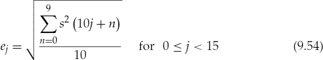
A plosive detection metric, p_j, is defined as,

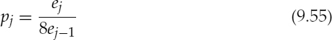
where e₋₁ is the final energy term of the previous frame. A frame is classified as containing a plosive if p_j > 1 for at least one j. This algorithm may signal a plosive even when the overall energy level is very low, for example at a silence segment, if it detects a large fluctuation in energy. Those low-energy segments are completely ignored when using the tracked energy term, t_e, in the open-loop initial classification.

It should be noted that the scope of this plosive detection algorithm is reduced to unvoiced segments, since the segments that include the unvoiced plosives are already identified by the initial classification. The plosive detection algorithm may erroneously identify the highly nonstationary onsets and the speech signal near the glottal excitation of the long pitch period segments as plosives, if applied to voiced speech. Figure 9.24a illustrates the plosive detection metric p_j and an example of a plosive. Figure 9.24b illustrates the detected plosive synthesized using 4 kb/s SB-LPC and 3.7 kb/s ACELP (with-out LTP). ACELP is used only for the frame that has the plosive and the rest of the segment is synthesized using white-noise excitation. SB-LPC synthesizes the speech segment using noise excitation, which cannot adequately represent the plosive.

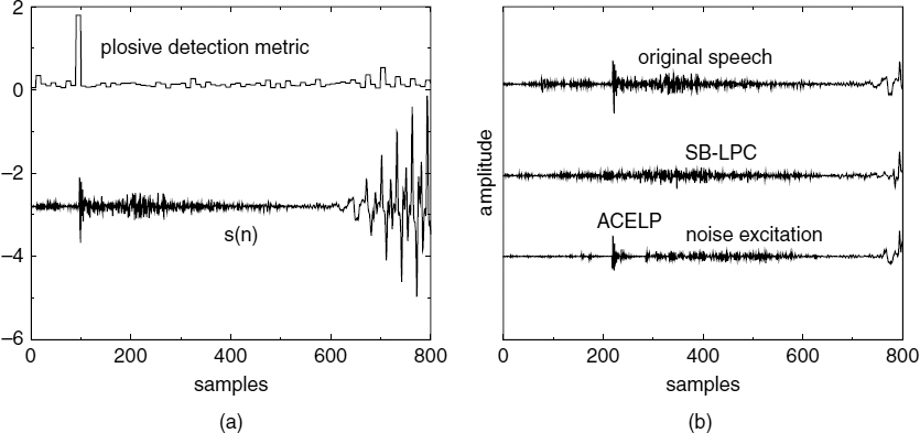
Figure 9.24 Plosive (a) detection and (b) synthesis

9.7 Hybrid Decoder

A simplified block diagram of the hybrid decoder is shown in Figure 9.25. The decoder extracts the excitation parameters from the data bit stream according to the mode and uses the appropriate excitation generation. The synthesized excitation is then fed into the LPC synthesis filter, which produces the final synthetic speech output. The LPC parameters are common for all the modes and linearly interpolated in the LSF domain with an update interval of 5 ms. The excitation vector is also fed into the ACELP excitation and harmonic excitation generators. The ACELP excitation updates the long term prediction (LTP) buffer with the previous LPC excitation. The harmonic excitation uses the previous excitation at the onsets to initialize the interpolation and prediction parameters. In Figure 9.26 the results are shown for the original and synthesized speech together with the mode used for each synthesis frame. The frame boundaries are also shown by dashed lines.

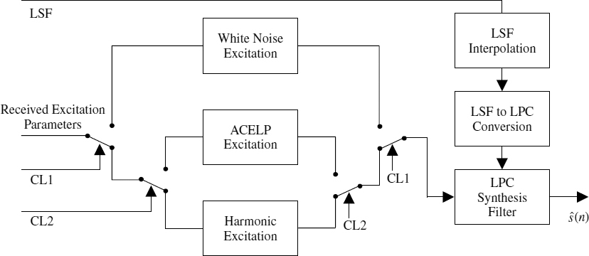
Figure 9.25 Block diagram of the hybrid decoder

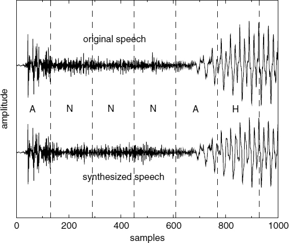
Figure 9.26 Synthesized speech and classification: A (ACELP), H (harmonic), and N (noise excitation)

9.8 Performance Evaluation

The hybrid coder [26] described above has been tested to evaluate its performance. The major tasks were developing a reliable classification technique and preserving the phase continuity when switching between the coding modes. The classification algorithm is tested using 64 seconds of modified IRS-filtered speech, by comparing the mode decision against manually-classified waveforms. Eight English sentence pairs uttered by four male and four female speakers, taken from the Nippon Telegraph and Telephone [50] speech database are used as the test material. The silence segments are excluded from the analysis and synthesized using white-noise excitation. The initial classification detects all the voiced frames. Therefore the worst possible classification error, i.e. classifying a voiced frame as unvoiced, is eliminated. More than 90% of the unvoiced frames are also detected and the rest of the unvoiced frames are misclassified as voiced. This bias towards voiced is preferable to misclassifying voiced frames as unvoiced, since the misclassified unvoiced frames will be classified as ACELP by the secondary classification, while a misclassified voiced frame will be synthesized using white-noise excitation. The plosive detection algorithm detects all the plosives in the unvoiced frames and does not misclassify other unvoiced frames as plosives.

The transition frames are manually marked by observing the waveforms, in order to test the closed-loop transition detection algorithm. Speech frames which have irregular pitch periods and show large variations in the energy are identified as transitions. The closed-loop transition detection classifies the frames already classified as voiced by the initial classification into transitory and harmonic. Consequently, all the frames classified as voiced by the initial classification are included in the test and the unvoiced frames that are classified as voiced are marked as transitions, since they are expected to be synthesized using ACELP. When testing the transition detection algorithm, the use of waveform coding for pitch periods longer than 100 samples is not activated. The transition detection algorithm detects more than 90% of the transition frames and the rest of the transitions are classified as harmonic frames. It also detects more than 90% of the harmonic frames and the rest of the stationary voiced frames are classified as transitions.

Misclassifications may restrict the maximization of the speech quality because of not choosing the best coding algorithm. However misclassifications of the secondary classification do not degrade the speech quality, due to its closed-loop nature. A misclassification of a stationary voiced segment as a transition indicates a harmonic parameter estimation error and such frames are synthesized using ACELP, perhaps a better solution than synthesizing with the inaccurate harmonic parameters. A misclassification of a transition as stationary voiced indicates that the harmonic mode is capable of synthesizing the particular transitory frame. This may be possible at some transitions, particularly offsets, which usually have a steady pitch contour and a smooth energy variation, where the harmonic interpolation model can fit in.

The phase continuity is tested by listening to the synthesized speech, without introducing quantization. The tests verify the validity of the hybrid model and there are no perceptible discontinuities. The speech synthesized also indicates the upper bound of the quality achievable by the designed hybrid model. An informal listening test was conducted using 128 kb/s linear pulse code modulation (PCM), which is the best narrow-band speech quality, and 8 kb/s ITU G.729, a toll-quality speech coder, as the reference coders [26]. The speech material used for the test consists of eight sentences, four from male and four from female talkers, filtered by the modified IRS filter and a pair of headphones was used to conduct the test. Twelve listeners were asked to indicate their preferences for the randomized pairs of synthesized speech. Both experienced and inexperienced listeners participated in the test. The subjective test results are shown in Tables 9.1 and 9.2. As indicated by these results, the unquantized hybrid model performs better than G.729 and worse than 128 kb/s linear PCM. Therefore the quality of the unquantized hybrid model can be classified as being higher than toll quality and lower than transparent quality. In general, the speech encoded and decoded with unquantized hybrid coder model parameters does not sound too different from the original speech material. The perceived speech quality shows only a slight degradation, even after quantizing the harmonic mode parameters at 4 kb/s and white-noise excitation at 1.5 kb/s, with unquantized transitions (at 128 kb/s linear PCM). The hybrid coder achieves toll quality when transitions are quantized with 6 kb/s ACELP.

Table 9.1 Unquantized hybrid model vs 128 kb/s linear PCM

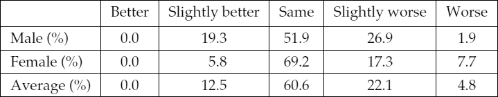
Table 9.2 Unquantized hybrid model vs 8 kb/s G.729

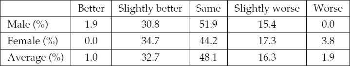
9.9 Quantization Issues of Hybrid Coder Parameters

9.9.1 Introduction

The above hybrid speech-coding model can be adopted for various applications with different quality requirements by quantizing the model parameters at different bit-rates. For applications which support variable bit rates, the model parameters of different modes may be quantized at different bit-rates, allocating the minimum number of bits required for each mode to maintain adequate quality.

In the example, here the LPC parameters are common for all the modes, and quantized using a fixed number of bits per frame. This is advantageous under noisy channel conditions, since the LPC parameters can be decoded correctly even when the mode bits are in error. The LPC parameters are quantized in the LSF domain using a multi-stage vector quantifier (MSVQ), with a first order moving average (MA) prediction [37]. Having quantized the LSFs, the excitation of the three modes are quantized differently.

9.9.2 Unvoiced Excitation Quantization

The hybrid coding algorithm synthesizes unvoiced speech using scaled white Gaussian noise as the LPC excitation. Therefore, only a gain term is required in addition to the LPC parameters to synthesize unvoiced speech. In order to synthesize the unvoiced plosives with adequate quality, the gain term should be updated at least every 5 ms. However listening tests show that synthesizing plosives using ACELP gives better perceptual quality. Therefore the plosives are synthesized using ACELP. The energy of the fricatives does not show rapid fluctuations and updating at the frame rate of every 20 ms is adequate to synthesize high-quality unvoiced fricatives.

The unvoiced gain g_uv is quantized using a logarithmic scalar quantizer. The quantized unvoiced gain g_uvi is given by,

where N is the number of quantizer levels, g_max, defines the upper limit of g_uvi, and k is a constant which controls the gradient of the exponential function. All the g_uv values larger than g_max are clipped at g_max. The constant k is set as 16 and 32 quantizer levels were sufficient to produce high quality unvoiced speech. Hence five bits are required to transmit the quantized unvoiced gain, g_uvi. Figure 9.27 depicts a typical plot of the unvoiced gain quantizer levels where the maximum g_max = 904.

9.9.3 Harmonic Excitation Quantization

The stationary voiced speech segments are synthesized using the synchronized harmonic excitation model described earlier. The model parameters of the harmonic excitation with SWPM are pitch period, pitch pulse location (PPL), pitch pulse shape (PPS), harmonic amplitudes, and gain. The AbS transition detection algorithm synthesizes the harmonic excitation using SWPM at the encoder to evaluate the suitability of the harmonic mode. Therefore, quantized or unquantized harmonic parameters may be used for the transition detection at the encoder. Generally, AbS algorithms include the quantization in the error minimization loop, so that the quantization noise is also accounted for in the parameter estimation process. However in this case, the solution is not straightforward, since the decision is between two modes, rather than the best set of parameters of a unimodal coder. One solution to this problem is to perform a full closed-loop mode decision with quantized parameters, i.e. synthesizing the speech frames with all the modes and selecting the best mode. A weighting factor may be required in the mode selection process, since the harmonic excitation with SWPM may give superior perceptual quality even with a slightly lower SNR compared to ACELP. However such a solution is computationally demanding, since ACELP excitation should be computed for all the frames, excluding the silence and unvoiced frames. Furthermore, defining a suitable weighting factor which reflects the perceptual quality is a difficult task.

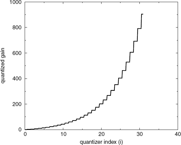
Figure 9.27 Unvoiced gain quantizer levels

A more practical solution is to decide the inclusion of the harmonic parameter quantization in the mode decision loop based on ACELP bit rate. The inclusion of the harmonic quantization in the closed-loop mode decision increases the number of ACELP mode frames. However, occasionally switching to ACELP between harmonic frames may degrade the perceptual quality, when the bit rate of the ACELP mode is below 8kb/s, due to the sudden discontinuities introduced in the voiced harmonics. In general, ACELP operating at 8 kb/s or higher is capable of synthesizing perceptually-superior speech compared to harmonic coding (with no phase transmission), even at the stationary voiced segments. Therefore the harmonic quantization can be included in the closed-loop mode decision without worrying about the quality of ACELP coded frames between the harmonic frames (except, of course, the bit rate will be higher). However when the bit rate of ACELP mode is low, the quantization noise becomes audible; hence, trying to eliminate the quantization noise of the harmonic mode by switching to ACELP mode does not improve the perceptual quality. Therefore, in all the tests described here, harmonic parameter quantization is not included in the transition detection loop.

The sensitivity of AbS transition detection is different for each parameter. The sensitivity is high for the pitch period and PPL. Changes in these parameters dramatically reduce the cross-correlation of the original and the synthesized speech, due to the resulting time shifts. The spectral amplitudes and the LPC parameters are least sensitive. In fact, quantized and unquantized LPC parameters both produced the same classification decisions for the test speech material. The LPC memory locations of the transition detection algorithm are initialized for each frame with the memory locations of the LPC synthesis filter. This avoids drifting the LPC synthesis filter of the transition detection algorithm from the synthesized speech.

Pitch Quantization

The pitch period, τ, is quantized using a nonlinear scalar quantizer, reflecting the high sensitivity of the human ear to the pitch deviations at shorter pitch periods. A logarithmic scale is used for the pitch values from 16 to 60 samples and a linear scale is used for the pitch values from 60 to 160 samples (see Figure 9.28). The quantized pitch τ_i is given by,

where τ_min is 16, τ_max is 160, τ₀ is 60, N₀ is 156, and N is 256. Therefore eight bits are required to transmit the quantized pitch period.

Pitch Pulse Location Quantization

The pitch pulse location (PPL) is the location of the pitch pulse closest to the centre of the analysis frame. PPL may be defined as the distance to the pitch pulse concerned from the centre of the analysis frame, measured in samples. Assuming that the maximum possible pitch is 160 samples, PPL varies between −80 and 80. However the pitch pulse location may be normalized with respect to the pitch so that the PPL varies between −0.5 and 0.5. Normalization of the PPL with respect to the pitch ensures the efficient use of quantizer dynamic range regardless of the pitch.

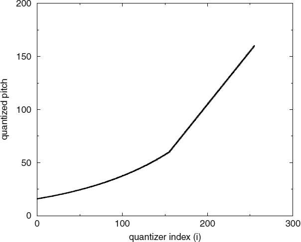
Figure 9.28 Pitch quantizer levels

The accuracy of the PPL is more important when it is close to the centre of the analysis frames or the synthesis frame boundaries, i.e. PPL values close to zero. This is due to the fact that the mode changes between ACELP and harmonic excitation may take place at the synthesis frame boundaries. Preserving the continuity of the high-energy pitch pulses occurring at or close to the switching frame boundaries is essential to eliminate audible switching artifacts. Therefore the normalized PPL is quantized using a logarithmic scale, quantizing the PPL values close to zero more accurately. The quantized PPL, t_i is given by,

where N is the number of quantizer levels and k is a constant that controls the gradient of the exponential function. The constant k is set to 0.125, and 128 quantizer levels are sufficient to eliminate audible switching artifacts. Hence seven bits are required to transmit the quantized normalized PPL. PPL is normalized using the quantized pitch so that the decoder can denormalize the received PPL value accurately. Figure 9.29 depicts a plot of the normalized PPL quantizer levels.

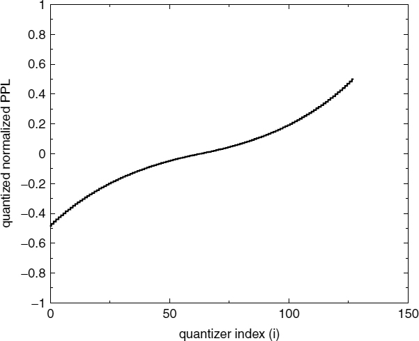
Figure 9.29 PPL quantizer levels

Pitch Pulse Shape Quantization

Large variations in the PPS introduces a reverberant character into the synthesized speech, regardless of the PPS value. Therefore, in terms of the perceptual quality, all the PPS values are equally important and a linear quantizer is employed to quantize the PPS using 16 values. The quantized PPS, θ_i, is given by,

where N, the number of quantizer levels, is 16 and four bits are required to quantize PPS.

Harmonic Amplitude Quantization

Harmonic amplitudes of the LPC residual are quantized using Switched Predictive Mel-scale-based Vector Quantization (SP-MVQ) [51]. SP-MVQ (see block diagram in Figure 9.30) converts the variable-dimension spectral-amplitude vectors into fixed-dimension vectors by warping the frequency axis using a logarithmic scale. The warping process emphasizes the low frequencies, taking into account the perceptual preferences of the human auditory system. The fixed dimension spectral vector, , is decomposed into a predicted vector, , and a prediction residual vector, , as follows:

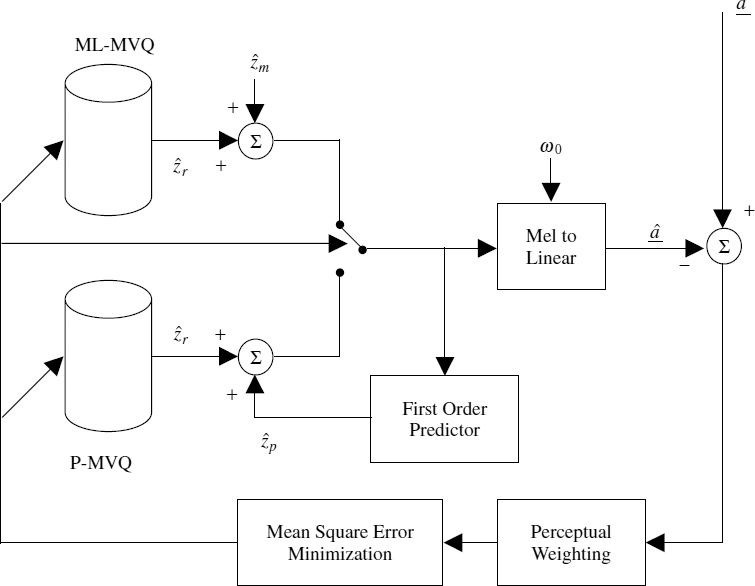
Figure 9.30 Block diagram of SP-MVQ

where the predicted vector, , is obtained using a first-order autoregressive method, given by,

where is the most recently quantized , is the mean vector, and Φ denotes a diagonal matrix of prediction coefficients. The prediction residual, is quantized using a typical vector quantizer such as MSVQ [52]. The quantization becomes memoryless Mel-scale-based vector quantization (ML-MVQ) if all the prediction coefficients are zero, and autoregressive predictive MVQ (P-MVQ) otherwise. The predictive scheme is effective in stationary regions, and may increase spectral distortion at the transitions; therefore, a switching scheme is introduced to switch between P-MVQ and ML-MVQ. The decision between P-MVQ and ML-MVQ is made using AbS techniques and based on a weighted spectral-distortion measure. Therefore the quantization scheme is called switched predictive Mel-scale-based vector quantization (SP-MVQ). Moreover, the switching scheme restricts error propagation under noisy channel conditions.

SP-MVQ quantizes spectral amplitudes every 10 ms using 14 bits. The harmonic analysis/synthesis scheme described estimates the harmonic parameters every 20 ms. However there are sufficient bits for the allocation of 28 bits per 20 ms frame for spectral amplitudes at 4 kb/s (see Table 9.5). Therefore the harmonic analysis/synthesis scheme is modified to update the spectral amplitudes every 10 ms. However the pitch is transmitted only every 20 ms, and linearly interpolated to compute the number of harmonics corresponding to the centre of the synthesis frame or the first subframe, at the decoder. The spectral amplitude quantization uses the quantized (second subframe) or quantized and interpolated (first subframe) pitch to compute the number of harmonics, in order to ensure the correct dequantization of the spectral amplitude vectors. In the spectral amplitude quantization of the first subframe, if the actual number of harmonics is greater than the computed number of harmonics by interpolation, the higher harmonics are ignored. If the actual number of harmonics is less than the computed number of harmonics by interpolation, the amplitude vector is zero-padded. Usually the pitch values of the stationary voiced segments are fairly unchanged and linear interpolation of the number of harmonics gives a good approximation.

Harmonic Gain Quantization

The spectral amplitude vectors are normalized before the quantization, in order to improve the dynamic range. The shape components of the vectors are quantized using SP-MVQ, as described above, and the gain component is scalar quantized.

The normalized amplitude, a_kn, of the k^th harmonic is given by,

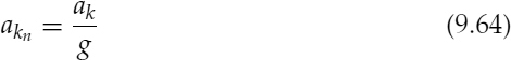
where a_k is the spectral amplitude estimated for the k^th harmonic and g is the normalization factor, given by,

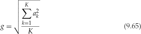
where K is the total number of harmonics. Normalization factor of the second subframe, g₂, is quantized using a logarithmic scale, given by,

where k is eight (which controls the gradient of the exponential function), N (the number of quantizer levels) is 32, i.e. five bits are required to quantize the gain of the second subframe, and g_max and g_min are the maximum and minimum possible quantized normalization factors, respectively. The gain values beyond g_max and g_min are clipped by the quantizer. The term g_min is introduced in equation (9.66), because only the stationary voiced segments are synthesized using the harmonic excitation and the minimum gain is nonzero.

The normalization factor of the first subframe, g₁, is differentially quantized with respect to the mean of the adjacent two quantized g₂ values, as follows:

where g₂₋₁ is the gain of the second subframe of the previous frame, i.e. the previous g₂, and δ is quantized using three bits. Finally the spectral amplitude vectors are denormalized by multiplying with the quantized normalization factors.

Onset Harmonic Parameter Quantization

The harmonic synthesis process interpolates the parameters between the synthesis frame boundaries. However, at the onsets, when switching from waveform-coding mode, the harmonic parameters of the initial synthesis frame boundary are not directly available. The pitch, PPL, and PPS are estimated, as described in Section 9.5.4, and quantized as described in the preceding sections.

The spectral amplitudes of the ACELP excitation signal used before the harmonic mode are estimated by windowing it using an asymmetric window function given by,

where n₁ is 140 and n₂ is 20. The asymmetric window function emphasizes the excitation signal close to the switching frame boundary.

The spectral amplitude vector of the windowed ACELP excitation signal is obtained by peak-picking of the magnitude spectrum, using the received pitch value for the harmonic frame. The rms normalization factor of the estimated spectral vector is used as g₂₋₁ of the harmonic frame. The amplitude quantization memory, is initialized by quantizing the normalized shape vector, while forcing SP-MVQ to use memoryless quantization.

9.9.4 Quantization of ACELP Excitation at Transitions

The transitions are quantized using algebraic code excited linear prediction (ACELP). The pulse innovation of ACELP is capable of synthesizing highly nonstationary transitions. The long term prediction (LTP) is not very efficient at the onsets, since the LTP memory buffer has no information regarding the onsets. However LTP is employed, because it reduces the sparse excitation artifacts [39] and synthesizes a significant amount of the excitation at the offsets. Moreover, at the resonance offsets, where the gain of the excitation signal is small, the LTP gain acts as an adaptive gain term and compensates for an inadequate gain quantization dynamic range of the innovation pulses. Multi-tap and fractional delay LTP filters [53] are useful only for stationary voiced segments, consequently, only integer delays and single-tap filters are used to encode transitions.

The LTP gain is close to unity during the stationary voiced segments. However at the transitions, LTP gain shows large variations, due to the large variations in the speech energy. Therefore the LTP gain is quantized using a larger dynamic range. A drawback in allowing gain values larger than unity is that the LTP filter may become unstable under erroneous channel conditions. The high-energy pulses of plosives are synthesized using only the innovation sequence of ACELP. However the plosives are not classified as a separate mode; instead, when a plosive is detected, the LTP gain is forced to be zero.

9.10 Variable Bit Rate Coding

When using a 4 kb/s harmonic coder for steady state voiced segments and unvoiced segments quantized at 1.5kb/s (as detailed in Table 9.5) with unquantized transitions, the synthesized speech quality shows only a slight degradation when compared with using the unquantized model parameters, which is nearly transparent. The quality versus the bit-rate limitation of this hybrid coder is therefore dependent on transition quantization by ACELP. Informal listening tests show that quantizing the transitions at 6kb/s is sufficient to achieve toll quality. Three versions of the coder are tested and compared with standard coders by quantizing the transitions at 4, 6 and 8kb/s.

9.10.1 Transition Quantization with 4 kb/s ACELP

The 4kb/s version uses 10ms subframes. For each subframe the LTP delay, LTP gain, locations, signs, and the gain of two innovation pulses are transmitted. The innovation gain terms of the two subframes are normalized with respect to the quantized rms energy of the speech signal and the normalization factor is transmitted for each 20 ms frame. The normalization reduces the dynamic range required to quantize the innovation sequence gain. Table 9.5 shows the bit allocation of the 4kb/s ACELP parameters. The LTP delay range is from 20 to 147, and only integer delays are allowed, needing seven bits for the index. The LTP gain is quantized using four bits (see Table 9.3). The two innovation pulses cover only the first 64 locations of each 80-sample subframe. Each pulse is chosen from 32 possible locations, either even or odd, and five bits are required to transmit the location. The sign of each pulse is transmitted using one bit. The pulse gain and the common normalization factor of the frame are quantized using three bits each (see Table 9.4).

9.10.2 Transition Quantization with 6 kb/s ACELP

The 6 kb/s version uses 5 ms subframes. For each subframe the LTP delay, LTP gain, locations, signs, and the gain of two innovation pulses are transmitted. The pulse gain terms of the four subframes are normalized with respect to the quantized rms energy of the speech signal and the normalization factor is transmitted for each 20 ms frame. Table 9.5 shows the bit allocation of the 6 kb/s ACELP parameters. The LTP delay and gain are quantized in the same way to the 4kb/s version, using seven bits and four bits respectively.

The two innovation pulses cover only the first 32 locations of each 40-sample subframe. Each pulse is chosen from 16 possible locations, either even or odd, and four bits are required to transmit the location. The signs of the two pulses are forced to be opposite in the error minimization process, hence only the sign of the first pulse is transmitted, using one bit. The pulse gain and the common normalization factor of the frame are quantized using three bits each (see Table 9.4).

Table 9.3 LTP Gain quantizer table

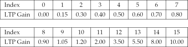
Table 9.4 Innovation pulse gain quantizer table

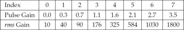
Table 9.5 Bit allocation for a 20 ms frame

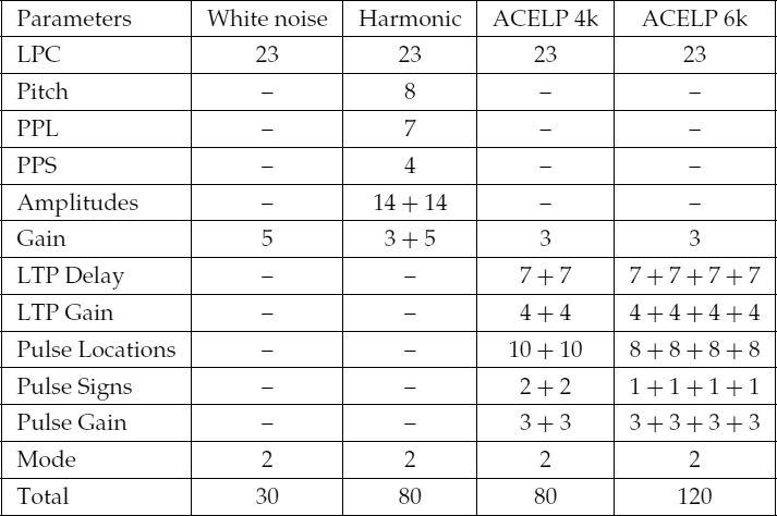
9.10.3 Transition Quantization with 8 kb/s ACELP

The 8kb/s version uses 5ms sub frames. For each subframe the LTP delay, LTP gain, locations, signs, and the gain of four innovation pulses are transmitted. The pulse gain terms of the four subframes are normalized with respect to the quantized rms energy of the speech signal and the normalization factor is transmitted for each 20 ms frame. Table 9.8 shows the bit allocation of the 8 kb/s ACELP parameters. The LTP delay and gain are quantized in the same way as the 4 kb/s version, using seven bits and four bits, respectively.

The locations and the signs of the four pulses are shown in Table 9.6. The pulse gain of each subframe is quantized using four bits, as shown in Table 9.7. The common normalization factor, i.e. the rms energy of the original speech signal, in each frame is logarithmically quantized using seven bits, and the quantized value, g_rmsi, is given by,

Table 9.6 Structure of the 17-bit algebraic codebook

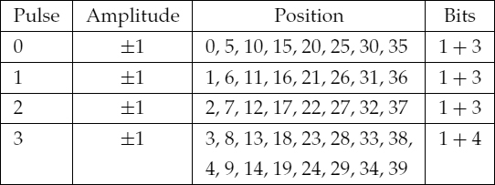
Table 9.7 Innovation pulse gain quantizer table for 8 kb/s ACELP

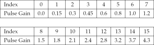
Table 9.8 Bit allocation of 8 kb/s ACELP for a 20 ms frame

Parameters	ACELP 8k
LPC	23
Gain	7
LTP Delay	7+7+7+7
LTP Gain	4+4+4+4
Pulse Locations	13 + 13 + 13 + 13
Pulse signs	4+4+4+4
Pulse Gain	4+4+4+4
Mode	2
Total	160

Where k (a constant which controls the gradient of the exponential function) is 80, N (the number of quantizer levels) is 128, and g_max and g_min are 2720.5 and 0.5 respectively.

9.10.4 Comparison

Three informal listening tests were conducted to assess the speech quality of the hybrid coder, with transitions quantized at 4 kb/s, 6 kb/s, and 8 kb/s. The synthesized speech was compared against that from 5.3kb/s ITU G.723.1, 6.3 kb/s ITU G.723.1, and 8 kb/s ITU G.729 coders. In all the tests, stationary voiced segments were quantized at 4 kb/s, and silence and unvoiced segments are quantized at 1.5kb/s. The speech material used for each test consists of eight sentences, four from male and four from female talkers, filtered by modified IRS filter; a pair of headphones was used to conduct the test. Twelve listeners were asked to indicate their preferences for randomized pairs of synthesized speech. Both experienced and inexperienced listeners participated in the test. The subjective test results are shown in Tables 9.9, 9.10, and 9.11.

For the speech material used in the subjective tests, after discarding the silence frames, about 64% of the frames used harmonic excitation, 22% used ACELP, and 14% used white-noise excitation. The 4kb/s, 6 kb/s, and 8 kb/s ACELP mode hybrid coders give average bit-rates of 3.65 kb/s, 4.1 kb/s, and 4.53 kb/s, respectively. The 4 kb/s ACELP version performs slightly better than G.723.1 at 5.3 kb/s. The 6 kb/s ACELP version achieves similar quality to G.723.1 at 6.3 kb/s. The quality of the 8 kb/s ACELP version is also similar to G.729 at 8 kb/s, with an overall average bit rate of 4.53 kb/s.

Table 9.9 4 kb/s ACELP hybrid vs 5.3 kb/s G.723.1

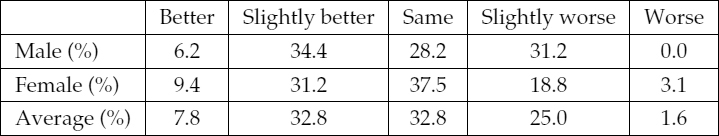
Table 9.10 6 kb/s ACELP hybrid vs 6.3 kb/s G.723.1

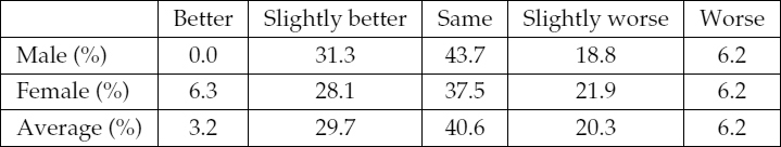
Table 9.11 8 kb/s ACELP hybrid vs 8 kb/s G.729

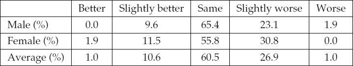
9.11 Acoustic Noise and Channel Error Performance

Robustness to background noise and channel errors is an important factor for any practical speech-coding algorithm. The speech coders designed for mobile and military communication applications frequently encounter acoustic noise and channel errors. The background noise may be suppressed before the encoding process using a noise preprocessor [54]. However, this involves additional complexity and delay, which may not be desirable for mobile communication applications. Therefore the speech-coding algorithms are expected to produce intelligible synthetic speech even in the presence of background noise. Generally, AbS coders perform better than parametric coders under noisy background conditions. This inherent robustness of AbS coders is due to their waveform-matching process. The error minimization process attempts to synthesize the input waveform regardless of its contents. The model parameters estimated by the parametric coders may not be accurate when the input speech signal is corrupted with noise. Inaccurate model parameters may severely degrade the synthetic speech of a parametric coder.

Channel errors are usually divided into two classes: random errors and burst errors. A speech-coding algorithm should provide a reasonable output even if a small proportion of the received bit stream is incorrect due to random bit errors. Robustness against random channel errors can be increased by means of index assignment algorithms [55, 56], through proper quantizer design, and by adding redundancy into the transmitted information [57, 58, 59]. Unequal error protection techniques may be applied to provide a higher degree of protection to the most sensitive bits. For example, in CELP coders, the spectral envelope parameters are the most sensitive to errors, followed by the fixed codebook gain, the adaptive codebook index, the adaptive codebook gain, the sign of the fixed codebook gain, and the fixed codebook index [60]. In the case of sinusoidal coders, the gain is the most sensitive to errors, followed by the voicing, the pitch, the spectral envelope parameters, and the spectral amplitudes [61].

In the case of burst errors, error detection schemes are used to classify each frame of received bits as usable or unusable. A similar problem encountered in packet voice communication systems is lost packets due to transmission impairments and excessive delays. In order to reduce the annoying artifacts due to lost frames, concealment techniques based on waveform substitution can be used [62]. The burst errors may also be converted to occur in a more random fashion using interleaving techniques. The performance issues specific to a hybrid coding algorithm are the robustness of the classification algorithm under acoustic noise and the channel bit error performance of the coding mode; otherwise, the performance of hybrid coders will be similar to either ACELP or harmonic coding.

9.11.1 Performance Under Acoustic Noise

The classification algorithm was tested using 64 seconds of male and female speech corrupted with either babble or vehicular noise. The SNR of the corrupted speech is 10 dB.

Figure 9.31 depicts the classification of the female speech. The initial classification declares only the strongly-unvoiced segments as unvoiced and all the other frames are left to be encoded using either ACELP or harmonic excitation (compare Figures 9.31b and 9.32b). The weakly-unvoiced segments which have lower energy than the noise level are not detected as unvoiced. When corrupted with babble or vehicular noise, the silence and the low-energy unvoiced segments do not have the properties of unvoiced speech. It can be seen that the energy of the noise component is comparable with unvoiced speech and it has a significant low-frequency component (see Figure 9.35a). This is expected since babble noise is essentially attenuated and superimposed speech components. Figure 9.33 shows the classification of the male speech and Figure 9.34 shows the corresponding clean speech segments.

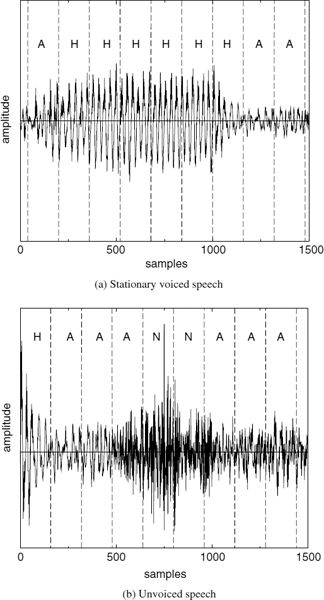
Figure 9.31 Classification of female speech corrupted by babble noise (10dBSNR): A (ACELP), H (harmonic), and N (noise excitation)

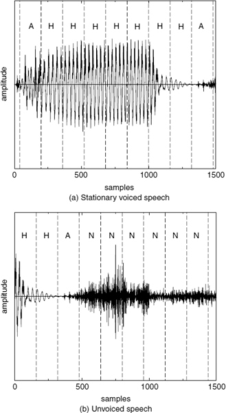
Figure 9.32 Classification of clean speech corresponding to Figure 9.31

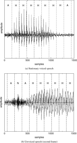
Figure 9.33 Classification of male speech corrupted by babble noise (10dB SNR): A (ACELP), H (harmonic), and N (noise excitation)

The secondary classification performs very similarly under the clean speech conditions, except for the occasional classification of frames as ACELP, which were originally classified as harmonic under the clean speech conditions (compare Figures 9.31a and 9.32a). This is due to the inability of the harmonic model to adequately synthesize the corrupted signal and the model parameter estimation errors. Therefore, in general, in the presence of acoustic noise the speech classification algorithm declares more frames as ACELP. These include the silence frames of the original clean speech, unvoiced segments with lower energy than the noise level, and the stationary voiced frames with parameter estimation and harmonic modelling difficulties.

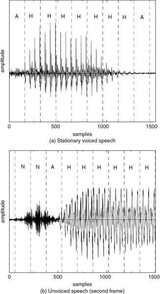
Figure 9.34 Classification of clean speech corresponding to Figure 9.33

Neither white-noise excitation nor harmonic excitation is suitable for synthesizing the background noise. The spectra of babble and vehicular noise are not white, even after discarding the spectral envelope. synthesizing them using white-noise excitation will degrade the perceptual quality by introducing an unnaturally noisy background. Therefore, in fact, the classification algorithm detects the most suitable mode, i.e. ACELP, to synthesize back-ground noise. However the drawback is a high average bit-rate, which may be reduced by using a robust voice activity detection (VAD) algorithm and comfort noise generation at the decoder end [9].

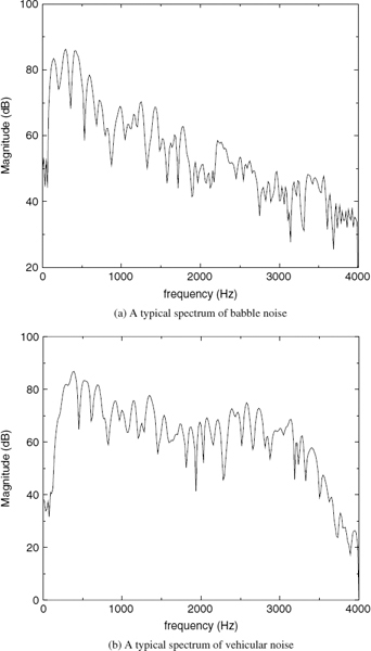
Figure 9.35 Typical acoustic noise spectra

The correct classification of the stationary voiced segments as harmonic mode under noisy background conditions confirms the robustness of SWPM, since the AbS classification algorithm synthesizes speech using SWPM. There-fore, it can be concluded that the pitch pulse location (PPL) and the pitch pulse shape (PPS) detection algorithms described in Section 9.4 perform well under noisy background conditions.

An informal listening test was conducted to compare the speech quality of the hybrid coder under noisy background conditions with white noise, harmonic excitation, and ACELP quantized at 1.5 kb/s, 4kb/s, and 6kb/s, as discussed before. The synthesized speech was compared against the same noisy speech files synthesized using the 6.3 kb/s ITU G.723.1 coder. The speech material used for each test consists of eight sentences, four from male and four from female talkers, four corrupted with vehicular noise and four corrupted with babble noise (10 dB SNR); a pair of headphones was used to conduct the test. Twelve listeners were asked to indicate their preferences for the randomized pairs of synthesized speech. Both experienced and inexperienced listeners were participated in the test. The test results are shown in Table 9.12.

The informal listening test shows a clear preference for the 6.3 kb/s ITU G.723.1 coder. It was found that this is due to the metallic character of the stationary voiced speech synthesized by the harmonic excitation: it is cleaner, however, there is a pronounced metallic character. The test confirms that the listeners prefer more natural-sounding, noisy speech rather than metallic speech.

The metallic character is not so pronounced in noisy speech synthesized using a split-band LPC (SB-LPC) harmonic coder [4]. The SB-LPC coder divides the speech spectrum into two bands using a voicing frequency marker, where the upper band is declared unvoiced, and synthesized using a filtered noise excitation. For clean stationary voiced speech, most of the spectrum is declared voiced. However in the case of stationary voiced segments of noisy speech, some frequency bands are declared unvoiced. Therefore the voicing decision of SB-LPC reduces quality, synthesizing metallic sounds under noisy background conditions. The harmonic excitation model described in Section 9.5.1 was designed to synthesize stationary voiced segments and the complete spectrum is synthesized using harmonically related sinusoids. Under noisy background conditions, there are strong spectral components which are not related to the fundamental frequency of the speech. These noise components change the harmonic amplitudes and are perceived as metallic sounds in harmonically synthesized speech (see Figure 9.36). Introducing a voicing frequency marker for the harmonic excitation, similar to SB-LPC, improves the speech quality of the hybrid coder, especially in noisy back-ground conditions. The hybrid coding algorithm described has three modes, and two bits are allocated to transmit the mode. Therefore an additional mode may be added to further improve the speech quality. The quality of speech corrupted by acoustic noise can be improved by using the additional mode as another harmonic mode with a constant voicing frequency marker, e.g. 80% of the spectrum is voiced. Figure 9.37 depicts the spectrum of speech corrupted with babble noise (10 dB SNR) and the spectrum of the synthesized speech, with 80% of the spectrum declared voiced and the remaining high frequency components synthesized using filtered and scaled Gaussian noise.

Table 9.12 Hybrid vs 6.3 kb/s G.723.1 for noisy speech

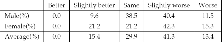
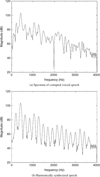
Figure 9.36 Speech corrupted with babble noise (10dB SNR)

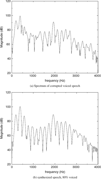
Figure 9.37 Speech corrupted with babble noise (10dB SNR)

Table 9.13 Hybrid vs 6.3 kb/s G.723.1 for noisy speech

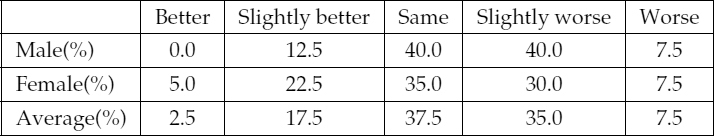
The same informal listening test was conducted to compare the speech quality. The informal test results are shown in Table 9.13. Comparing with the results shown in Table 9.12, the introduction of the harmonic voicing significantly improves the performance under background noise which indicates that there is still some room to retune the harmonic coder for the hybrid coding operation. The same is perhaps true for ACELP, and it should be designed specifically for hybrid operation.

9.11.2 Performance Under Channel Errors

The inherent robustness of the hybrid coder to mode bit errors was tested by simulating all the possible mode errors. The hybrid coder has three modes, hence there are six possible mode errors, i.e. each mode may be erroneously decoded with the other two modes. The bit stream of the hybrid coder is shown in Tables 9.14 and 9.15. For each parameter, the most significant bit (MSB) is transmitted first. When erroneously decoding a lower-rate mode as a higher-rate mode, e.g. decoding a white-noise excitation frame as harmonic, the remaining bits are set to 1. Simulations show that setting the remaining bits to 1 has the worst effect, since the higher indices are mapped to the higher-energy levels in the gain quantizers. Using the LTP gain quantizer shown in Table 9.3 results in blasts when the white noise or harmonic frames are erroneously decoded as ACELP. Therefore the maximum LTP gain is limited to 1.2.

All the modes quantize the LSFs using 23 bits, consequently they are transmitted using the same bits. Therefore the LSFs are independent of the mode and the mode bit errors can only affect the excitation parameters. This is particularly attractive for the LSF interpolation and quantization with first-order moving average prediction. The most significant bits of the gain parameters are also transmitted using the same bits. However the gain of each mode is estimated using different criteria. Hence the gain quantizers of each mode have different dynamic ranges, and mode errors affect the dequantization of the gain.

Table 9.14 Transmission bit stream of the hybrid coder

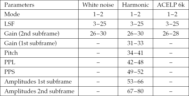
Table 9.15 Bit stream of 6 kb/s ACELP subframes

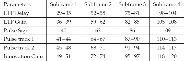
White Noise Excitation Mode Errors

Figure 9.38 illustrates erroneous decoding of white-noise excitation frames as harmonic and ACELP. It shows that the errors are contained within the frames which have mode errors. This is because the decoder does not interpolate the unvoiced gain at switching. The present gain is used to synthesize the entire frame when switched from a different mode. However if the next frame after decoding a noise excitation frame as ACELP is also ACELP, the LTP memory propagates the errors, similar to the error propagation of CELP coders [60]. The hybrid coding algorithm has the advantage of limiting the error propagation, by switching to a different mode, which also refreshes the LTP memory.

Harmonic Mode Errors

Figure 9.39 illustrates erroneous decoding of harmonic excitation frames as unvoiced and ACELP. It shows that the errors are contained within the frames which have mode errors. This is because the decoder reinitializes the harmonic excitation memories when switched from a different mode, and use of the previous excitation vector is minimized. However if the next frame after decoding a harmonic excitation frame as unvoiced is also unvoiced, the unvoiced overlap and add process spreads the incorrect gain into the next frame.

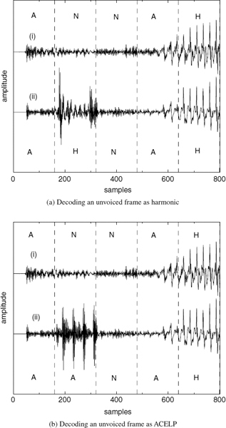
Figure 9.38 Erroneous decoding of white-noise excitation frames: (i) Original speech, (ii) synthesized speech: A (ACELP), H (harmonic), and N (noise excitation)

ACELP Mode Errors

Figure 9.40 illustrates erroneous decoding of ACELP frames as unvoiced and harmonic. In Figure 9.40a the error is contained within the frame which has the mode error. For the next frame the harmonic mode reinitializes the excitation memories. However in Figure 9.40b, the next frame after decoding an ACELP frame as harmonic is also harmonic. Hence, the error propagates into the next frame, due to the harmonic interpolation process.

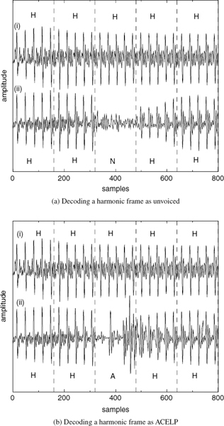
Figure 9.39 Erroneous decoding of harmonic excitation frames, (i) Original speech, (ii) synthesized speech: A (ACELP), H (harmonic), and N (noise excitation)

The LPC filter may propagate the errors, when the filter response is highly resonant. However the bandwidth expansion of the LPC coefficients ensures that the LPC impulse response dies away more quickly. Therefore all the mode errors are localized and the output does not become unstable in the presence of mode errors. This is mainly due to the independent memory initialization procedures of the coding algorithm when switching between the modes. The white-noise excitation mode always sets the previous gain equal to the present one when switched from a different mode. The harmonic excitation mostly depends on the received harmonic parameters when switched from a different mode; only the amplitude quantizer memories are initialized using the previous excitation vector. The LTP buffer is refreshed, regardless of the mode, with the latest excitation vector.

9.11.3 Performance Improvement Under Channel Errors

During the experiments described in the preceding sections, the robustness to mode-bit errors was improved by limiting the LTP gain to 1.2 and using the same set of bits to transmit the LSFs of all the modes. The encoder and the decoder cannot synchronize the random number generators at the presence of mode-bit errors. This affects the performance of the LTP when switched from white-noise excitation. However the exact content of the white-noise excitation has no significance and can be represented by any noise excitation vector. Therefore, the performance of the LTP was also improved by always reinitializing the LTP buffer to a fixed stored noise excitation vector when switching to ACELP from the white-noise excitation.

The robustness to mode-bit errors can be further improved by using error detection and correction techniques. If a mode error is only detected and not corrected, the concealment techniques based on waveform substitution can be used to reduce the resulting annoying artifacts [62]. The decoded parameters and the synthesized waveform may also be used to detect mode errors. As can be seen in Figures 9.38, 9.39, and 9.40, mode errors generally result in sudden changes in the waveform shape and the signal level, which are unusual for speech signals. Moreover certain mode patterns are more common than the others, e.g. for many speech utterances, ACELP to harmonic and back to ACELP occur, while the silence segments before and after are synthesized with the white-noise excitation. The transition from white noise to harmonic mode is extremely rare, since generally the onsets request ACELP. Consequently in order to assist in detecting mode errors, one can limit the possible switching combinations.

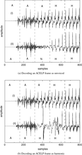
Figure 9.40 Erroneous decoding of ACELP frames, (i) Original speech, (ii) synthesized speech: A (ACELP), H (harmonic), and N (noise excitation)

9.12 Summary

In this chapter the principle techniques behind an advanced hybrid coding algorithm, which integrates harmonic coding and waveform coding, have been presented. The two important design issues are speech classification and, when mode-switching, proper coder synchronization. Provided that these two processing stages are carried out successfully, the quality of speech produced by a hybrid coding method is of good to toll quality at around 3.5–5 kb/s (average). Simple informal subjective listening test results confirm that the hybrid model eliminates the limitations of the existing single-model-based coders.

The robustness of the hybrid coding algorithm under acoustic noise and channel error conditions is another important issue which requires significant research effort. The difficulties specific to hybrid coders are the speech classification under background noise, and the mode-bit errors due to random channel errors. Although the classification algorithm is capable of selecting the best mode under noisy background conditions, there is a significant bias towards ACELP in the presence of noise compared to clean speech conditions. This is due to the inability of the white-noise excitation or the harmonic excitation to encode the corrupted signals. The noisy speech synthesized using the harmonic mode sounds metallic, which can be improved by introducing a proper voicing mixture classification when harmonic mode is selected.

The robustness of the hybrid coder to mode errors has been tested by simulating all the possible mode errors. The coder is capable of isolating the mode errors and return to normal decoding almost immediately. This is mainly due to the independent memory reinitialization of the modes when switched from a different mode.

Finally it is important that each element or coding mode of the hybrid model is redesigned with the knowledge that the noise, ACELP and harmonic excitation models will be used during noise (or silence), transitions, and steady state voiced speech parts respectively. In this case the LPC parameters of ACELP and harmonic modes will have different vector quantizer tables which will be trained over transitional and steady state voiced speech only respectively, thus improving the quantization performance. In addition, using the LTP in ACELP mode at the onsets may not be necessary. Instead more pulses with phase spreading may be used to improve quality.

Bibliography

[1] R. J. McAulay and T. F. Quatieri (1995) ‘Sinusoidal coding’, in Speech coding and synthesis by W. B. Kleijn and K. K. Paliwal (Eds), pp. 121–74. Amsterdam: Elsevier Science

[2] R. J. McAulay and T. F. Quatieri (1986) ‘Speech analysis/synthesis based on a sinusoidal representation’, in IEEE Trans. on Acoust., Speech and Signal Processing, 34(4):744–54.

[3] D. Griffin and J. S. Lim (1988) ‘Multiband excitation vocoder’, in IEEE Trans. on Acoust., Speech and Signal Processing, 36(8):1223–35.

[4] I. Atkinson, S. Yeldener, and A. Kondoz (1997) ‘High quality split-band LPC vocoder operating at low bit rates’, in Proc. of Int. Conf. on Acoust., Speech and Signal Processing, pp. 1559–62. May 1997. Munich

[5] R. Salami, C. Laflamme, J.P. Adoul, A. Kataoka, S. Hayashi, T. Moriya, C. Lamblin, D, Massaloux, S. Proust, P. Kroon, and Y. Shoham (1998) ‘Design and description of CS-ACELP: a toll quality 8 kbps speech coder’, in IEEE Trans. Speech and Audio Processing, 6(2):116–30.

[6] C. Laflamme, J.-P. Adoul, H. Su, and S. Morissette (1990) ‘On reducing computational complexity of codebook search through the use of algebraic codes’, in Int. Conf. on Acoust., Speech and Signal Processing, pp. 177–80.

[7] W. B. Kleijn (1993) ‘Encoding speech using prototype waveforms’, in IEEE Trans. Speech and Audio Processing, 1:386–99.

[8] M. Schroeder and B. Atal (1985) ‘Code excited linear prediction (CELP): high quality speech at very low bit rates’, in Proc. of Int. Conf. on Acoust., Speech and Signal Processing, pp. 937–40. Tampa, FL

[9] D. K. Freeman, G. Cosier, C. B. Southcott, and I. Boyd (1989) ‘The voice activity detector for the pan-European digital cellular mobile telephone service’, in Proc. of Int. Conf. on Acoust., Speech and Signal Processing, pp. 369–72.

[10] S. Wang and A. Gersho (1992) ‘Improved phonetically segmented vector excitation coding at 3.4 kbps’, in Proc. of Int. Conf. on Acoust., Speech and Signal Processing, 1:349–352.

[11] T. E. Tremain (1982) ‘The government standard linear predictive coding algorithm: LPC-10’, in Speech Technology, 1:40–9.

[12] P. Kroon and B. Atal (1988) ‘Strategies for improving CELP coders’, in Proc. of Int. Conf. on Acoust., Speech and Signal Processing, 1:151–4.

[13] I. M. Trancoso, L. Almeida, and J. M. Tribolet (1986) ‘A study on the relationships between stochastic and harmonic coding’, in Proc. of Int. Conf. on Acoust., Speech and Signal Processing, pp. 1709–12.

[14] B. S. Atal and S. Singhal (1984) ‘Improving performance of multipulse LPC coders at low bit rates’, in Proc. of Int. Conf. on Acoust., Speech and Signal Processing, pp. 1.3.1–4.

[15] D. L. Thomson and D. P. Prezas (1986) ‘Selective modelling of the LPC residual during unvoiced frames white noise or pulse excitation’, in Proc. of Int. Conf. on Acoust., Speech and Signal Processing, pp. 3087–90.

[16] E. Shlomot, V. Cuperman, and A. Gersho (1998) ‘Combined harmonic and waveform coding of speech at low bit rates’, in Proc. of Int. Conf. on Acoust., Speech and Signal Processing.

[17] E. Shlomot, V. Cuperman, and A. Gersho (1997) ‘Hybrid coding of speech at 4 kbps’, in Proc. IEEE Workshop on Speech Coding for Telecom, pp. 37–8.

[18] J. Stachurski and A. McCree (2000) ‘Combining parametric and waveform-matching coders for low bit-rate speech coding’, in X European Signal Processing Conf.

[19] J. Stachurski and A. McCree (2000) ‘A 4kb/s hybrid MELP/CELP coder with alignment phase encoding and zero phase equalization’, in Proc. of Int. Conf. on Acoust., Speech and Signal Processing, pp. 1379 -82. May 2000. Istanbul

[20] A. V. McCree and T. P. Barnwell (1995) ‘A mixed excitation LPC vocoder model for low bit rate speech coding’, in IEEE Trans. Speech and Audio Processing, 3(4):242–50.

[21] J. Stachurski, A. V. McCree, and V. R. Viswanathan (1999) ‘High quality MELP coding at bit-rates around 4 kbps’, in Proc. of Int. Conf. on Acoust., Speech and Signal Processing.

[22] T. Moriya and M. Honda (1986) ‘Speech coder using phase equalisation and vector quantisation’, in Proc. of Int. Conf. on Acoust., Speech and Signal Processing, pp. 1701–4.

[23] J. Skoglund, W. B. Kleijn, and P Hedelin (1997) ‘Audibility of pitch-synchronously modulated noise’, in Proc. IEEE Workshop on Speech Coding for Telecom, pp. 51–2.

[24] H. Pobloth and W. B. Kleijn (1999) ‘On phase perception in speech’, in Proc. of Int. Conf. on Acoust., Speech and Signal Processing.

[25] Doh-Suk Kim (2000) ‘Perceptual phase redundancy in speech’, in Proc. of Int. Conf. on Acoust., Speech and Signal Processing.

[26] N. Katugampala, (2001) ‘Multimode speech coding below 6 kb/s’, Ph.D. thesis, CCSR, University of Surrey, UK.

[27] N. Katugampala and A. Kondoz (2002) ‘Integration of harmonic and analysis by synthesis coders’, in IEE Proc. on Vision Image and Signal Processing, pp. 321–6.

[28] N. Katugampala and A. Kondoz (2001) ‘A hybrid coder based on a new phase model for synchronization between harmonic and waveform coded segments’, in Proc. of Int. Conf. on Acoust., Speech and Signal Processing.

[29] TIA/EIA (1997) Enhanced variable rate codec, speech service option 3 for wideband spread spectrum digital systems, IS-127.

[30] W. Kleijn, P. Kroon, L. Cellario, and D. Sereno (1993) ‘A 5.85 kbps CELP algorithm for cellular applications’, in Proc. of Int. Conf. on Acoust., Speech and Signal Processing, 2:596–9.

[31] T. V. Ananthapadmanabha and B. Yegnanarayana (1979) ‘Epoch extraction from linear prediction residual for identification of closed glottis interval’, in IEEE Trans. on Acoust., Speech and Signal Processing, 27(4):309–19.

[32] Y. M. Cheng and D. O'Shaughnessy (1989) ‘Automatic and reliable estimation of glottal closure instant and period’, in IEEE Trans. On Acoust., Speech and Signal Processing, 37(12):1805–15.

[33] P. Satyanarayana Murthy and B. Yegnanarayana (1999) ‘Robustness of group delay based method for extraction of significant instants of excitation from speech signals’, in IEEE Trans. Speech and Audio Processing, 7(6):609–19.

[34] TIA/EIA (1997) ‘Enhanced variable rate codec, speech service option 3 for wideband spread spectrum digital systems’, IS-127.

[35] B. S. Atal and M. R. Schroeder (1974) ‘Recent advances in predictive coding-applications to voiced speech synthesis’, in Speech Commun. Seminar. Stockholm

[36] R. J. McAulay and T. F. Quatieri (1990) ‘Pitch estimation and voicing decision based upon a sinusoidal speech model’, in Proc. of Int. Conf. on Acoust., Speech and Signal Processing, 1:249–52.

[37] S. Villette, Y. D. Cho, and A. M. Kondoz (2000) ‘Efficient parameter quantisation for 2.4/1.2 kbps split band LPC coding’, in Proc. IEEE Workshop on Speech Coding for Telecom, pp. 32–4. September 2000. Wisconsin, USA

[38] M. Stefanovic, Y. D. Cho, S. Villette, and A. M. Kondoz (2000) ‘A 2.4/1.2kb/s speech coder with noise pre-processor’, in Proc. European Signal Processing Conference. Tampere, Finland

[39] R. Hagen, E. Ekudden, B. Johansson, and W. Kleijn (1998) ‘Removal of sparse excitation artifacts in CELP’, in Proc. of Int. Conf. on Acoust., Speech and Signal Processing.

[40] C. Li and V. Cuperman (1998) ‘Enhanced harmonic coding of speech with frequency domain transition modeling’, in Proc. of Int. Conf. on Acoust., Speech and Signal Processing, pp. 581–4.

[41] N. S. Jayant and P. Noll (1984) Digital Coding of Waveforms: Principles and applications to speech and video. New Jersey: Prentice-Hall

[42] G. Kubin, B. S. Atal, and W. B. Kleijn (1993) ‘Performance of noise excitation for unvoiced speech’, in Proc. IEEE Workshop on Speech Coding for Telecom, pp. 35–6.

[43] I. Atkinson (1997) ‘Advanced linear predictive speech compression at 3.0 kbit/s and below’, Ph.D. thesis, CCSR, University of Surrey, UK.

[44] J. Sohn and W. Sung (1995) ‘A voice activity detection employing soft decision based noise spectrum adaptation’, in Proc. of Int. Conf. on Acoust., Speech and Signal Processing, pp. 365–8. Amsterdam

[45] A. Das, E. Paksoy, and A. Gersho (1995) ‘Multimode and variable rate coding of speech’, in Speech coding and synthesis by W. B. Kleijn and K. K. Paliwal (Eds), pp. 257–88. Amsterdam: Elsevier Science

[46] S. Wang, A. Sekey, and A. Gersho (1992) ‘An objective measure for predicting subjective quality of speech coders’, in IEEE Journal on Selected Areas in Communications, 10(5):819–829.

[47] S. V. Vaseghi (1990) ‘Finite state CELP for variable rate speech coding’, in Proc. of Int. Conf. on Acoust., Speech and Signal Processing, pp. 37–40.

[48] T. Eriksson and J. Sjoberg (1993) ‘Evolution of variable rate speech coders’, in Proc. IEEE Workshop on Speech Coding for Telecom, pp. 3–4.

[49] D. O'Shaughnessy (1987) Speech communication: human and machine. Addison Wesley

[50] NTT Group Available at http://www.ntt.co.jp/index_e.html.

[51] Y. D. Cho, S. Villette, and A. Kondoz (2001) ‘Efficient spectral magnitude quantization for sinusoidal speech coders’, in Proc. of Vehicular Technology Conf.

[52] B. H. Juang and A. H. Gray (1982) ‘Multiple stage vector quantisation for speech coding’, in Proc. of Int. Conf. on Acoust., Speech and Signal Processing, pp. 597–600. Paris

[53] P. Kroon and B. S. Atal (1991) ‘On the use of pitch predictors with high temporal resolution’, in IEEE Trans. Signal Processing, 39(3):733–5.

[54] Y. Ephraim and D. Malah (1985) ‘Speech enhancement using a minimum mean square error log-spectral amplitude estimator’, in IEEE Trans. on Acoust., Speech and Signal Processing, 33(2):443–5.

[55] K. Zeger and A. Gersho (1990) ‘Pseudo-gray coding’, in IEEE Trans. on Communications, 38(12):2147–58.

[56] K. A. Zeger and A. Gersho (1987) ‘Zero redundancy channel coding in vector quantisation’, in IEE Electronics Letters, 23(12):654–656.

[57] N. Farvardin (1990) ‘A study of vector quantisation for noisy channels’, in IEEE Trans. Inform. Theory, 36:799–809.

[58] N. Farvardin and V. Vaishampayan (1991) ‘On the performance and complexity of channel optimised vector quantisers’, in IEEE Trans. Inform. Theory, 37:155–60.

[59] T. Eriksson, J. Linden, and J. Skoglund (1999) ‘Interframe LSF quantization for noisy channels’, in IEEE Trans. on Speech and Audio Processing, 7(5):495–509.

[60] R. Cox, B. Kleijn, and P. Kroon (1989) ‘Robust CELP coders for noisy backgrounds and noisy channels’, in Proc. of Int. Conf. on Acoust., Speech and Signal Processing, pp. 739–42.

[61] S. Villette, M. Stefanovic, and A. Kondoz (1999) ‘Split band LPC based adaptive multi rate GSM candidate’, in Proc. of Int. Conf. on Acoust., Speech and Signal Processing.

[62] D. Goodman, G. Lockhart, O. Wasem, and W. Wong (1986) ‘Waveform substitution techniques for recovering missing speech segments in packet voice communications’, in IEEE Trans. on Acoust., Speech and Signal Processing, 34(6):1440–8.