
In this chapter, our last on the asynchronous shared memory model, we introduce atomic objects. An atomic object of a particular type is very much like an ordinary shared variable of that same type. The difference is that an atomic object can be accessed concurrently by several processes, whereas accesses to a shared variable are assumed to occur indivisibly. Even though accesses are concurrent, an atomic object ensures that the processes obtain responses that make it look like the accesses occur one at a time, in some sequential order that is consistent with the order of invocations and responses. Atomic objects are also sometimes called linearizable objects.
In addition to the atomicity property, most atomic objects that have been studied satisfy interesting fault-tolerance conditions. The strongest of these is the wait-free termination condition, which says that any invocation on a non-failing port eventually obtains a response. This property can be weakened to require such responses only if all the failures are confined to a designated set I of ports or to a certain number f of ports. The only types of failures we consider in this chapter are stopping failures.
Atomic objects have been suggested as building blocks for the construction of multiprocessor systems. The idea is that you should begin with basic atomic objects, such as single-writer/single-reader read/write atomic objects, which are simple enough to be provided by hardware. Then starting from these basic atomic objects, you could build successively more powerful atomic objects. The resulting system organization would be simple, modular, and provably correct. The problem, as yet unresolved, is to build atomic objects that provide sufficiently fast responses to be useful in practice.
Atomic objects are indisputably useful, however, as building blocks for asynchronous network systems. There are many distributed network algorithms that are designed to provide the user with something that looks like a centralized, coherent shared memory. Formally, many of these can be viewed as distributed implementations of atomic objects. We will see some examples of this phenomenon later, in Sections 17.1 and 18.3.3.
In Section 13.1, we provide the formal framework for the study of atomic objects. That is, we define atomic objects and give their basic properties, in particular, results about their relationship to shared variables of the same type and results indicating how they can be used in system construction.
Then in the rest of the chapter, we give algorithms for implementing particular types of atomic objects in terms of other types of atomic objects (or, equivalently, in terms of shared variables). The types of atomic objects we consider are read/write objects, read-modify-write objects, and snapshot objects. The results we present are only examples—there are many more such results in the research literature, and there is still much more research to be done.
13.1 Definitions and Basic Results
We first define atomic objects and their basic properties, then give a construction of a canonical wait-free atomic object of a given type, and then prove some basic results about composing atomic objects and about substituting them for shared variables in shared memory systems. These results can be used to justify the hierarchical construction of atomic objects from other atomic objects.
Many of the notions in this section are rather subtle. They are important, however, not only for the results in this chapter, but also for material involving fault-tolerance in Chapters 17 and 21. So we will go slowly here and present the ideas somewhat more formally than usual. On a first reading, you might want to skip the proofs and only read the definitions and results. In fact, you might want to start by reading only the definitions in Section 13.1.1, then skipping forward to Section 13.2 and referring back to this section as necessary.
13.1.1 Atomic Object Definition
The definition of an atomic object is based on the definition of a variable type from Section 9.4. You should reread that section now. In particular, recall that a variable type consists of a set V of values, an initial value v0, a set of invocations, a set of responses, and a function f : invocations ![]() V → responses
V → responses ![]() V. This function f specifies the response and new value that result when a particular invocation is made on a variable with a particular value.
V. This function f specifies the response and new value that result when a particular invocation is made on a variable with a particular value.
Also recall that the executions of a variable type are the finite sequences v0, a1, b1, v1, a2, b2, v2,…, vr and infinite sequences v0, a1, b1, v1, a2, b2, v2,…, where the a’s and b’s are invocations and responses, respectively, and adjacent quadruples are consistent with f. Also, the traces of a variable type are the sequences of a’s and b’s that are derived from executions of the type.
If ![]() is a variable type, then we define an atomic object A of type
is a variable type, then we define an atomic object A of type ![]() to be an I/O automaton (using the general definition of an I/O automaton from Chapter 8) satisfying a collection of properties that we describe in the next few pages. In particular, it must have a particular type of external interface (external signature) and must satisfy certain “well-formedness,” “atomicity,” and liveness conditions.
to be an I/O automaton (using the general definition of an I/O automaton from Chapter 8) satisfying a collection of properties that we describe in the next few pages. In particular, it must have a particular type of external interface (external signature) and must satisfy certain “well-formedness,” “atomicity,” and liveness conditions.
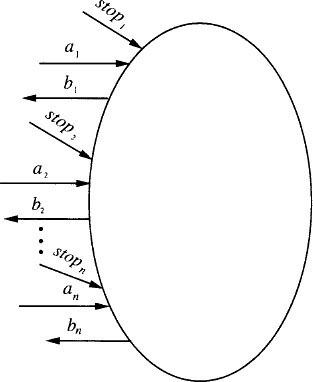
We begin by describing the external interface. We assume that A is accessed through n ports, numbered 1,…, n. Associated with each port i, A has some input actions of the form ai, where a is an invocation of the variable type, and some output actions of the form bi, where b is a response of the variable type. If ai is an input action, it means that a is an allowable invocation on port i, while if bi is an output action, it means that b is an allowable response on port i. We assume a technical condition: if ai is an input on port i and if f(a, v) = (b, w) for some v and w, then bi should be an output on port i. That is, if invocation a is allowed on port i, then all possible responses to a are also allowed on port i.
In addition, since we will consider the resiliency of atomic objects to stopping failures, we assume that there is an input stopi for each port i. The external interface is depicted in Figure 13.1.
Example 13.1.1 Read/write atomic object external interface
We describe an external interface for a 1-writer/2-reader atomic object for domain V. The object has three ports, which we label by 1, 2, and 3. Port 1 is a write port, supporting write operations only, while ports 2 and 3 are read ports, supporting read operations only. More precisely, associated with port 1 there are input actions of the form write(v)1 for all υ ∈ V and a single output action ack1. Associated with port 2 there is a single input action read2 and output actions of the form v2 for all υ ∈ V, and analogously for port 3. There are also stop1, stop2, and stop3 input actions, associated with ports 1, 2, and 3, respectively. The external interface is depicted in Figure 13.2.
Next, we describe the required behavior of an atomic object automaton A of a particular variable type ![]() . As in Chapters 10–12, we assume that A is composed with a collection of user automata Ui, one for each port. The outputs of Ui are assumed to be the invocations of A on port i, and the inputs of Ui are assumed to be the responses of A on port i. The stopi action is not part of the signature of Ui; it is assumed to be generated not by Ui, but by some unspecified external source.
. As in Chapters 10–12, we assume that A is composed with a collection of user automata Ui, one for each port. The outputs of Ui are assumed to be the invocations of A on port i, and the inputs of Ui are assumed to be the responses of A on port i. The stopi action is not part of the signature of Ui; it is assumed to be generated not by Ui, but by some unspecified external source.

The only other property we assume for Ui is that it preserve a “well-formedness” condition, defined as follows. Define a sequence of external actions of user Ui to be well-formed for user i provided that it consists of alternating invocations and responses, starting with an invocation. We assume that each Ui preserves well-formedness for i (according to the formal definition of “preserves” in Section 8.5.4). That is, we assume that the invocations of operations on each port are strictly sequential, each waiting for a response to the previous invocation. Note that this sequentiality requirement only refers to individual ports; we allow concurrency among the invocations on different ports.1 Throughout this chapter, we use the notation U to represent the composition of the separate user automata Ui, U = ΠUi.
We require that A ![]() U, the combined system consisting of A and U, satisfy several properties. First, there is a well-formedness condition similar to the ones used in Chapters 10, 11, and 12.
U, the combined system consisting of A and U, satisfy several properties. First, there is a well-formedness condition similar to the ones used in Chapters 10, 11, and 12.
Well-formedness: In any execution of A ![]() U and for any i, the interactions between Ui and A are well-formed for i.
U and for any i, the interactions between Ui and A are well-formed for i.
Since we have already assumed that the users preserve well-formedness, this amounts to saying that A also preserves well-formedness. This says that in the combined system A ![]() U, invocations and responses alternate on each port, starting with an invocation.
U, invocations and responses alternate on each port, starting with an invocation.
The next condition is the hardest one to understand. It describes the apparent atomicity of the operations, for a particular variable type T. Note that a trace of ![]() describes the correct responses to a sequence of invocations when all the operations are executed sequentially, that is, where each invocation after the first waits for a response to the previous invocation. The atomicity condition says that each trace produced by the combined system—which permits concurrent invocations of operations on different ports—“looks like” some trace of
describes the correct responses to a sequence of invocations when all the operations are executed sequentially, that is, where each invocation after the first waits for a response to the previous invocation. The atomicity condition says that each trace produced by the combined system—which permits concurrent invocations of operations on different ports—“looks like” some trace of ![]() .
.
The way of saying this formally is a little more complicated than you might expect, since we want a condition that makes sense even for executions of A ![]() U in which some of the invocations—the last ones on some ports—are incomplete, that is, have no responses. So we stipulate that each execution looks as if the operations that are completed and some of the incomplete ones are performed instantaneously at some points in their intervals.
U in which some of the invocations—the last ones on some ports—are incomplete, that is, have no responses. So we stipulate that each execution looks as if the operations that are completed and some of the incomplete ones are performed instantaneously at some points in their intervals.
In order to define atomicity for the system A ![]() U, we first give a more basic definition, of atomicity for a sequence of user actions. Namely, suppose that β is a (finite or infinite) sequence of external actions of A
U, we first give a more basic definition, of atomicity for a sequence of user actions. Namely, suppose that β is a (finite or infinite) sequence of external actions of A ![]() U that is well-formed
for every i (that is, for every i, β|ext(Ui) is well-formed for i). We say that β satisfies the atomicity property for
U that is well-formed
for every i (that is, for every i, β|ext(Ui) is well-formed for i). We say that β satisfies the atomicity property for ![]() provided that it is possible to do all of the following:
provided that it is possible to do all of the following:
- For each completed operation π, to insert a serialization point *π somewhere between π’s invocation and response in β.
- To select a subset Φ of the incomplete operations.
- For each operation π ∈ Φ, to select a response.
- For each operation π ∈ Φ, to insert a serialization point *π somewhere after π’s invocation in β.
These operations and responses should be selected, and these serialization points inserted, so that the sequence of invocations and responses constructed as follows is a trace of the underlying variable type ![]() :
:
For each completed operation π, move the invocation and response events appearing in β (in that order) to the serialization point *π. (That is, “shrink” the interval of operation π ∈ Φ to its serialization point.) Also, for each operation π, put the invocation appearing in β, followed by the selected response, at *π. Finally, remove all invocations of incomplete operations π ![]() Φ.
Φ.
Notice that the atomicity condition only depends on the invocation and response events—it does not mention the stop events. We can easily extend this definition to executions of A and of A ![]() U. Namely, suppose that α is any such execution that is well-formed for every i (that is, for every i, α|ext(Ui) is well-formed for i). Then we say that α satisfies the atomicity property for
U. Namely, suppose that α is any such execution that is well-formed for every i (that is, for every i, α|ext(Ui) is well-formed for i). Then we say that α satisfies the atomicity property for ![]() provided that its sequence of external actions, trace(α), satisfies the atomicity property for
provided that its sequence of external actions, trace(α), satisfies the atomicity property for ![]() .
.
Example 13.1.2 Executions with serialization points
Figure 13.3 illustrates some executions of a single-writer/single-reader read/write object with domain V = ![]() and initial value v0 = 0 that satisfy the atomicity property for the read/write register variable type. The serialization points are indicated by stars. Suppose that ports 1 and 2 are used for writing and reading, respectively.
and initial value v0 = 0 that satisfy the atomicity property for the read/write register variable type. The serialization points are indicated by stars. Suppose that ports 1 and 2 are used for writing and reading, respectively.
In (a), a read operation that returns 0 and a write(8) operation overlap and the serialization point for the read is placed before that of the write(8). Then if the operation intervals are shrunk to their serialization points, the sequence of invocations and responses is read2, 02, write(8)1, ack1. This is a trace of the variable type. (See Example 9.4.4.)
In (b), the same operation intervals are assigned serialization points in the opposite order. The resulting sequence of invocations and responses is then write(8)1, ack1, read2, 82, again a trace of the variable type.
Each of the executions in (c) and (d) includes an incomplete write(8) operation. In each case, a serialization point is assigned to the write(8), because its result is seen by a read operation. For (c), the result of shrinking the operation intervals is write(8)1, ack1, read2, 82, whereas for (d), the sequence is read2, 02, write(8)1, ack1, read2, 82. Both are traces of the variable type. (Again, see Example 9.4.4.)
In (e), there are infinitely many read operations that return 0, and consequently the incomplete write(8) cannot be assigned a serialization point.
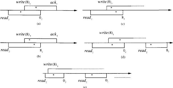
Figure 13.3: Executions of a single-writer/single-reader read/write object satisfying the atomicity property.
Example 13.1.3 Executions with no serialization points
Figure 13.4 illustrates some executions of a single-writer/single-reader read/write object that do not satisfy the atomicity property. In (a), there is no way to insert serialization points to explain the occurrence of a read that returns 8 followed by a read that returns 0. In (b), there is no way to explain the occurrence of a read that returns 0, after the completion of a write of 8.
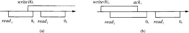
Figure 13.4: Executions of a single-writer/single-reader read/write object that do not satisfy the atomicity property.
Now we are (finally) ready to define the atomicity condition for the combined system A ![]() U.
U.
Atomicity: Let α be a (finite or infinite) execution of A ![]() U that is well-formed for every i. Then α satisfies the atomicity property (as defined just before Example 13.1.2).
U that is well-formed for every i. Then α satisfies the atomicity property (as defined just before Example 13.1.2).
We can also express the atomicity condition in terms of a trace property (see the definition of a trace property in Section 8.5.2). Namely, define the trace property P so that its signature sig(P) is the external interface of A ![]() U and its trace set traces(P) is exactly the set of sequences that satisfy both of the following:
U and its trace set traces(P) is exactly the set of sequences that satisfy both of the following:
- Well-formedness for every i
- The atomicity property for

(For convenience, we include the stop actions in the signature of P, even though they are not mentioned in the well-formedness and atomicity conditions.) The interesting thing about P is that it is a safety property, as defined in Section 8.5.3. That is, traces(P) is nonempty, prefix-closed, and limit-closed. This is not obvious, because the atomicity property has a rather complicated definition, involving the existence of appropriate placements of serialization points and selections of operations and responses.
Theorem 13.1 P (the trace property defined above, expressing the combination of well-formedness and atomicity) is a safety property.
The proof of Theorem 13.1 uses König’s Lemma, a basic combinatorial lemma about infinite trees:
Lemma 13.2 (König’s Lemma) If G is an infinite tree in which each node has only finitely many children, then G has an infinite path from the root.
Proof Sketch (of Theorem 13.1). Nonemptiness is clear, since λ ∈ traces(P).
For prefix-closure, suppose that β ∈ traces(P) and let β’ be a finite prefix of β. Since β ∈ traces(P), it is possible to select a set Φ of incomplete operations, a set of responses for the operations in Φ, and a set of serialization points that together demonstrate the correctness of β. We show how to make such selections for β’.
Let γ denote the sequence obtained from β by inserting the selected serialization points. Let γ’ be the prefix of γ ending with the last element of β’. Then γ’ includes serialization points for all the complete operations in β’ and some subset of the incomplete operations in β′. Choose Φ’, the set of incomplete operations for β′, to consist of those incomplete operations in β′ that have serialization points in γ’. Choose a response for each operation π ∈ Φ’ as follows: If π is incomplete in β, that is, if π ∈ Φ, then choose the same response that is chosen for π in β. Otherwise choose the response that actually appears in β. Then it is not hard to see that the chosen set Φ′, its chosen responses, and the serialization points in γ′ together demonstrate the correctness of β′. This shows prefix-closure.
Finally, we show limit-closure. Consider an infinite sequence β and suppose that all finite prefixes of β are in traces(P). We use König’s Lemma.
The tree G that we construct in order to apply König’s Lemma describes the possible placements of serialization points in β. Each node of G is labelled by a finite prefix of β, with serialization points inserted for some subset of the operations that are invoked in β. We only include labels that are “correct” in the sense that they satisfy the following three conditions:
- Every completed operation has exactly one serialization point, and that serialization point occurs between the operation’s invocation and response.
- Every incomplete operation has at most one serialization point, and that serialization point occurs after the operation’s invocation.
- Every response to an operation π is exactly the response that is calculated for π using the function of the given variable type at the serialization points. (Start with the initial value v0 and apply the function once for each serialization point, in order, with the corresponding invocation as the first argument. The response that is calculated for π is the response obtained when the function is applied for the serialization point *π.)
- The label of the root is λ.
- The label of each non-root node is an extension of the label of its parent.
- The label of each non-root node ends with an element of β.
- The label of each non-root node contains exactly one more element of β than does the label of its parent node (and possibly some more serialization points).
Thus, at each branch point in G, a decision is made about which serialization points to insert, in which order, between two particular symbols in β. By considering the prefix-closure construction above, we can see that G can be constructed so that every finite prefix β′ of β, with every “correct” assignment of serialization points prior to the last symbol of β′, appears as the label of some node of G.
Now we apply König’s Lemma to the tree G. First, it is easy to see that each node of G has only finitely many children. This is because only operations that have already been invoked can have their serialization points inserted and there are only finitely many places to insert these serialization points.
Second, we claim that G contains arbitrarily long paths from the root. This is because every finite prefix β′ of the infinite sequence β is in traces(P), which means that β′ has an appropriate assignment of serialization points. This assignment yields a corresponding path in G of length |β′|.
Since G contains arbitrarily long paths from the root, it is infinite. Then König’s Lemma (Lemma 13.2) implies that G contains an infinite path from the root. The node labels on this path yield a correct selection of serialization points (and consequently, of incomplete operations and responses) for the entire sequence β. ![]()
Having defined the safety properties for atomic objects—well-formedness and atomicity—we now turn to liveness properties. The liveness properties we consider are termination conditions similar to those we gave for the agreement problem, in Section 12.1. The simplest requirement is for failure-free executions, that is, those executions in which no stop event occurs.
Failure-free termination: In any fair failure-free execution of A ![]() U, every invocation has a response.
U, every invocation has a response.
With this one liveness property, we can define “atomic objects.” Namely, we say that A is an atomic object of variable type ![]() if it guarantees the well-formedness condition, the atomicity condition for
if it guarantees the well-formedness condition, the atomicity condition for ![]() , and the failure-free termination condition, for all collections of users.
, and the failure-free termination condition, for all collections of users.
Note that if we wanted to consider only the failure-free case, then we could simplify the statement of the atomicity condition, because there would never be any need to consider incomplete operations. The reason we have given the more complicated statement of the atomicity condition is that we shall also consider failures.
As for the mutual exclusion problem in Section 10.2, it is possible to reformulate the entire definition of an atomic object equivalently in terms of a trace property P. This time, sig(P) includes all the external interface actions of the atomic object, including the stop actions as well as the invocation and response actions, and traces(P) expresses well-formedness, atomicity, and failure-free termination. Then an automaton A with the right interface is an atomic object of type ![]() exactly if, for all collections of users, fairtraces(A
exactly if, for all collections of users, fairtraces(A ![]() U)
U) ![]() traces(P).
traces(P).
We also consider some stronger termination conditions involving fault-tolerance.
Wait-free termination: In any fair execution of A ![]() U, every invocation on a non-failing port has a response.
U, every invocation on a non-failing port has a response.
That is, any port on which no failure occurs provides responses for all invocations, regardless of the failures that occur on any of the other ports. We generalize this property to describe termination in the presence of any number of failures.
f-failure termination, 0 ≤ f ≤ n: In any fair execution of A ![]() U in which stop events occur on at most f ports, every invocation on a non-failing port has a response.
U in which stop events occur on at most f ports, every invocation on a non-failing port has a response.
Failure-free termination and wait-free termination are the special cases of the f-failure termination condition where f is equal to 0 and n, respectively. A further generalization allows us to talk about the failure of any particular set of ports.
I-failure termination, I ![]() {1,…, n}: In every fair execution of A
{1,…, n}: In every fair execution of A ![]() U in which the only stop events occur on ports in I, every invocation on a non-failing port has a response.
U in which the only stop events occur on ports in I, every invocation on a non-failing port has a response.
Thus, f-failure termination is the same as I-failure termination for all sets I of ports of size at most f. We say that A guarantees wait-free termination, guarantees I-failure termination, and so on, provided that it guarantees the corresponding condition for all collections of users.
We close this section with a simple example of a shared memory system that is an atomic object.
Example 13.1.4 A read/increment atomic object
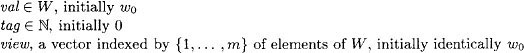
We define the read/increment variable type to have ![]() as its domain, 0 as its initial value, and read and increment as its operations.
as its domain, 0 as its initial value, and read and increment as its operations.
Let A be a shared memory system with n processes in which each port i supports both read and increment operations. A has n shared read/write registers x(i), 1 ≤ i ≤ n, each with domain ![]() and initial value 0. Shared variable x(i) is writable by process i and readable by all processes.
and initial value 0. Shared variable x(i) is writable by process i and readable by all processes.
When an incrementi input occurs on port i, process i simply increments its own shared variable, x(i). It can do this using only a write operation, by remembering the value of x(i) in its local state. When a readi occurs on port i, process i reads all the shared variables x(j) one at a time, in any order, and returns the sum.
Then it is not hard to see that A is a read/increment atomic object and that it guarantees wait-free termination. For example, to see the atomicity condition, consider any execution of A ![]() U. Let Φ be the set of incomplete increment operations for which a write occurs on a shared variable. For each increment operation π that is either completed or is in Φ, place the serialization point *π at the point of the write.
U. Let Φ be the set of incomplete increment operations for which a write occurs on a shared variable. For each increment operation π that is either completed or is in Φ, place the serialization point *π at the point of the write.
Now, note that any completed (high-level) read operation π returns a value v that is no less than the sum of all the x(i)’s when the read is invoked and no greater than the sum of all the x(i)’s when the read completes. Since each increment operation only increases this sum by 1, there must be some point within π’s interval at which the sum of the x(i)’s is exactly equal to the return value v. We place the serialization point *π at this point. These choices allow the shrinking needed to show atomicity.
13.1.2 A Canonical Wait-Free Atomic Object Automaton
In this subsection we give an example of an atomic object automaton C for a given variable type ![]() and given external interface. Automaton C guarantees wait-free termination. C is highly nondeterministic and is sometimes regarded as a “canonical wait-free atomic object automaton” for the given type and external interface. It can be used to help show that other automata are wait-free atomic objects.
and given external interface. Automaton C guarantees wait-free termination. C is highly nondeterministic and is sometimes regarded as a “canonical wait-free atomic object automaton” for the given type and external interface. It can be used to help show that other automata are wait-free atomic objects.
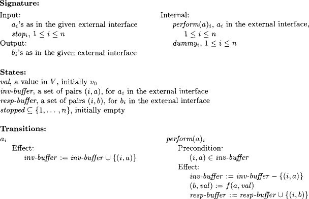
C automaton (informal):
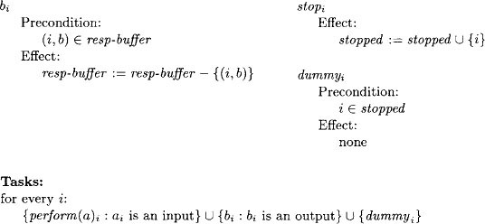
C maintains an internal copy of a shared variable of type ![]() , initialized to the initial value v0. It also has two buffers, inv-buffer for pending invocations and resp-buffer for pending responses, both initially empty.
, initialized to the initial value v0. It also has two buffers, inv-buffer for pending invocations and resp-buffer for pending responses, both initially empty.
Finally, it keeps track of the ports on which a stop action has occurred, in a set stopped, initially empty.
When an invocation arrives, C simply records it in inv-buffer. At any time, C can remove any pending invocation from inv-buffer and perform the requested operation on the internal copy of the shared variable. When it does this, it puts the resulting response in resp-buffer. Also at any time, C can remove any pending response from resp-buffer and convey the response to the user.
A stopi event just adds i to stopped, which enables a special dummyi action having no effect. It does not, however, disable the other locally controlled actions involving i. All the locally controlled actions involving each port i, including the dummyi action, are grouped into one task. This means that after a stopi, actions involving i are permitted (but not required) to cease.
More precisely,
C automaton (formal):
Theorem 13.3 C is an atomic object with the given type and external interface, guaranteeing wait-free termination (for all collections of users).
Proof Sketch. Well-formedness is straightforward. To see wait-freedom, consider any fair execution α of C ![]() U and suppose that there are no failures on port i in α. Then the dummyi action is never enabled in α. The fairness of α then implies that every invocation on port i triggers a performi event and a subsequent response.
U and suppose that there are no failures on port i in α. Then the dummyi action is never enabled in α. The fairness of α then implies that every invocation on port i triggers a performi event and a subsequent response.
It remains to show atomicity. Consider any execution α of C ![]() U. Let Φ be the set of incomplete operations for which a perform occurs in α. Assign a serialization point *π to each operation π that is either completed in α or is in Φ: place *π at the point of the perform. Also, for each π ∈ Φ, select the response returned by the perform as the response for the operation. These choices allow the shrinking needed to show atomicity.
U. Let Φ be the set of incomplete operations for which a perform occurs in α. Assign a serialization point *π to each operation π that is either completed in α or is in Φ: place *π at the point of the perform. Also, for each π ∈ Φ, select the response returned by the perform as the response for the operation. These choices allow the shrinking needed to show atomicity. ![]()
C can be used to help verify that other automata are also wait-free atomic objects, as follows:
Theorem 13.4 Suppose that A is an I/O automaton with the same external interface as C. Suppose that fairtraces(A ![]() U)
U) ![]() fairtraces(C
fairtraces(C ![]() U) for every composition U of user automata. Then A is an atomic object guaranteeing wait-free termination.
U) for every composition U of user automata. Then A is an atomic object guaranteeing wait-free termination.
Proof Sketch. Follows from Theorem 13.3. For the well-formedness and atomicity, we use the fact that the combination of these two conditions is a safety property (Theorem 13.1), plus the fact that every finite trace can be extended to a fair trace (Theorem 8.7). The wait-freedom condition follows immediately from the definitions.
We also have a converse to Theorem 13.4, which says that every fair trace that is allowed for a wait-free atomic object is actually generated by C:
Theorem 13.5 Suppose that A is an I/O automaton with the same external interface as C. Suppose that A is an atomic object guaranteeing wait-free termination. Then fairtraces(A ![]() U)
U) ![]() fairtraces(C
fairtraces(C ![]() U), for every composition U of user automata.
U), for every composition U of user automata.
Proof. The proof is left as an exercise.
13.1.3 Composition of Atomic Objects
In this subsection, we give a theorem that says that the composition of atomic objects (using ordinary I/O automaton composition, defined in Section 8.2.1) is also an atomic object. Recall the definitions of compatible variable types and composition of variable types from the end of Section 9.4.
Theorem 13.6 Let {Aj}j∈J be a countable collection of atomic objects having compatible variable types {Tj}j∈J and all having the same set of ports {1,…, n}. Then the composition A = ∏ j∈J is an atomic object having variable type T = ∏j∈J Tj and having ports {1,…, n}.
Furthermore, if every Aj guarantees I-failure termination (for all collections of users), then so does A.
In atomic object A, port i handles all the invocations and responses that are handled on port i of any of the Aj. According to the definition of composition, the state of A has a piece for each Aj. The invocations and responses that are derived from Aj only involve the piece of the state of A associated with Aj. The stopi actions, however, affect all parts of the state. We leave the proof of Theorem 13.6 for an exercise.
13.1.4 Atomic Objects versus Shared Variables
The definition of an atomic object says that its traces “look like” traces of a sequentially accessed shared variable of the underlying type. What good is this?
The most important fact about atomic objects, from the point of view of system construction, is that it is possible to substitute them for shared variables in a shared memory system. This permits modular construction of systems: it is possible first to design a shared memory system and then to replace the shared variables by arbitrary atomic objects of the given types. Under certain circumstances, the resulting system “behaves in the same way” as the original shared memory system, as far as the users can tell.
In this section, we describe this substitution technique. First we give some technical conditions on the original shared memory system that are required for the replacement to work correctly. Next, we give the substitution construction. Finally, we define the sense in which the resulting system behaves in the same way as the original system and prove that, with the given conditions, the resulting system really does behave in the same way. Although the basic ideas are reasonably simple, there are a few details that have to be handled carefully in order to make the substitution technique work out right.
We begin with A, an arbitrary algorithm in the shared memory model of Chapter 9. We assume that A interacts with user automata Ui, 1 ≤ i ≤ n. We permit each process i of A to have any number of tasks. We also include stopi actions, as discussed in Section 9.6, and assume that each stopi event permanently disables all the tasks of process i.
Now for the technical conditions we mentioned above. Consider A in combination with any collection of user automata Ui. We assume that for each port i, there is a function turni that, for any finite execution α of the combined system, yields either the value system or user. This is supposed to indicate whose turn it is to take the next step, after α. Specifically, we require that if turni(α) = system, then Ui has no output step enabled in its state after α, while if turni(α) = user, then process i of A has no output or internal step, that is, no locally controlled step, enabled in its state after α.
For example, all the mutual exclusion algorithms in Chapter 10 and all the resource-allocation algorithms in Chapter 11 satisfy these conditions (if we add the stop actions). In those cases, turni(α) = system for any α after which Ui is in the trying or exit region, and turni(α) = user if Ui is in the critical or remainder region. In fact, the required conditions are implied by the restriction on process activity assumed near the end of Section 10.2 and at the end of Section 11.1.2.
For consensus algorithms, as studied in Chapter 12, we may define turni(α) = system for any α that contains an initi event, and turni(α) = user otherwise. Then to satisfy the conditions we need here, we would have to add a restriction, namely, that process i cannot do anything before an initi occurs. This condition is satisfied by the only algorithm in Chapter 12, RMWAgreement.
Now we give the substitution. Suppose that for each shared variable x of A, we are given an atomic object automaton Bx of the same type and the appropriate external interface. That is, Bx has ports 1,…, n, one for each process of A. On each port, it allows all invocations and responses that are used by process i in its interactions with shared variable x in algorithm A. It also has stopi inputs, one for each port, as usual.
Then we define Trans(A), the transformed version of A that uses the atomic objects Bx in place of its shared variables, to be the following automaton:
Trans(A) automaton:
Trans(A) is a composition of I/O automata, one for each process i and one for each shared variable x of algorithm A. For each variable x, the automaton is the atomic object automaton Bx. For each process i, the automaton is Pi, defined as follows.
The inputs of Pi are the inputs of A on port i plus the responses of each Bx on port i plus the stopi action. The outputs of Pi are the outputs of A on port i plus the invocations for each Bx on port i.
Pi’s steps simulate those of process i of A directly, with the following exceptions: When process i of A performs an access to shared variable x, Pi instead issues the appropriate invocation to Bx. After it does this, it suspends its activity, awaiting a response by Bx to the invocation. When a response arrives, Pi resumes simulating process i of A as usual. There is a task of Pi corresponding to each task of process i of A.
If a stopi event occurs, all tasks of Pi are thereafter disabled.
Example 13.1.5 A and Trans(A)
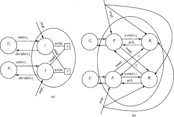
Consider a two-process shared memory system A that is supposed to solve some sort of consensus problem, using two read/write shared variables, x and y. We assume that process 1 writes x and reads y, and process 2 writes y and reads x. The interface between each Ui and A consists of actions of the form init(v)i, which are outputs of Ui and inputs of A, and actions of the form decide(v)i, which are outputs of A and inputs of Ui. In addition, stopi, i ∈ {1, 2} is an input of A. The architecture of this system is depicted in Figure 13.5, part (a).
The architecture of the transformed system Trans(A) is depicted in part (b). Note the external interfaces of the automata Bx and By. For example, Bx has inputs write(v)1 and read2 and outputs ack1 and v2.2 Bx also has inputs stop1 and stop2, which are identified with the stop1 input to P1 and the stop2 input to P2, respectively. This means, for example, that stop1 simultaneously disables all tasks of P1 and also has whatever effect stop1 has on the implementation Bx.
Now we give a theorem describing what is preserved by transformation Trans. Theorem 13.7 first describes conditions that hold for any execution α of Trans(A). Execution α does not have to be fair for these conditions to hold. These conditions say that α looks to the users like an execution α′ of A. Moreover, the same stop events occur in α and α′, although we allow for the possibility that the stop events could occur in different positions in the two executions.
Theorem 13.7 then goes on to identify some conditions under which the simulated execution α′ of the A system is guaranteed to be a fair execution. As you would expect, one of the conditions is that α is itself a fair execution of the Trans(A) system. But this is not enough—we also need to make sure that the object automata Bx do not cause processing to stop. So we include two other conditions that together ensure that this does not happen, namely, that all the failures that occur in α are confined to a particular set I of ports and that all the object automata Bx can tolerate failures on I (formally, they guarantee I-failure termination).
Theorem 13.7 Suppose that α is any execution of the system Trans(A) ![]() U. Then there is an execution α′ of A
U. Then there is an execution α′ of A ![]() U such that the following conditions hold:
U such that the following conditions hold:
- α and α′ are indistinguishable3 to U.
- For each i, a stopi occurs in α exactly if a stopi occurs in α′.
Moreover, if α is a fair execution, if every i for which stopi appears in α is in I, and if every Bx guarantees I-failure termination (for all collections of users), then α′ is also a fair execution.
Proof Sketch. We modify α to get α′ as follows. First, since each Bx is an atomic object, we can insert a serialization point *π in α between the invocation and response of each completed operation π on Bx and also after the invocation of each of a subset Φ of the incomplete operations on Bx. We also obtain responses for all the operations in Φ. These serialization points and responses can be guaranteed to satisfy the “shrinking” property described in the atomicity condition.
Next, we move the invocation and response events for each completed operation π on Bx so that they are adjacent and occur exactly at *π. Also, for each incomplete operation π in Φ—that is, each incomplete operation that has been assigned a serialization point—we place the invocation, together with the newly manufactured response, at *π. And for each incomplete operation that is not in Φ—that is, each incomplete operation that has not been assigned a serialization point—we simply remove the invocation event. There is one additional technicality: if any stopi event in α occurs after an invocation by process i and before the serialization point to which the invocation is moved, then that stopi event is also moved to the serialization point, just after the invocation and response. We move, add, and remove events in this way for all shared variables x.
We claim that it is possible to move all the events that we have moved in this construction without changing the order of events of any Pi (with one technical exception: a response to Pi by some Bx may be moved ahead of a stopi). This follows from two facts. First, by construction, Pi performs no locally controlled actions while it is waiting for a response to an invocation. And second, while Pi is waiting for a response, it is the system’s turn to take steps. This means that Ui will not perform any output steps, so Pi will receive no inputs.
Similarly, we claim that we can add the responses we have added and remove the invocations we have removed in this construction without otherwise affecting the behavior of Pi. This is because if Pi performs an incomplete operation in α, it does not do anything after that operation. It does not matter if Pi stops just before issuing the invocation, while waiting for a response, or just after receiving the response.
Since we have not changed anything significant by this motion, addition, and removal of events, we can simply fill in the states of the processes Pi as in α. (A technical exception: A response to Pi moved before a stopi might cause a different change in the state of Pi than it did in α.) The result is a new execution, α1, also of the system Trans(A) ![]() U. Moreover, it is clear that α and α1 are indistinguishable to U and have stop events for the same ports.
U. Moreover, it is clear that α and α1 are indistinguishable to U and have stop events for the same ports.
Now, α1 is an execution of Trans(A) ![]() U, which is not exactly what we need; rather, we need an execution of the system A
U, which is not exactly what we need; rather, we need an execution of the system A ![]() U. But notice that in α1, all the invocations and responses for the object automata Bx occur in consecutive matching pairs. So we replace those pairs by instantaneous accesses to the corresponding shared variables and thereby obtain an execution α′ of the system A
U. But notice that in α1, all the invocations and responses for the object automata Bx occur in consecutive matching pairs. So we replace those pairs by instantaneous accesses to the corresponding shared variables and thereby obtain an execution α′ of the system A ![]() U. Then α and α′ are indistinguishable to U and have stop events for the same ports. This proves the first half of the theorem.
U. Then α and α′ are indistinguishable to U and have stop events for the same ports. This proves the first half of the theorem.
For the second half, suppose that α is a fair execution of Trans(A) ![]() U, that I
U, that I ![]() {1,…, n}, that every i for which stopi appears in α is in I, and that each Bx guarantees I-failure termination. Then the only stopi inputs received by any Bx must be for ports i ∈ I. Thus, since every Bx guarantees I-failure termination, it must be that every Bx provides responses for every invocation by a process Pi for which no stopi event occurs in α. This fact, combined with the fairness assumption for processes Pi, is enough to imply that α′ is a fair execution of A
{1,…, n}, that every i for which stopi appears in α is in I, and that each Bx guarantees I-failure termination. Then the only stopi inputs received by any Bx must be for ports i ∈ I. Thus, since every Bx guarantees I-failure termination, it must be that every Bx provides responses for every invocation by a process Pi for which no stopi event occurs in α. This fact, combined with the fairness assumption for processes Pi, is enough to imply that α′ is a fair execution of A ![]() U.
U.
Thus, Theorem 13.7 implies that any algorithm for the shared memory model (with some simple restrictions) can be transformed to work with atomic objects instead of shared variables and that the users cannot tell the difference.
We give as a corollary the special case of Theorem 13.7 where the atomic objects Bx all guarantee wait-free termination. In this case, we can conclude that α′ is fair just by assuming that α is fair.
Corollary 13.8 Suppose that all the Bx guarantee wait-free termination. Suppose that α is any fair execution of Trans(A) x U. Then there is a fair execution α′ of A x U such that the following conditions hold:
- α and α′ are indistinguishable to U.
- For each i, a stopi occurs in α exactly if a stopi occurs in α′.
Proof. Immediate from Theorem 13.7, letting I = {1,…, n}.
In the special case where A is itself an atomic object, Theorem 13.7 implies that Trans(A) is also an atomic object. Including failure considerations, we obtain the following corollary.
Corollary 13.9 Suppose that A and all the Bx’s are atomic objects guaranteeing I-failure termination. Then Trans(A) is also an atomic object guaranteeing I-failure termination.
Proof. First let α be any execution of Trans(A) and a collection of users Ui. Then Theorem 13.7 yields an execution α′ of A ![]() U such that α and α′ are indistinguishable to U. Since A is an atomic object, α′ satisfies the well-formedness and atomicity properties. Since both of these are properties of the external interface of U, and α and α′ are indistinguishable to U, α also satisfies the well-formedness and atomicity properties.
U such that α and α′ are indistinguishable to U. Since A is an atomic object, α′ satisfies the well-formedness and atomicity properties. Since both of these are properties of the external interface of U, and α and α′ are indistinguishable to U, α also satisfies the well-formedness and atomicity properties.
It remains to consider the I-failure termination condition. Let α be any fair execution of Trans(A) and a collection of users Ui such that every i for which stopi appears in α is in I. Since all the Bx guarantee I-failure termination, Theorem 13.7 yields a fair execution α′ of A ![]() U, such that α and α′ are indistinguishable to U and α and α′ contain stop events for the same set of ports. Thus, every i for which stopi appears in α′ is in I.
U, such that α and α′ are indistinguishable to U and α and α′ contain stop events for the same set of ports. Thus, every i for which stopi appears in α′ is in I.
Now consider any invocation in α on a port i for which no stopi event occurs in α—that is, on a non-failing port. Since α and α′ are indistinguishable to U, the same invocation appears in α′. Because A guarantees I-failure termination, there is a corresponding response event in α′. Then, since α and α′ are indistinguishable to U, this response also appears in α. This is enough to show I-failure termination.
Hierarchical construction of shared memory systems. In the special case where each atomic object Bx is itself a shared memory system, we claim that Trans(A) can also be viewed as a shared memory system. Namely, each process i of Trans(A) (viewed as a shared memory system) is a combination of process Pi of Trans(A) and the processes indexed by i in all of the shared memory systems Bx. This combination is not exactly an I/O automaton composition, because the processes in the Bx’s are not I/O automata. However, the combination is easy to describe: the state set of process i of Trans(A) is just the Cartesian product of the state set of Pi and the state sets of all the processes indexed by i in all the Bx’s, and likewise for the start states. The actions associated with process i of Trans(A) are just the actions of all the component processes i, and similarly for the tasks.
The situation is depicted in Figure 13.6. Part (a) shows Trans(A), including the shared memory systems Bx plugged in for all the shared variables x of A. (For simplicity, we have not drawn the stop input arrows.) All the shaded processes are associated with port 1. Part (b) shows the same system as in part (a), with the processes that are to be combined grouped together. Thus, all the shaded processes from part (a) are now combined into a single process 1 in part (b).
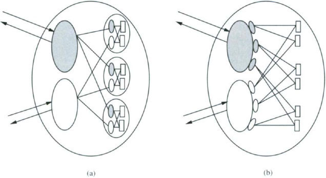
By the definition of Trans(A), the effect of a stopi event in the system of part (a) is to immediately stop all tasks of all the processes associated with port i—the tasks of Pi as well as the tasks of all the processes i of the Bx’s. This is the same as saying that stopi stops all tasks of the composed process i in the system of part (b), which is just what stopi is supposed to do when that system is regarded as a shared memory system.
Hierarchical construction of atomic objects. Finally, consider the very special case where shared memory system A is an atomic object guaranteeing I-failure termination and each atomic object Bx is a shared memory system that guarantees I-failure termination. Then Corollary 13.9 and the previous paragraph imply that Trans(A) is an atomic object guaranteeing I-failure termination and also that it is a shared memory system. This observation says that two successive layers of atomic object implementations in the shared memory model can be collapsed into one.
13.1.5 A Sufficient Condition for Showing Atomicity
Before presenting specific atomic object constructions, we give a sufficient condition for showing that a shared memory system guarantees the atomicity condition. This lemma enables us to avoid reasoning explicitly about incomplete operations in many of our proofs that objects are atomic.
For this lemma, we suppose that A is a shared memory system with an external interface appropriate for an atomic object for variable type ![]() . Also, we suppose that Ui, 1 ≤ i ≤ n, is any collection of users for A; as usual, U = Π Ui.
. Also, we suppose that Ui, 1 ≤ i ≤ n, is any collection of users for A; as usual, U = Π Ui.
Lemma 13.10 Suppose that the combined system A x U guarantees well-formedness and failure-free termination. Suppose that every (finite or infinite) execution α of A x U containing no incomplete operations satisfies the atomicity property. Then the same is true for every execution of A x U, including those with incomplete operations.
Proof. Let α be an arbitrary finite or infinite execution of the combined system A x U, possibly containing incomplete operations. We must show that α satisfies the atomicity property, that is, that α|ext(U) satisfies the atomicity property.
If α is finite, then the handling of stop events in a shared memory system implies that there is a finite failure-free execution α1, obtained by removing the stop events from α (and possibly modifying some state changes associated with inputs at ports on which a stop has occurred), such that α1|ext(U) = α|ext(U). By basic properties of I/O automata (in particular, Theorem 8.7), α1 can be extended to a fair failure-free execution α2 of A x U. Since A guarantees failure-free termination, every operation in α2 is completed. Then, by assumption, α2 satisfies the atomicity property, that is, α2|ext(U) satisfies the atomicity property. But α1|ext(U) is a prefix of α2|ext(U). Since, by Theorem 13.1, atomicity combined with well-formedness is a safety property and hence is prefix-closed, it follows that α1|ext(U) satisfies the atomicity property. Since α|ext(U) = α1|ext(U), we have that α|ext(U) satisfies the atomicity property, as needed.
On the other hand, suppose that α is infinite. By what we have just proved, any finite prefix α1 of α has the property that α1|ext(U) satisfies the atomicity property. But α|ext(U) is just the limit of the sequences of the form α1|ext(U). Since, by Theorem 13.1, atomicity combined with well-formedness is a safety property and hence is limit-closed, it follows that α|ext(U) satisfies the atomicity property, as needed.
13.2 Implementing Read-Modify-Write Atomic Objects in Terms of Read/Write Variables
We consider the problem of implementing a read-modify-write atomic object in the shared memory model with read/write shared variables. (See Section 9.4 for the definition of a read-modify-write variable type.) To be specific, we fix an arbitrary n and suppose that the read-modify-write object being implemented has n ports, each of which can support arbitrary update functions as inputs.
If all we require is an atomic object and we are not concerned about tolerating failures, then there are simple solutions. For instance,
RMWfromRW algorithm:
The latest value of the read-modify-write variable corresponding to the object being implemented is kept in a read/write shared variable x. Using a set of read/write shared variables different from x, the processes perform the trying part of a lockout-free mutual exclusion algorithm (for example, PetersonNP from Section 10.5.2) whenever they want to perform operations on the atomic object. When a process i enters the critical region of the mutual exclusion algorithm, it obtains exclusive access to x. Then process i performs its read-modify-write operation using a read step followed by a separate write step. After completing these steps, process i performs the exit part of the mutual exclusion algorithm.
However, this algorithm is not fault-tolerant: a process might fail while it is in its critical region, thereby preventing any other process from accessing the simulated read-modify-write variable. In fact, this limitation is not an accident. We give an impossibility result, even for the case where only a single failure is to be tolerated.
Theorem 13.11 There does not exist a shared memory system using read/write shared variables that implements a read-modify-write atomic object and guarantees 1-failure termination.
Proof. Suppose for the sake of contradiction that there is such a system, say B. Let A be the RMWAgreement algorithm for agreement in the read-modify-write shared memory model, given in Section 12.3. By Theorem 12.9, A guarantees wait-free termination and hence guarantees 1-failure termination (as defined for agreement algorithms in Section 12.1). Now we apply the transformation of Section 13.1.4 to A, using B in place of the single shared read-modify-write variable of A. Let Trans(A) denote the resulting system.
Claim 13.12 Trans(A) solves the agreement problem of Chapter 12 and guarantees 1-failure termination.
Proof. The proof of this is similar to that of Corollary 13.9. First let α be any execution of Trans(A) and a collection of users Ui. Then Theorem 13.7 yields an execution α′ of A x U such that α and α′ are indistinguishable to U. Since A solves the agreement problem, α′ satisfies the well-formedness, agreement, and validity properties. Then since α and α′ are indistinguishable to U, α also satisfies the well-formedness, agreement, and validity properties.
It remains to consider the 1-failure termination condition. Let α be any fair execution of Trans(A) and a collection of users Ui, in which init events occur on all ports and in which there is a stop event for at most one port. Since B guarantees 1-failure termination, Theorem 13.7 yields a fair execution α′ of A x U such that α and α′ are indistinguishable to U and contain stop events for the same set of ports. Thus, init events occur on all ports in α′, and there is a stop event for at most one port in α′.
Now consider any port i with no stopi event in α. Since α and α′ contain stop events for the same ports, there is also no stopi event in α′. Because A guarantees 1-failure termination, there is a decidei event in α′. Then, since α and α′ are indistinguishable to U, this decidei also appears in α. This is enough to show 1-failure termination.
However, by the paragraph at the end of Section 13.1, Trans(A) is itself a shared memory system in the read/write shared memory model. But then Trans(A) contradicts Theorem 12.8, the impossibility of agreement with 1-failure termination in the read/write shared memory model.
13.3 Atomic Snapshots of Shared Memory
In the rest of this chapter, we consider the implementation of particular types of atomic objects in terms of other types of atomic objects, or, equivalently, in terms of shared variables. This section is devoted to snapshot atomic objects, and the next is devoted to read/write atomic objects.
In the read/write shared memory model, it would be useful for a process to be able to take an instantaneous snapshot of the entire state of shared memory. Of course, the read/write model does not directly provide this capability—it only permits reads on individual shared variables.
In this section, we consider the implementation of such a snapshot. We formulate the problem as that of implementing a particular type of atomic object called a snaphot atomic object, using the read/write shared memory model. The variable type underlying a snapshot atomic object has as its domain V the set of vectors of some fixed length over a more basic domain W. The operations are of two kinds: writes to individual vector components, which we call update operations, and reads of the entire vector, which we call snap operations. A snapshot atomic object can simplify the task of programming a read/write system by allowing the processes to view the entire shared memory as a vector accessible by these powerful operations.
We start with a description of the problem, then give a simple solution that uses read/write shared variables of unbounded size. Then we show how the construction can be modified to work with bounded-size shared variables. Section 13.4.5 contains an application of snapshot atomic objects in the implementation of read/write atomic objects.
13.3.1 The Problem
We first define the variable type ![]() to which the snapshot atomic object will correspond; we call this a snapshot variable type.
to which the snapshot atomic object will correspond; we call this a snapshot variable type.
The definition begins with an underlying domain W with initial value ω0. The domain V of ![]() is then the set of vectors of elements of ω of a fixed length m. The initial value v0 is the vector in which every component has the value ω0. There are invocations of the form update(i, w), where 1 ≤ i ≤ m and ω∈ W, with response ack, and an invocation snap, with responses v ∈ V. An update(i, ω) invocation causes component i of the current vector to be set to the value ω and triggers an ack response. A snap invocation causes no change to the vector but triggers a response containing the current value of the entire vector.
is then the set of vectors of elements of ω of a fixed length m. The initial value v0 is the vector in which every component has the value ω0. There are invocations of the form update(i, w), where 1 ≤ i ≤ m and ω∈ W, with response ack, and an invocation snap, with responses v ∈ V. An update(i, ω) invocation causes component i of the current vector to be set to the value ω and triggers an ack response. A snap invocation causes no change to the vector but triggers a response containing the current value of the entire vector.
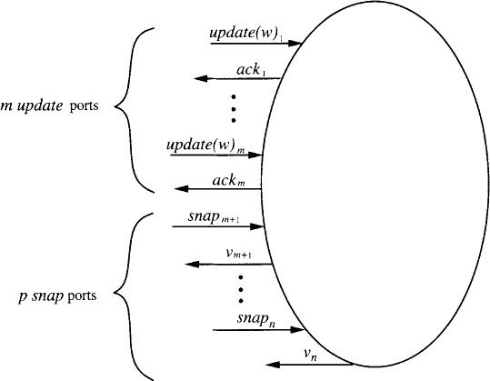
Next we define the external interface that we will consider. We assume that there are exactly n = m + p ports, where m is the fixed length of the vectors and p is some arbitrary positive integer. The first m ports are the update ports, and the remaining p ports are the snap ports. On each port i, 1 ≤ i ≤ m, we permit only invocations of the form update(i, w)—that is, only updates to the ith vector component are handled on port i. We sometimes abbreviate the redundant notation update(i, w)i, which indicates an invocation of update(i, w) on port i, as simply update(ω)i. On each port i, m + 1 ≤ i ≤ n, we permit only snap invocations. See Figure 13.7.
Notice that we are considering a special case of the general problem, where updates to each vector component arrive only at a single designated port and hence arrive sequentially. It is also possible to consider a more general case, where many ports allow updates to the same vector component. Of course, we could also consider the case where update and snap operations are allowed to occur on the same port.
We consider implementing the atomic object corresponding to this variable type and external interface using a shared memory system with n processes, one per port. We assume that all the shared variables are 1-writer/n-reader read/write shared variables. The implementations we describe guarantee wait-free termination.
13.3.2 An Algorithm with Unbounded Variables
The UnboundedSnapshot algorithm uses m 1-writer/n-reader read/write shared variables x(i), 1 ≤ i ≤ m. Each variable x(i) can be written by process i (the one connected to port i, which is the port for update(i, w) operations) and can be read by all processes. The architecture appears in Figure 13.8. Each variable x(i) holds values each of which consists of an element of ω plus some additional values needed by the algorithm. One of these additional values is an unbounded integer “tag.”

In the UnboundedSnapshot algorithm, each process i writes the values that it receives in updatei invocations into the shared variable x(i). A process performing a snap operation must somehow obtain consistent values from all the shared variables, that is, values that appear to have coexisted in the shared memory at some moment in time. The way it does this is based on two simple observations.
Observation 1: Suppose that whenever a process i performs an update(ω)i operation, it writes not only the value ω into x(i), but also a “tag” that uniquely identifies the update. Then, if a process j that is attempting to perform a snap operation reads all the shared variables twice, with the second set of reads starting after the first set of reads is finished, and if it finds the tag in each variable x(i) to be the same in the first and second set of reads, then the common vector of values returned in the two sets of reads is in fact a vector that appears in shared memory at some point during the interval of the snap operation. In particular, this vector is the vector of values at any point after the completion of the first set of reads and before the start of the second set.
Observation 1 suggests the following simple algorithm. Each process i performing an update(ω) operation writes ω into x(i), along with a unique local tag, obtained by starting with 1 for the first update at i and incrementing for each successive update at i.
Each process j performing a snap repeatedly performs a set of reads, one per shared variable, until two consecutive sets of reads are “consistent,” that is, they return identical tags for every x(i). When this happens, the vector of values returned by the second set of reads (which must be the same as that returned by the first set of reads) is returned as the response to the snap operation.
It is easy to see that whenever this simple algorithm completes an operation, the response is always “correct,” that is, it satisfies the well-formedness and atomicity conditions. However, it fails to guarantee even failure-free termination: a snap may never return, even in the absence of process failures, if new update operations keep getting invoked while the snap is active. A way out of this difficulty is provided by
Observation 2: If process j, while performing repeated sets of reads on behalf of a snap, ever sees the same variable x(i) with four different tags—say tag1, tag2, tag3, and tag4—then it knows that some updatei operation is completely contained within the interval of the current snap. In particular, the updatei operation that writes tag3 must be totally contained within the current snap.
To see why this is so, we argue first that the update that writes tag3 must begin after the beginning of the snap. This is because it begins after the end of the update that writes tag2, and the end of the update that writes tag2 must happen after the beginning of the snap interval (since the snap sees tag1).
Second, we argue that the update that writes tag3 must end before the end of the snap. This is because it ends before the beginning of the update that writes tag4, and the snap sees tag4.
Observations 1 and 2 suggest the UnboundedSnapshot algorithm. It extends the simple algorithm above so that before an update process i writes to x(i), it first executes its own embedded-snap subroutine, which is just like a snap. Then, when it writes its value and tag in x(i), it also places the result of its embedded-snap in x(i). A snap that fails to discover two sets of reads with identical tags despite many repeated attempts can use the result of an embedded-snap as a default snapshot value. A more careful description follows. In this description, each shared variable is a record with several fields; we use dot notation to indicate the fields.
UnboundedSnapshot algorithm:
Each shared variable x(i), 1 ≤ i ≤ m, is writable by process i and readable by all processes. It contains the following fields:
When a snapj input occurs on port j, m + 1 ≤ j ≤ n, process j behaves as follows. It repeatedly performs sets of reads, where a set consists of m reads, one read of each shared variable x(i), 1 ≤ i ≤ m, in any order. It does this until one of the following happens:
- Two sets of reads return the same x(i).tag for every i.
In this case, the snap returns the vector of values x(i).val, 1 ≤ i ≤ m, returned by the second set of reads. (This is the same as the vector returned by the first set of reads.)
- For some i, four distinct values of x(i).tag have been seen.
In this case, the snap returns the vector of values in x(i).view associated with the third of the four values of x(i).tag.
When an update(ω)i input occurs, process i behaves as follows. First, it performs an embedded-snap. This involves exactly the same work as is performed by a snap, except that the vector determined is recorded locally by process i instead of being returned to the user. Second, process i performs a single write to x(i), setting the three fields of x(i) as follows:
- x(i).val := ω
- x(i).tag is set to the smallest unused tag at i.
- x(i).view is set to the vector returned by the embedded-snap.
Finally, process i outputs acki.
Theorem 13.13 The UnboundedSnapshot algorithm is a snapshot atomic object guaranteeing wait-free termination.
Proof. The well-formedness condition is clear. Wait-free termination is also easy to see: the key is that every snap and every embedded-snap must terminate after performing at most 3m + 1 sets of reads. This is because after 3m + 1 sets of reads, there must either be two consecutive sets with no changes or else some variable x(i) with at least four different tags. In either of these two cases, the operation terminates.
It remains to show the atomicity condition. Fix any execution α of the UnboundedSnapshot algorithm plus users. In view of Lemma 13.10, we may assume without loss of generality that α contains no incomplete operations. We describe how to insert serialization points for all operations.
We insert the serialization point for each update operation at the point at which its write occurs. The insertion of serialization points for snap operations is a little more complicated. To describe this insertion, we find it helpful to assign serialization points not just to the snap operations but also to the embedded-snap operations.
First, consider any snap or embedded-snap that terminates by finding two consistent sets of reads. For each such operation, we insert the serialization point anywhere between the end of the first of its two sets of reads and the beginning of its second.
Second, consider those snap and embedded-snap operations that terminate by finding four different tags in the same variable. We insert serialization points for these operations one by one, in the order of their response events. For each such operation π, note that the vector it returns is the result of an embedded-snap ϕ whose interval is totally contained within the interval of operation π. Note that this operation ϕ has already been assigned a serialization point, since it completes earlier than π. We insert the serialization point for π at the same place as that for ϕ.
It is easy to see that all the serialization points are within the required intervals. For the update operations and for the snap and embedded-snap operations that terminate by finding two consistent sets of reads, this is obvious. For the snap and embedded-snap operations that terminate by finding four distinct tags, this can be argued by induction on the number of response events for such operations in α.
It remains to show that the result of shrinking the operation intervals to their respective serialization points is a trace of the underlying snapshot variable type. For this, first note that after any finite prefix α′ of α, there is a unique vector in V resulting from the write events in α′. Call this the correct vector after α′. It is enough to show that every snap operation returns the correct vector after the prefix of α up to the operation’s serialization point. More strongly, we argue that every snap and embedded-snap operation returns the correct vector for its serialization point.
This is clear for the operations that terminate by finding two consistent sets of reads. For the other snap and embedded-snap operations, we argue this by induction on the number of response events for such operations in α.
Complexity analysis. The UnboundedSnapshot algorithm uses m shared variables, each of which can take on an unbounded set of values. Even if the underlying domain ω is finite, the variables are still unbounded because of the unbounded tags. For time complexity, a non-failing process executing a snap performs at most 3m + 1 sets of reads, or at most (3m + 1)m shared memory accesses, for a total time that is O (m2l), where l is an upper bound on process step time. A non-failing process executing an update also performs O (m2) shared memory accesses, for a total time that is O (m2l); this is because of its embedded-snap operation.
13.3.3 An Algorithm with Bounded Variables*
The main problem with the UnboundedSnapshot algorithm is that it uses unbounded-size shared variables to store the unbounded tags. In this subsection, we sketch an improved algorithm called BoundedSnapshot, which replaces the unbounded tags with bounded data. In order to achieve this improvement in efficiency, the BoundedSnapshot algorithm uses some mechanisms that are more complicated than simple tags.
Note that the unbounded tags are used in the UnboundedSnapshot algorithm only for the purpose of allowing processes performing snap and embedded-snap operations to detect when new update operations have taken place. This information could, however, be communicated using a less powerful mechanism than a tag, in particular, using a combination of handshake bits and a toggle bit.
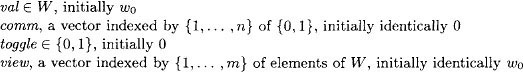
The handshake bits work as follows. There are now n + m shared variables: variables x(i), 1 ≤ i ≤ m as in the UnboundedSnapshot algorithm, plus new variables y(j), 1 ≤ j ≤ n. Each variable x(i) is writable by update process i and readable by all processes, as before. Each variable y(j), 1 ≤ j ≤ m, is writable by update process j (specifically, by the embedded-snap part of update process j) and is readable by all update processes, and each variable y(j), m + 1 ≤ j ≤ n, is writable by snap process j and readable by all update processes. Note that, unlike in the UnboundedSnapshot algorithm, the execution of the snap and embedded-snap operations in BoundedSnapshot involve writing to shared memory.
For each update process i, 1 ≤ i ≤ m, there are n pairs of handshake bits, one pair per process j. The pair of bits for (i, j) allow process i to tell process j about new updates by process i and also allow process j to acknowledge that it has seen this information. Specifically, x(i) contains a length n vector comm of bits, where the element comm(j) in variable x(i)—which we denote by x(i).comm(j)—is used by process i to communicate with process j about new updates by process i. And y(j) contains a length m vector ack of bits, where the element ack(i) in variable y(j)—which we denote by y(j).ack(i)—is used by process j to acknowledge that it has seen new updates by process i. Thus, the pair of handshake bits for (i, j) are x(i).comm(j) and y(j).ack(i).
The way these handshake bits are used is roughly as follows. When a process i executes an update(w), it begins by reading all the handshake bits y(j).ack(i). Then it performs its write to x(i); when it does this, it writes the value w and embedded snap response view, as it does in UnboundedSnapshot, and in addition writes the handshake bits in comm. In particular, for each j, it sets the bit comm(j) to be unequal to the value of y(j).ack(i) read at the beginning of the operation.
A process j performing a snap or embedded-snap repeatedly tries to perform two sets of reads, looking for the situation where nothing has changed in between the two sets of reads. But this time, changes are detected using the handshake bits rather than integer-valued tags. Specifically, before each attempt to find two consistent sets of reads, process j first reads all the handshake bits x(i).comm(j) and sets each handshake bit y(j).ack(i) equal to the value of x(i).comm(j) just read. (Thus, the update operations attempt to set the handshake bits unequal and the snap and embedded-snap operations attempt to set them equal.) Process j looks for changes to the handshake bits comm(j) in between its two sets of reads; if it finds such changes on 2m + 1 separate attempts, then it knows it has seen the results of four separate update operations by the same process i and can adopt the vector view produced by the third of these operations.
The handshake protocol described so far is simple and is “sound” in the sense that every time a process performing a snap or embedded-snap detects a change, a new update has in fact occurred. However, it turns out that the handshake is not sufficient to discover every update—it is possible for two consecutive updates by a process i not to be distinguished by some other process j. Consider, for example, the following situation.
Example 13.3.1 Insufficiency of handshake bits
Suppose that at some point during an execution, x(i).comm(j) = 0 and y(j).ack(i) = 1, that is, the handshake bits used to tell j about i’s updates are unequal. Then the following events may occur, in the indicated order. (The actions involving the two processes i and j appear in separate columns.)

In this sequence of events, process j performs three reads of x(i).comm(j). The first of these is just a preliminary test; the second and third are part of an attempt to find two consistent sets of reads. Here, process j determines as a result of its second and third reads that no updates have occurred in between. This is erroneous.
To overcome this problem, we augment the handshake protocol with a second mechanism: each x(i) contains an additional toggle bit that is flipped by process i during each of its write steps. This ensures that each update changes the value of the shared variable x(i). In a bit more detail, the protocol works as follows:
BoundedSnapshot algorithm:
Each shared variable x(i), 1 ≤ i ≤ m, is writable by process i and readable by all processes. It contains the following fields:
Also, each shared variable y(j), 1 ≤ j ≤ n, is writable by process j and readable by processes i, 1 ≤ i ≤ m. It contains the following field:
When a snapj input occurs on port j, m + ≤ j ≤ n, process j behaves as follows. It repeatedly attempts to obtain two sets of reads that look “consistent.” Specifically, in each attempt, process j first reads all the relevant handshake bits x(i).comm(j), for all i, 1 ≤ i ≤ m, in any order. Then for each i, process j sets y(j).ack(i) to be equal to the value read in x(i).comm(j); it does this in a single write step. Then process j performs two complete sets of reads, the first set finishing before the second set begins. If for every i, x(i).comm(j) and x(i).toggle are identical in the two reads of x(i), and, moreover, the common value of comm(j) is the same one that process j read at the beginning of this attempt, then the snap returns the vector of values x(i).val obtained in the final set of reads. Otherwise, process j records which variables x(i) have changed.
If process j ever records on three separate attempts that the same x(i) has changed, then consider the second of these three attempts. The snapj operation returns the vector of values in x(i).view obtained in the final read of x(i) at that attempt. (It is guaranteed that this vector was written in the course of an update operation whose interval is completely contained within the interval of the given snapj.)
When an update(w)i input occurs on port i, 1 ≤ i ≤ m, process i behaves as follows. First, it reads all the relevant handshake bits y(j).ack(i), 1 ≤ j ≤ n. Second, it performs an embedded-snap, which is the same as a snap except that the vector determined is not returned to the user. Third, process i performs a single write to x(i), setting the four fields of x(i) as follows:
- x(i).val := w
- For each j, x(i).comm(j) is set unequal to the value of y(j).ack(i) obtained in the initial read of y(j).
- x(i).toggle is set unequal to its previous value.
- x(i).view is set to the vector returned by the embedded-snap.
Finally, process i outputs acki.
Theorem 13.14 The BoundedSnapshot algorithm is a snapshot atomic object guaranteeing wait-free termination.
Proof Sketch. Well-formedness and wait-freedom are easy to see, as in the proof of Theorem 13.13 for the UnboundedSnapshot algorithm. It remains to show the atomicity condition. The argument is similar to that for UnboundedSnapshot.
Again, we fix execution α and (in view of Lemma 13.10) assume without loss of generality that α contains no incomplete operations. The serialization points are inserted exactly as for the UnboundedSnapshot algorithm. For example, for a snap or embedded-snap operation that terminates by finding two consistent sets of reads, we select any point between the end of the first of these two sets and the beginning of the second. As before, it is easy to see that the serialization points occur within the required intervals. It remains to show that the result of shrinking the operation intervals to their respective serialization points is a trace of the snapshot variable type. As before, it is enough to show that every completed snap and embedded-snap operation returns the correct vector after the prefix of α up to the serialization point.
This time, it is not so easy to show this property for snap and embedded-snap operations that terminate by finding two consistent sets of reads. To show this, it is enough to prove the following claim.
Claim 13.15 If a snap or embedded-snap terminates by finding two consistent sets of reads, then the following is true for all i. No write event by process i occurs between the read of x(i) in the first set and the read of x(i) in the second set.
Proof. By contradiction, using a somewhat detailed operational argument. Suppose that a snap on port j terminates by finding two consistent sets of reads, yet a write event by process i occurs between π1, the read of x(i) in the first set, and π2, the read of x(i) in the second set. (The argument is the same for an embedded-snap.) Let ϕ be the last such write, that is, the last write of x(i) prior to π2.
By the fact that the two sets of reads are consistent, the values of x(i).comm(j) read in π1 and π2 are equal and, moreover, are the same as the value last written in y(j).ack(i) before π1 (as part of process j’s successful attempt to find the consistent sets of reads). Let b denote this common value and let π0 denote this last write event. Also by consistency, the values of x(i).toggle read in π1 and π2 are equal. Let ![]() denote this common value.
denote this common value.
Since ϕ is the last write of x(i) prior to π2, it must be that it sets x(i).comm(j) := b and x(i).toggle := t. The update operation containing ϕ must contain an earlier read event ![]() of y(j). By the way update operations behave, the value of y(j).ack(i) read by
of y(j). By the way update operations behave, the value of y(j).ack(i) read by ![]() must be
must be ![]() (We are using the bar notation here to denote bit complementation.) This implies that
(We are using the bar notation here to denote bit complementation.) This implies that ![]() must precede π0.
must precede π0.
Thus, the order of the various read and write events must be the following. (Again, the actions involving the two processes i and j appear in separate columns.)
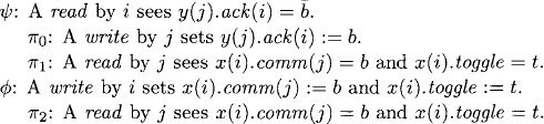
But note that the read event ![]() is part of the same update operation as the write event ϕ. This implies that the two read events π1 and π2 must be returning results written by two consecutive writes by process i. However, the toggle bits returned by π1 and π2 are identical, which contradicts the way the toggle bits are managed.
is part of the same update operation as the write event ϕ. This implies that the two read events π1 and π2 must be returning results written by two consecutive writes by process i. However, the toggle bits returned by π1 and π2 are identical, which contradicts the way the toggle bits are managed. ![]()
This shows Claim 13.15, which implies that every snap or embedded-snap operation that terminates by finding two consistent sets of reads in fact returns the correct vector after the prefix of α up to the serialization point. For the other snap and embedded-snap operations, the needed property is argued, as for UnboundedSnapshot, by induction on the number of response events for such operations in α.
Complexity analysis. The BoundedSnapshot algorithm uses n + m shared variables. Each variable x(i) takes on ![]() values, and each variable y(j) takes on 2m values. For time complexity, a non-failing process executing a snap makes at most 2m + 1 attempts to find two consistent sets of reads. For each attempt, there are at most 4m shared memory accesses, for a total time that is O (m2ℓ). The same bound holds for an update.
values, and each variable y(j) takes on 2m values. For time complexity, a non-failing process executing a snap makes at most 2m + 1 attempts to find two consistent sets of reads. For each attempt, there are at most 4m shared memory accesses, for a total time that is O (m2ℓ). The same bound holds for an update.
Using snapshots in programming read/write shared memory systems. Snapshot shared variables represent a powerful type of shared memory. For example, using a single snapshot shared variable, it is possible to simplify considerably the Bakery mutual exclusion algorithm of Section 10.7. We leave this for an exercise.
Using the techniques of Section 13.1.4 and a snapshot algorithm such as the ones in this section, an algorithm A that uses snapshot shared variables can be transformed into an algorithm that uses only single-writer/multi-reader read/write shared variables. This transformation requires some simple restrictions on A, as discussed in Section 13.1.4. (Also, technically, the snapshot atomic objects used in the transformation have one port corresponding to each process of A; process i of A might submit both update and snap operations on the same port i. But there is no problem in modifying the snapshot atomic object external interface and implementations to permit this.)
Read/update/snap variables. A useful variation on a snapshot shared variable, which only supports update and snap operations, is a read/update/snap shared variable, which supports read operations on individual locations in the shared vector in addition to snap operations returning the entire vector. Of course, a model using read/update/snap shared variables has no more power than a model using only snapshot variables, because a read can be implemented using a snap. However, the use of read/update/snap shared variables can allow more efficient programming, because it is possible to implement a read/update/snap atomic object so that the reads are very fast. We leave this for an exercise.
13.4 Read/Write Atomic Objects
Read/write shared variables (registers) are among the most basic building blocks used in shared memory multiprocessors. In this section, we consider the implementation of powerful multi-writer/multi-reader registers in terms of less powerful registers, such as single-writer/single-reader registers. More precisely, we consider the problem of implementing multi-writer/multi-reader read/write atomic objects using single-writer/single-reader shared variables.
13.4.1 The Problem
Fix a domain V and initial value v0 ∈ V.
In Example 13.1.1, we described an external interface for a l-writer/2-reader read/write atomic object for domain V. In general, an m-writer/p-reader read/write atomic object for domain V has an analogous external interface, where ports 1,…, m are write ports and ports m + 1,…, m + p are read ports. We again let n = m + p.
Since we consider the implementation of read/write atomic objects in terms of read/write shared variables, we need a way of distinguishing the high-level read and write operations that are submitted by the users at the ports from the low-level read and write operations that are performed on the read/write shared variables. We use the convention of capitalizing the names of the high-level operations. Thus, associated with port i, 1 ≤ i ≤ m, there are WRITE(v)i inputs, v ∈ V, and ACKi outputs, and associated with port j, m + 1 ≤ j ≤ n, there are READj inputs and Vj outputs, v ∈ V. (We don’t attempt to capitalize the values in V.) There are also STOPi inputs, 1 ≤ i ≤ n.
We consider implementing such an m-writer/p-reader atomic object, where n = m+p, using a shared memory system with n processes, one per port. We assume that all the shared variables in this system are read/write shared variables, but the numbers of readers and writers will vary in the different algorithms we present. All the implementations we describe guarantee wait-free termination.
13.4.2 Another Lemma for Showing Atomicity
We begin with a technical lemma that is useful for showing that a sequence β of actions of a read/write atomic object external interface satisfies the atomicity property for read/write objects. This lemma lists four conditions involving a partial order on operations in β. If an ordering satisfying these four conditions exists, it is guaranteed that there is some way to insert serialization points so as to satisfy the atomicity property. When reasoning about algorithms, it is often easier to show the existence of such a partial order than it is to explicitly define the serialization points.
Lemma 13.16 Let β be a (finite or infinite) sequence of actions of a read/write atomic object external interface. Suppose that β is well-formed for each i, and contains no incomplete operations. Let II be the set of all operations in β.
Suppose that ![]() is an irreflexive partial ordering of all the operations in II, satisfying the following properties:
is an irreflexive partial ordering of all the operations in II, satisfying the following properties:
- For any operation π ∈ II, there are only finitely many operations ϕ such that ϕ
 π.
π. - If the response event for π precedes the invocation event for ϕ in β, then it cannot be the case that ϕ π.
- If π is a WRITE operation in II and ϕ is any operation in II, then either π ϕ or ϕ π.
- The value returned by each READ operation is the value written by the last preceding WRITE operation according to (or v0, if there is no such WRITE).
Then β satisfies the atomicity property.
Condition 1 is a technical one, ruling out funny orderings in which infinitely many operations precede some particular other operation. Condition 2 says that the ![]() ordering must be consistent with the order of invocations and responses by the users. Condition 3 says that
ordering must be consistent with the order of invocations and responses by the users. Condition 3 says that ![]() totally orders all the WRITE operations and orders all the READ operations with respect to the WRITE operations. Condition 4 says that the responses to READs are consistent with
totally orders all the WRITE operations and orders all the READ operations with respect to the WRITE operations. Condition 4 says that the responses to READs are consistent with ![]() .
.
Proof. We describe how to insert a serialization point *π for every operation π ∈ II. Namely, we insert each serialization point *π immediately after the latest of the invocations for π and for all the operations ϕ such that ϕ ![]() π. Condition 1 implies that this position is well-defined. We order *’s that are thereby placed contiguously in any way that is consistent with the ordering
π. Condition 1 implies that this position is well-defined. We order *’s that are thereby placed contiguously in any way that is consistent with the ordering ![]() on the associated operations; that is, if π and ϕ are two operations whose *’s are placed contiguously, and if ϕ
on the associated operations; that is, if π and ϕ are two operations whose *’s are placed contiguously, and if ϕ ![]() π, then *ϕ precedes *π.
π, then *ϕ precedes *π.
We claim that the total order of the serialization points is consistent with ![]() ; that is, for any operations π and ϕ in II, if ϕ
; that is, for any operations π and ϕ in II, if ϕ ![]() π, then *ϕ precedes *π. To see this, assume that ϕ
π, then *ϕ precedes *π. To see this, assume that ϕ ![]() π. By construction, *ϕ is placed after the latest of the invocations for ϕ and for all the operations that precede ϕ in the
π. By construction, *ϕ is placed after the latest of the invocations for ϕ and for all the operations that precede ϕ in the ![]() order. And *π is placed after the latest of the invocations for π and for all the operations that precede π in the
order. And *π is placed after the latest of the invocations for π and for all the operations that precede π in the ![]() order. But since ϕ
order. But since ϕ ![]() π, it follows that any operation that precedes ϕ in
π, it follows that any operation that precedes ϕ in ![]() also precedes π in
also precedes π in ![]() . Since a tie would be broken by ordering *ϕ before *π, it follows that *ϕ precedes *π, as claimed.
. Since a tie would be broken by ordering *ϕ before *π, it follows that *ϕ precedes *π, as claimed.
Next, we claim that these serialization points are within the required intervals. To see this, consider any operation π ∈ II. By construction, the serialization point *π for π must appear after the invocation for π. We show that *π appears before the response for π. Suppose for the sake of contradiction that it appears after the response for π. Then, by construction, this means that the response for π must precede (in β) the invocation for some operation ϕ, where ϕ ![]() π. But this contradicts Condition 2.
π. But this contradicts Condition 2.
It remains to show that the result of shrinking the operation intervals to their serialization points is a trace of the underlying read/write variable type. This means that each READ operation π returns the value of the WRITE whose serialization point is the last one before *π (or v0, if there is no such WRITE).
But Condition 3 says that ![]() orders all the WRITE operations in II with respect to all operations in II. And by Condition 4 for READ operations, the value returned by any READ operation π is the value written by the last preceding WRITE operation according to
orders all the WRITE operations in II with respect to all operations in II. And by Condition 4 for READ operations, the value returned by any READ operation π is the value written by the last preceding WRITE operation according to ![]() (or v0, if there is no such WRITE). Since the total order of the serialization points is consistent with
(or v0, if there is no such WRITE). Since the total order of the serialization points is consistent with ![]() , it follows that π returns the required value.
, it follows that π returns the required value.
In the rest of this section, we use Lemma 13.16 to show that objects guarantee the atomicity condition.
13.4.3 An Algorithm with Unbounded Variables
Our first algorithm is the VitanyiAwerbuch algorithm, which implements m-writer/p-reader read/write atomic objects using single-writer/single-reader registers. (Recall that n = m+p.) This algorithm is simple but has the disadvantage that the shared variables are unbounded in size.
VitanyiAwerbuch algorithm:
The algorithm uses n2 shared variables, which we can imagine to be arranged in an n x n matrix X, as depicted in Figure 13.9. The variables are named x(i, j): 1 ≤ i, j ≤ n. Each variable x(i, j) is readable only by process i and writable only by process j; thus, each process i can read all the variables in row i and can write all the variables in column i of X.
Each shared register x(i, j) has the following fields:
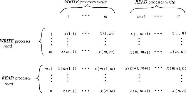

We use the abbreviation tagpair for the pair (tag, index). We order tagpairs lexicographically.
When a WRITE(v)i input occurs, process i behaves as follows. First, it reads all the variables x(i, j), 1 ≤ j ≤ n (in any order). Let k be the greatest tag it finds. Next, process i performs a single write to each x(j, i), 1 ≤ j ≤ n, setting the three fields of x(j, i) as follows:
- x(j, i).val := v
- x(j, i).tag := k + 1
- x(j, i).index := i
Finally, process i outputs ACKi.
When a READi input occurs, process i behaves as follows. First, it reads all the variables x(i, j), 1 ≤ j ≤ n (in any order). Let (v, k, j) be any (val, tag, index) triple it finds with maximum tagpair = (tag, index). Next, process i performs a single write to each x(j, i), 1 ≤ j ≤ n, setting the three fields of x(j, i) as follows:
(That is, it propagates the best information it has read to all the variables it can write.) Finally, process i outputs Vi (i.e., outputs value v on port i).
Theorem 13.17 The VitanyiAwerbuch algorithm is a read/write atomic object guaranteeing wait-free termination.
In order to prove the correctness of the VitanyiAwerbuch algorithm, we could proceed as in the proofs for the snapshot algorithms, explicitly inserting serialization points and then showing that the atomicity property is satisfied. However, for the VitanyiAwerbuch algorithm, it is not easy to see (as it is for the earlier algorithms) exactly where the serialization points ought to be placed. A more natural proof strategy here is to establish a partial order of operations based on the tagpair values, and then show that this partial order satisfies the conditions of Lemma 13.16.
Proof. Well-formedness and wait-free termination are easy to see. For atomicity, we use Lemma 13.16.
Let α be any execution of the VitanyiAwerbuch algorithm. In view of Lemma 13.10, we may assume without loss of generality that α contains no incomplete operations. We begin with a simple claim.
Claim 13.18 For any variable x(i, j), the tagpair = (tag, index) values are monotone nondecreasing in α.
Proof. Fix i and j. Note that variable x(i, j) is written only by process j and that, by well-formedness, all operations by j must occur sequentially. Also, after any number of complete operations by j, all the variables in the jth column contain the same tagpair.
Each time j performs an operation, it starts by reading all variables in the jth row, including the “diagonal” variable x(j, j). The tagpair that it writes is then chosen to be at least as large as the tagpair that it finds in x(j, j). But this is the same as the tagpair in x(i, j) prior to the operation. So the tagpair in x(i, j) after the operation is at least as large as before the operation. This is enough to show the claim.
Next, define II to be the set of operations occurring in α. For every (WRITE or READ) operation π ∈ II, we define tagpair(π) to be the unique tagpair value that it writes.
Claim 13.19 All tagpair(π) values for distinct WRITE operations in α are distinct.
Proof. For WRITE operations on different ports this is certainly true, since the index fields of the tagpairs are different.
So consider operations on the same port; by well-formedness, these operations occur sequentially. Let π and ϕ be two WRITE operations on port i and assume without loss of generality that π precedes ϕ. Then π completes writing to all the variables in the ith column before ϕ begins reading the variables in the ith row. In particular, ϕ sees, in the “diagonal” variable x(i, i), a tagpair written by π or a later operation. By Claim 13.18, this tagpair is at least as large as that of π. Then ϕ chooses a larger, and hence a different, tagpair for itself.
Now we define a partial ordering on operations in II. Namely, we say that π ![]() ϕ exactly if either of the following applies:
ϕ exactly if either of the following applies:
- tagpair(π) < tagpair(ϕ)
- tagpair(π) = tagpair(ϕ), π is a WRITE and ϕ is a READ
It is enough to verify that this satisfies the four conditions needed for Lemma 13.16 (where β = trace(α) = α|ext(A x U)).
1. For any operation π ∈ II, there are only finitely many operations ϕ such that ϕ ![]() π.
π.
Suppose for the sake of contradiction that operation π has infinitely many ![]() predecessors. Claim 13.19 implies that it cannot have infinitely many predecessors that are WRITE operations, so it must have infinitely many predecessors that are READ operations. Without loss of generality, we may assume that π is a WRITE.
predecessors. Claim 13.19 implies that it cannot have infinitely many predecessors that are WRITE operations, so it must have infinitely many predecessors that are READ operations. Without loss of generality, we may assume that π is a WRITE.
Then there must be infinitely many READ operations with the same tagpair, t, where ![]() is smaller than tagpair(π). But the fact that π completes in α implies that tagpair(π) eventually gets written to some variable in each row. After this happens, Claim 13.18 implies that any READ operation that is subsequently invoked is guaranteed to see, and thus to obtain, a tagpair that is ≥ tagpair(π) > t. This contradicts the existence of infinitely many READ operations with tagpair t.
is smaller than tagpair(π). But the fact that π completes in α implies that tagpair(π) eventually gets written to some variable in each row. After this happens, Claim 13.18 implies that any READ operation that is subsequently invoked is guaranteed to see, and thus to obtain, a tagpair that is ≥ tagpair(π) > t. This contradicts the existence of infinitely many READ operations with tagpair t.
2. If the response event for π precedes the invocation event for ϕ in β, then it cannot be the case that ϕ ϕ ![]() π.
π.
Suppose that π’s response precedes the invocation of ϕ. When π completes, its tagpair has been written to all its column variables. Thus by Claim 13.18, when ϕ reads its row variables, it reads a tagpair that is at least as large as tagpair(π). Therefore, tagpair(ϕ) is chosen to be at least as large as tagpair(π). Moreover, if ϕ is a WRITE operation, then tagpair(ϕ) is chosen to be strictly greater than tagpair(π).
Since tagpair(π) ≤ tagpair(ϕ), the only way we could have ϕ ![]() π is if tagpair(π) = tagpair(ϕ), π is a READ operation and ϕ is a WRITE operation. But this is not possible, because if ϕ is a WRITE, then, as noted above, we have tagpair(ϕ) > tagpair(π). So it is not the case that ϕ
π is if tagpair(π) = tagpair(ϕ), π is a READ operation and ϕ is a WRITE operation. But this is not possible, because if ϕ is a WRITE, then, as noted above, we have tagpair(ϕ) > tagpair(π). So it is not the case that ϕ ![]() π.
π.
3. If π is a WRITE operation in II and ϕ is any operation in II, then either π ![]() ϕ Or ϕ
ϕ Or ϕ ![]() π.
π.
By Claim 13.19, all WRITE operations obtain distinct tagpairs. This implies that all of the WRITEs are totally ordered and also that each READ is ordered with respect to all the WRITEs.
4. The value returned by each READ operation is the value written by the last preceding WRITE operation according to ![]() (or v0, if there is no such WRITE).
(or v0, if there is no such WRITE).
Let π be a READ operation. The value v returned by π is just the value that π finds associated with the largest tagpair, t, among the variables in its row; this ![]() also becomes the tagpair of π. There are two cases:
also becomes the tagpair of π. There are two cases:
(a) Value v has been written by some WRITE operation ϕ with tagpair t.
In this case, the ordering definition ensures that ϕ is the last WRITE preceding π in the ![]() order, as needed.
order, as needed.
(b) v = v0 and ![]() = 0.
= 0.
In this case, the ordering definition ensures that there are no WRITEs preceding π in the ![]() order, as needed.
order, as needed.
Complexity analysis. The VitanyiAwerbuch algorithm uses n2 shared variables, each of unbounded size, even if the underlying domain V is finite. Each READ and each WRITE that completes involves 4n shared memory accesses, for a total time complexity that is O (nℓ).
13.4.4 A Bounded Algorithm for Two Writers
Like the UnboundedSnapshot algorithm, the VitanyiAwerbuch algorithm has the disadvantage that it uses unbounded-size shared variables to store unbounded tags. Many alternative algorithms have been designed that use only bounded data, but unfortunately, most are rather complicated (as well as too inefficient to be practical). In this section, we present only one very simple algorithm, for a special case.

Namely, we describe the Bloom algorithm for implementing a 2-writer/p-reader read/write atomic object using two 1-writer/p + 1-reader registers, x(1)> and x(2). (Now n = 2 + p.) Each x(i) is writable by WRITE process i and readable by all the other processes. Figure 13.10 depicts the architecture for the special case of two readers. The algorithm is simple but does not have an apparent generalization to more writers.
Bloom algorithm:
The algorithm uses two shared variables, x(1) and x(2), where x(i) is writable by process i and readable by all other processes. Here let ī denote 2 if i = 1, and 1 if i = 2. Register x(i) has the following fields:
When a WRITE(v)i occurs on port i, i ∈ {1, 2}, process i behaves as follows. First, it reads x(ī); let b be the tag it finds there. Then it writes x(i), setting the fields as follows:
- x(i).val := v
- x(i).tag := b + i mod 2
Thus, when a WRITE process i performs a WRITE, it not only writes the new value into its variable, but it also attempts to make the sum of the tags in the two variables equal to its own index, modulo 2. That is, process 1 always tries to make the tags in the two variables unequal, while process 2 tries to make them equal.
When a READi occurs on port i, 3 ≤ i ≤ n, process i behaves as follows. First, it reads both registers; let b be the sum modulo 2 of the two tags that it finds there. Then it rereads register x(1) if b = 1 and register x(2) if b = 0, and returns the val that it finds there.
Thus, all READ processes behave in exactly the same way. Each READ process reads both registers to determine whether they contain equal or unequal tags. If the tags are equal, the process obtains its return value from x(2), and otherwise from x(1).
Theorem 13.20 The Bloom algorithm is a read/write atomic object guaranteeing wait-free termination.
Once again, in order to prove correctness, we could proceed by explicitly inserting serialization points and then showing that the atomicity property is satisfied. However, this time we use an interesting strategy based on a combination of Lemma 13.16 and a simulation proof, as defined in Section 8.5.5. We first define a variant of the Bloom algorithm, IntegerBloom, which uses integer-valued tags instead of bits. We show that IntegerBloom is correct, using Lemma 13.16. Then we show that Bloom is correct by using a simulation relation from Bloom to IntegerBloom.
IntegerBloom algorithm:
The algorithm uses two shared variables, x(1) and x(2), where x(i) is writable by process i and readable by all other processes. Register x(i) has the following fields:
When a WRITE(v)i occurs on port i, i ∈ {1,2}, process i behaves as follows. First, it reads x(ī); let ![]() be the tag it finds there. Then it writes x(i), setting the fields as follows:
be the tag it finds there. Then it writes x(i), setting the fields as follows:
- x(i).val := v
- x(i).tag := + 1
When a READi occurs on port i, 3 ≤ i ≤ n, process i behaves as follows. First, it reads both registers; let ![]() 1 and
1 and ![]() 2 be the respective tags it finds there. Then there are two cases: If |
2 be the respective tags it finds there. Then there are two cases: If |![]() 1 −
1 − ![]() 2| ≤ 1, then process i rereads the register holding the greater tag and returns the val that it finds there. (This register must be uniquely defined, because, as we state in Lemma 13.21 below, the tags in x(1) are always even and the tags in x(2) are always odd.) Otherwise—that is, if |
2| ≤ 1, then process i rereads the register holding the greater tag and returns the val that it finds there. (This register must be uniquely defined, because, as we state in Lemma 13.21 below, the tags in x(1) are always even and the tags in x(2) are always odd.) Otherwise—that is, if |![]() 1 −
1 − ![]() 2| > 1—process i nondeterministically chooses either register to reread and returns the val that it finds there.
2| > 1—process i nondeterministically chooses either register to reread and returns the val that it finds there.
The following lemma gives some basic properties of IntegerBloom. It is easy to prove.
Lemma 13.21 In any reachable state of IntegerBloom, the following are true:
- x(1).tag is even.
- x(2).tag is odd.
- 3. |x(1).tag − x(2).tag| ≤ 1.
Theorem 13.22 The IntegerBloom algorithm is a read/write atomic object guaranteeing wait-free termination.
Proof. Similar to the proof of Theorem 13.17. Well-formedness and wait-free termination are easy to see. For atomicity, we use Lemma 13.16. Let α be any execution of the IntegerBloom algorithm. As before, we assume without loss of generality that α contains no incomplete operations.
Claim 13.23 For each variable x(i), the tag values are monotone nondecreasing in α.
Let II denote the set of operations occurring in α. For every WRITE operation π in II, we define tag(π) to be the tag value written by π in its write step.
Now we define a partial ordering on operations in II. First, we order the WRITE operations by their tag values. If two WRITE operations have the same tag, then they must belong to the same writer, and we order them in the order in which they occur. Next, we order each READ operation in II just after the WRITE whose value it obtains (or before all the WRITEs, if there is no such WRITE).
It is enough to verify that this satisfies the four conditions needed for Lemma 13.16 (where β = trace(α) = α|ext(A x U)). Conditions 3 and 4 are immediate, so all we must show are Conditions 1 and 2. For these, the following is useful:
Claim 13.24 If the write step of WRITE operation π precedes the invocation of WRITE operation ϕ, then π ![]() ϕ.
ϕ.
Proof. If π and ϕ occur on the same port, then Claim 13.23 implies that tag(π) ≤ tag(ϕ), and the definition of ![]() implies that π
implies that π ![]() ϕ. On the other hand, if π and ϕ occur on different ports, then ϕ reads the result of either π or a later WRITE on π’s port. By Claim 13.23, the tag read by ϕ is greater than or equal to tag(π). Therefore, tag(π) < tag(ϕ), so again π
ϕ. On the other hand, if π and ϕ occur on different ports, then ϕ reads the result of either π or a later WRITE on π’s port. By Claim 13.23, the tag read by ϕ is greater than or equal to tag(π). Therefore, tag(π) < tag(ϕ), so again π ![]() ϕ.
ϕ. ![]()
Claim 13.25 If the write step of WRITE operation π precedes the invocation of READ operation ϕ, then π ![]() ϕ.
ϕ.
Proof. We must show that ϕ returns the result of π or of some other WRITE ![]() with π
with π ![]()
![]() . Let
. Let ![]() = tag(π) and suppose that π occurs on port i.
= tag(π) and suppose that π occurs on port i.
When ϕ is invoked, Claim 13.23 implies that x(i).tag ≥ ![]() , and Lemma 13.21 implies that |x(1).tag − x(2).tag| ≤ 1. Therefore, when ϕ is invoked, x(ī).tag ≥
, and Lemma 13.21 implies that |x(1).tag − x(2).tag| ≤ 1. Therefore, when ϕ is invoked, x(ī).tag ≥ ![]() − 1. By the definition of
− 1. By the definition of ![]() and Claim 13.23, the only problem is if ϕ returns the value of some WRITE with tag =
and Claim 13.23, the only problem is if ϕ returns the value of some WRITE with tag = ![]() − 1. So suppose this is the case.
− 1. So suppose this is the case.
Then ϕ must see x(ī).tag = ![]() − 1 on either its first or its second read, and again on its third read. If ϕ sees x(ī).tag =
− 1 on either its first or its second read, and again on its third read. If ϕ sees x(ī).tag = ![]() on either its first or second read, then the combination of tags t − 1 and
on either its first or second read, then the combination of tags t − 1 and ![]() causes ϕ to choose to reread register x(ī) rather than register x(ī), a contradiction. So it must be that ϕ sees x(i).tag > t. But Lemma 13.21 implies that by the time ϕ sees x(i).tag >
causes ϕ to choose to reread register x(ī) rather than register x(ī), a contradiction. So it must be that ϕ sees x(i).tag > t. But Lemma 13.21 implies that by the time ϕ sees x(i).tag > ![]() , it must also be the case that x(ī) >
, it must also be the case that x(ī) > ![]() − 1. This means that ϕ cannot see x(ī) =
− 1. This means that ϕ cannot see x(ī) = ![]() − 1 on its third read, again a contradiction.
− 1 on its third read, again a contradiction. ![]()
Using Claims 13.24 and 13.25, Condition 1 is easy to show; we leave this for an exercise.
For Condition 2, suppose that the response event for π precedes the invocation for ϕ in β. If π is a WRITE, then Claims 13.24 and 13.25 imply that π ![]() ϕ. So suppose that π is a READ. Suppose for the sake of contradiction that ϕ
ϕ. So suppose that π is a READ. Suppose for the sake of contradiction that ϕ ![]() π.
π.
If ϕ is a WRITE, then clearly π cannot return the result of ϕ, since ϕ does not perform its write step until after ϕ has completed. So the only problem is if π returns the result of some WRITE ![]() , where ϕ
, where ϕ ![]()
![]() . But in this case, the write step within
. But in this case, the write step within ![]() precedes the end of π and so precedes the invocation of ϕ. But then Claim 13.24 implies that
precedes the end of π and so precedes the invocation of ϕ. But then Claim 13.24 implies that ![]()
![]() ϕ, a contradiction.
ϕ, a contradiction.
On the other hand, if ϕ is a READ, then the assumption that ϕ ![]() π implies that there must be some WRITE operation
π implies that there must be some WRITE operation ![]() such that ϕ
such that ϕ ![]()
![]() and π obtains the result of
and π obtains the result of ![]() . Since π obtains the result of
. Since π obtains the result of ![]() , it must be that the write step within
, it must be that the write step within ![]() precedes the end of π and so precedes the invocation of ϕ. But then Claim 13.25 implies that
precedes the end of π and so precedes the invocation of ϕ. But then Claim 13.25 implies that ![]()
![]() ϕ, again a contradiction.
ϕ, again a contradiction.
Now we show the correspondence between the Bloom and IntegerBloom algorithms, using a simulation relation. The general strategy is described in Section 8.5.5 and is used in other proofs in Example 8.5.6 and in Section 10.9.4.
The correspondence between the two algorithms turns out (strangely enough) to be that the {0, 1}-valued tags used in the Bloom algorithm are the second-lowest-order bits of the integer-valued tags in the IntegerBloom algorithm.
Example 13.4.1 Bits versus integers in the Bloom algorithm
Consider an execution of IntegerBloom in which WRITE operations alternate on ports 1 and 2, beginning with port 1; each WRITE begins only after the previous one has completed. Then each WRITE produces a successively larger tag. The tag values in the two registers, written in binary notation, are shown in Figure 13.11. Initially, x(1) and x(2) start with tags 0 and 1, respectively. The first WRITE1 sets x(1).tag := 2, and then a WRITE2 sets x(2).tag := 3, and so on.
In the corresponding execution of Bloom, the tag values in the two registers are as shown in Figure 13.12. Initially, both registers start with tag = 0. Each WRITE1 sets x(1).tag to be unequal to x(2).tag, while each WRITE2 sets x(2).tag to be equal to x(1).tag.
Notice that in each case, the tag in the Bloom execution is just the second-lowest-order bit of the corresponding tag in the IntegerBloom execution.
It turns out that the correspondence illustrated in Example 13.4.1 holds in all executions of the two algorithms. If s and u are states of the Bloom and IntegerBloom systems (algorithms plus users), respectively, then we define (s, u) ∈ f (or u ∈ f(s)), provided that all state components are identical, except that wherever u has an integer-valued tag, t, s has a bit-valued tag whose value is the second-lowest-order bit of t.


Lemma 13.26 f is a simulation relation from Bloom to IntegerBloom.
Proof Sketch. Since the unique initial states of the two algorithms are related by f, the start condition of the simulation definition is straightforward. The interesting thing to show is the step condition. It is enough to show that for any step (s, π, s′) of Bloom and any u ∈ f(s), where s and u are reachable states, there is a corresponding step (u, ϕ, u′) of Integer Bloom, where u′ ∈ f(s′) and ϕ is “almost” the same as π. Specifically, ϕ is the same as π except that it can involve an integer value, whereas π involves the second-lowest-order bit. We consider cases, based on π. If π is an invocation or response event, then the arguments are straightforward. The interesting steps are the write steps within the WRITE operations and the third read steps within the READ operations.
So suppose that (s, π, s′) is a step of Bloom in which process 1 writes x(1) as part of a WRITE1 operation. Then process 1 sets x(1).tag to be unequal to the value b that it remembers reading from x(2).tag. That is, s’.x(1).tag ≠ b. In the corresponding state u of IntegerBloom, process i remembers reading an integer-valued tag t from x(2).tag; since u ∈ f(s), it must be that b is the second-lowest-order bit of t. Let u′ be the unique state that results in IntegerBloom. Then u′.x(1).tag = ![]() + 1. To see that u′ ∈ f(s′), we need to show that the second-lowest-order bit of u′.x(1).tag is equal to s’.x(1).tag, that is, that the second-lowest-order bit of
+ 1. To see that u′ ∈ f(s′), we need to show that the second-lowest-order bit of u′.x(1).tag is equal to s’.x(1).tag, that is, that the second-lowest-order bit of ![]() + 1 is unequal to b. But this follows from the fact that
+ 1 is unequal to b. But this follows from the fact that ![]() is odd (by Lemma 13.21) and the fact that b is the second-lowest-order bit of t.
is odd (by Lemma 13.21) and the fact that b is the second-lowest-order bit of t.
The argument for the case where (s, π, s′) is a step in which process 2 writes x(2) is similar.
Now suppose that (s, π, s′) is a step of Bloom at which process i performs the third read step within a READ. The key claim is that IntegerBloom permits process i to read the same register, x(1) or x(2). Suppose that, in state s, the tags that process i of Bloom remembers reading in x(1) and x(2) are b1 and b2, respectively; likewise, suppose that in state u, the tags that process i of IntegerBloom remembers reading in x(1) and x(2) are ![]() 1 and
1 and ![]() 2, respectively.
2, respectively.
Since u ∈ f(s), we know that b1 is the second-lowest-order bit of ![]() 1 and b2 is the second-lowest-order bit of
1 and b2 is the second-lowest-order bit of ![]() 2. There are three cases.
2. There are three cases.
- 1 = 2 + 1.
Then Lemma 13.21 implies that the second-lowest-order bits of
1 and 2 are unequal. In this case, both Bloom and IntegerBloom read from register x(1). - 2 = 1 + 1.
Then Lemma 13.21 implies that the second-lowest-order bits of
1 and 2 are equal. In this case, both Bloom and IntegerBloom read from register x(2). - 1 ≠ 2 + 1 and 2 ≠ 1 + 1.
Then Lemma 13.21 implies that |![]() 1 −
1 − ![]() 2| > 1. In this case, IntegerBloom permits either register to be read.
2| > 1. In this case, IntegerBloom permits either register to be read.
Now we can prove Theorem 13.20, which asserts the correctness of the Bloom algorithm.
Proof (of Theorem 13.20). Lemma 13.26 and Theorem 8.12 imply that every trace of the Bloom system is a trace of the IntegerBloom system. (Recall that traces here include invocation and response events on ports, plus the stop events.) Theorem 13.22 implies that the well-formedness and atomicity conditions hold for IntegerBloom. Since the well-formedness and atomicity conditions are expressible as properties of traces, they carry over to the Bloom algorithm. Wait-free termination is easy to see.
Complexity analysis. The Bloom algorithm uses two shared variables, each of which can take on 2|V| values. Each operation requires only a constant number of shared memory accesses, or time O (ℓ).
13.4.5 An Algorithm Using Snapshots
In this final subsection, we give an implementation, SnapshotRegister, of a wait-free m-writer/p-reader read/write atomic object using a snapshot shared variable. (Again, let n = m + p.) Combining SnapshotRegister with the implementations of snapshot atomic objects in Section 13.3, using Corollary 13.9, yields implementations of wait-free m-writer/p-reader atomic objects using 1-writer/n-reader shared registers.
The snapshot shared variable used by SnapshotRegister has unbounded size, even if the underlying domain V for the read/write atomic object being implemented is bounded. It is possible, though quite difficult, to modify the Snapshot-Register algorithm to use a bounded snapshot shared variable.
SnapshotRegister algorithm:
The algorithm uses a single shared variable x, which is a snapshot object based on a length m vector. The domain W for each component of x consists of pairs (val, tag), where val ∈ V and tag ∈ ![]() ; the initial value w0 is (v0, 0).
; the initial value w0 is (v0, 0).
Each WRITE process i, 1 ≤ i ≤ m, performs update(i, w) and snap operations on x, while each READ process i, m + 1 ≤ i ≤ n, performs only snap operations on x.
When a READi input occurs on port i, m + 1 ≤ i ≤ n, process i behaves as follows. First, it performs a snap operation on x, thereby determining a vector u. Let j be the index, 1 ≤ j ≤ m, such that the pair (u(j).tag, j) is largest, in the lexicographic ordering of pairs. Then process i returns the associated value u(j).val.
When a WRITE(v)i input occurs on port i, 1 ≤ i ≤ m, process i behaves as follows. First, it performs a snap operation on x, thereby determining a vector u. As above, let j be the index, 1 ≤ j ≤ m, such that the pair (u(j).tag, j) is largest, in the lexicographic ordering of pairs. Then process i performs an update(i, (v, u(j).tag + 1)). Finally, process i outputs ACKi.
The SnapshotRegister algorithm is somewhat similar to the VitanyiAwerbuch algorithm, but it is simpler because of the extra power provided by the snapshot shared memory.
Theorem 13.27 The SnapshotRegister algorithm is a read/write atomic object guaranteeing wait-free termination.
Proof Sketch. This is similar to the proofs for VitanyiAwerbuch and Integer-Bloom, using Lemma 13.16, but simpler. We leave it as an exercise.
Complexity analysis. The SnapshotRegister algorithm uses one snapshot shared variable, which is of unbounded size, even if the underlying domain V is finite. Each operation requires only a constant number of shared memory accesses, for a total time that is O (ℓ).
Hierarchical construction. Theorem 13.27 and any wait-free implementation of the snapshot atomic object together yield a wait-free implementation of an m-writer/p-reader read/write atomic object using 1-writer/m + p-reader shared registers. The proof is based on Corollary 13.9. (Technically, in order to apply Corollary 13.9, we need a snapshot atomic object with only n = m + p ports, one per process—for example, WRITE process i should perform both its update and snap operations on the same port. There is no problem modifying the snapshot atomic object external interface and implementations to permit this.)
Generalizations. There are several interesting generalizations of the Snapshot-Register algorithm that also work correctly. First, during a WRITEi, if i = j—that is, if process i itself has the largest tag pair—then i may optionally use the same tag that it previously had. Second, it is possible to use nonnegative real-valued tags rather than integer-valued tags. Then the tag chosen by a writer i can be any real number that is strictly greater than the largest tag it sees. Once again, if i itself has the greatest tag pair, then it can reuse its previous tag. Both of these generalizations are useful for proving the correctness of other implementations of read/write atomic objects using a snapshot shared variable.
13.5 Bibliographic Notes
The idea of an “atomic object” appears to have originated with the work of Lamport [181, 182] on read/write atomic objects. Herlihy and Wing [153] extended the notion of atomicity to arbitrary variable types and renamed it linearizability. König’s Lemma was originally proved by König [170]; a proof appears in Knuth’s book [169]. The canonical wait-free atomic object automaton is derived from the work of Merritt, described in [3]. The connection between atomic objects and shared variables is derived from work by Lamport and Schneider [186] and by Goldman and Yelick [139]. The impossibility of implementing read-modify-write atomic objects using read/write objects is due to Herlihy [150].
The idea of a snapshot atomic object is due to Afek, Attiya, Dolev, Gafni, Merritt, and Shavit [3] and to Anderson [11, 12], inspired by the work of Chandy and Lamport on consistent global snapshots in distributed networks [68]. The snapshot atomic object implementations presented here, both Unbounded-Snapshot and BoundedSnapshot, are due to Afek, et al. The handshake strategy used in the BoundedSnapshot protocol is due to Peterson [240]. A more recent atomic snapshot algorithm, requiring only O (nl log n) time rather than quadratic time, has been developed by Attiya and Rachman [26].
Many algorithms have been designed for implementing read/write atomic objects in terms of simpler kinds of read/write registers. The VitanyiAwerbuch algorithm appears in a paper by Vitanyi and Awerbuch [283]; that paper also contains an algorithm using bounded shared variables, but that algorithm is incorrect. The Bloom algorithm is due to Bloom [53], and the SnapshotRegister algorithm is derived from work by Gawlick, Lynch, and Shavit [135]. Bounded algorithms for implementing single-writer/multi-reader atomic objects using single-writer/single-reader registers have been designed by Singh, Anderson, and Gouda [263] and Haldar and Vidyasankar [144]. Bounded algorithms for implementing multi-writer/multi-reader atomic objects using single-writer/multi-reader registers have been designed by Peterson and Burns [241]; Schaffer [254]; Israeli and Li [162]; Li, Tromp, and Vitanyi [196]; and Dolev and Shavit [100]. In particular, Schaffer’s algorithm corrects errors in Peterson and Burns’s algorithm. Gawlick, Lynch, and Shavit [135] describe an implementation of multi-writer/multi-reader atomic objects using a bounded snapshot variable and prove the correctness of this algorithm by a simulation proof, relating it to the generalized version of the SnapshotRegister algorithm. Several of these constructions use a notion of “bounded timestamping.” Bounded timestamping algorithms have been given by Israeli and Li [162]; Dolev and Shavit [100]; Gawlick, Lynch, and Shavit [135]; Israeli and Pinchasov [163]; Dwork and Waarts [107]; and Dwork, Herlihy, Plotkin, and Waarts [102].
Attiya and Welch have compared the costs of implementing read/write atomic objects with those of implementing read/write objects with slightly weaker consistency requirements [28]. Their work is carried out in the asynchronous network model.
13.6 Exercises
13.1. Define the external interface for a 2-writer/1-reader atomic object and give several interesting examples of sequences for this external interface that satisfy the atomicity property, as well as sequences that do not satisfy the atomicity property. Be sure to include both finite and infinite sequences, as well as sequences that contain incomplete operations.
13.2. Consider a read-modify-write atomic object whose domain V is the set of integers and whose initial value is 0. (See Section 9.4 for the definition of a read-modify-write variable type—recall that the return value for a read-modify-write shared variable is the value of the variable prior to the operation.)
The object has two ports: port 1 supports increment operations (which add 1 to the value in the object) only and port 2 supports decrement operations (which subtract 1) only. Which of the following sequences satisfy the atomicity property?
(a) increment1, decrement2, 01,02
(b) increment1, decrement2, − 11, 02
(c) increment1, decrement2, 01, 12
(d) decrement2, increment1, 01, increment1, 11 increment1, 21, increment1, 31, …
(e) decrement2, increment1, 01, increment1, 01, increment1, 11, increment1, 21, …
13.3. Fill in some more details in the proof of Theorem 13.1. In particular, show in more detail than we have in the text that there are arbitrarily long paths from the root and that an infinite path yields a correct selection for the entire sequence β.
13.4. Generalize the definition of a variable type to allow finitely many initial values rather than just one and to allow finite nondeterministic choice rather than just a function. Generalize Theorem 13.1 and its proof to this new setting. What happens if we allow infinite nondeterminism?
13.5. Suppose that we modify Example 13.1.4 so that the system supports decrement operations as well as read and increment operations. The algorithm is the same as before, with the following addition: when a decrementi input occurs on port i, process i decrements x(i).
Is the resulting system a read/increment/decrement atomic object? Either prove that it is or give a counterexample execution.
13.6. Prove Theorem 13.4.
13.7. Prove Theorem 13.5.
13.8. Prove Theorem 13.6.
13.9. Show that Theorem 13.7 is false if we do not include the special assumption about A’s turn function.
13.10. Give a formal description, using precondition-effect notation, of the RMWfromRW algorithm. Your description should be modular in that it should represent the mutual exclusion component as a separate automaton, combined with the main portion of the RMWfromRW algorithm using I/O automaton composition. Prove that your algorithm works correctly (assuming the correctness properties of the mutual exclusion component).
13.11. Consider a modification of the UnboundedSnapshot algorithm in which each snap and embedded-snap looks for three different tags for some x(i) rather than four as described. Is the modified algorithm still correct? Either prove that it is or give a counterexample execution.
13.12. Consider a modification of the UnboundedSnapshot algorithm in which process i increments x(i).tag when it performs a snap operation, as well as when it performs an update operation. (The x(i).val and x(i).view components are not changed, and the embedded-snap operation is not modified in any way.)
Is the modified algorithm still correct? Either prove that it is or give a counterexample execution.
13.13. Research Question: Can you give an alternative proof of correctness for the UnboundedSnapshot algorithm, based on a formal relationship with the appropriate canonical wait-free atomic object automaton?
13.14. Design a modification of the BoundedSnapshot algorithm that eliminates the toggle bits. In your algorithm, a snap process should determine the consistency of two sets of reads, based not only on the handshake bits but also on the val fields. Prove that your algorithm is correct.
13.15. Research Question: Design a more efficient implementation of a wait-free snapshot atomic object than the BoundedSnapshot algorithm, also using bounded-size single-writer/multi-reader read/write shared variables. Can you design one that terminates in linear rather than quadratic time in the number of processes?
13.16. Research Question: Design a good implementation of a snapshot atomic object that allows updates to the same vector component to occur on several ports (and hence, concurrently).
13.17. Give a simplified version of the Bakery algorithm of Section 10.7 that uses snapshot shared variables. Prove its correctness.
13.18. State carefully and prove a result asserting the impossibility of solving the agreement problem with 1-failure termination using snapshot atomic objects.
13.19. Give an efficient implementation of a read/update/snap atomic object, using single-writer/multi-reader read/write shared variables. Prove its correctness and analyze its complexity.
13.20. Give a simplified version of the Bakery algorithm of Section 10.7 that uses read/update/snap shared variables. Try to make your algorithm as simple and efficient as you can. Prove its correctness and analyze its complexity. In your complexity analysis, consider the cost of implementing the read/update/snap variables in terms of an underlying model based on single-writer/multi-reader read/write shared variables, as described in Exercise 13.19.
13.21. Generalize Lemma 13.16 to handle arbitrary variable types rather than just read/write types.
13.22. Is the “propagation phase” of the READ protocol in the VitanyiAwerbuch algorithm needed? Either prove that the algorithm works without it or exhibit a counterexample.
13.23. Give an alternative correctness proof for the VitanyiAwerbuch algorithm, based on explicitly inserting serialization points into an arbitrary execution in which all operations complete, and then showing that the atomicity property is satisfied.
13.24. Design a simplified version of the VitanyiAwerbuch algorithm for the setting where the read/write shared variables are single-writer/multi-reader variables. Is the propagation phase of the READ protocol needed? Prove correctness and analyze complexity.
13.25. Prove that the third read within the READ protocol in the Bloom algorithm is necessary. That is, give an incorrect execution of the modified algorithm in which each READ simply returns the value already read (in the first or second read) from the appropriate register.
13.26. Near the end of the description of the IntegerBloom algorithm, it is specified that if |![]() 1 −
1 − ![]() 2| > 1, then process i nondeterministically chooses either register to reread. Give a particular execution in which this case arises.
2| > 1, then process i nondeterministically chooses either register to reread. Give a particular execution in which this case arises.
13.27. Prove that Condition 1 of Lemma 13.16 holds, in the proof of Theorem 13.22.
13.28. Fill in the details in the proof of Lemma 13.26. This requires writing precondition-effect code for the Bloom and IntegerBloom algorithms.
13.29. Research Question: Try to extend the Bloom algorithm to more than two writers.
13.30. Prove Theorem 13.27.
13.31. Give example executions to show that the SnapshotRegister algorithm is not correctly serialized by serialization points placed in either of the following two ways:
(a) For a READ: at the point of its snap operation; for a WRITE: at the point of its update operation.
(b) For every operation: at the point of its snap operation.
13.32. Describe a single algorithm that generalizes the SnapshotRegister algorithm in both of the two ways described at the end of Section 13.4.5. That is, a WRITE process whose own tag is the largest is allowed (though not forced) to reuse its tag, and real-value tags are permitted. Try to make your algorithm as nondeterministic as possible.
13.33. Design an algorithm to implement an m-writer/p-reader read/write atomic object with domain V and initial value v0, using a snapshot shared variable. Unlike the SnapshotRegister algorithm, your snapshot variable should be of bounded size, in the case where V is finite. (Warning: This is very hard.)
13.34. Research Question: Use Lemma 13.16 to prove the correctness of some of the other atomic register implementations in the research literature.
13.35. Research Question: Design efficient and simple implementations of multi-writer/multi-reader read/write atomic objects using bounded-size single-writer/single-reader registers.
13.36. Research Question: Design a hierarchy of atomic objects that are efficient and simple enough to be used as the basis for the development of a practical multiprocessor system.
1 In practice, you might want also to allow concurrent access on individual ports. This would require some extensions to the theory presented in this chapter; we avoid these complications so that we can present the basic ideas reasonably simply.
2For the purpose of disambiguation, such invocation and response actions could also be subscripted with the name of the object, here x and y. We avoid this detail in this example since there happens to be no ambiguity here.
3We use the definition of indistinguishable given in Section 8.7.