
As yet another example, we will create a domain-specific language for specifying dynamic programming algorithms. Dynamic programming is a technique used for speeding up recursive computations. When we need to compute a quantity from a recursion that splits into other recursions and these recursions overlap—so the computation involves evaluating the same recursive calls multiple times—we can speed up the computation by memorizing the results of the recursions. If we a priori know the values we will need to compute, we can build up a table of these values from the basic cases up to the final value instead of from the top-level recursion and down where we need more bookkeeping to memorize results.
Take a classical example such as Fibonacci numbers. The Fibonacci number F(n) = 1 if n is 1 or 2; otherwise, F(n) = F(n – 1) + F(n – 2) . To compute F(n), we need to recursively compute F(n – 1) and F(n – 2). To compute F(n – 1), we need to compute F(n – 2) and F(n – 3), which obviously overlap the recursions needed to compute F(n – 2), which is computed from F(n – 3) and F(n – 4).
We could compute the n’th Fibonacci number recursively, but we would have to compute an exponential number of recursions. Instead, we could memorize the results of F(m) for each m we use in the recursions to avoid recomputing values. A much more straightforward approach is to compute F(m) for m = 1,…,n in that order and store the results in a table.
n <- 10F <- vector("numeric", length = n)F[1] <- F[2] <- 1for (m in 3:n) {F[m] <- F[m-1] + F[m-2]}F[n]## [1] 55
Another, equally classical, example is computing the edit distance between two strings, x and y, of length n and m, respectively. This is the minimum number of transformations—character substitutions, deletions, or insertions—needed to translate x into y and can be defined recursively for ![]() and
and ![]() as follows:
as follows: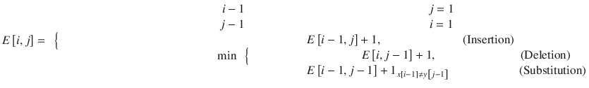
There are two base cases, capturing the edit distance of a prefix of x against an empty string or an empty string against a prefix of y, and then there are three cases for the recursion: one for insertion, where we move from ![]() to
to ![]() against
against ![]() ; one for deletion, where we move from
; one for deletion, where we move from ![]() to
to ![]() against
against ![]() ; and finally substitution, where we move from
; and finally substitution, where we move from ![]() against
against ![]() to
to ![]() against
against ![]() . The cost of this is 0 if
. The cost of this is 0 if ![]() and 1 if
and 1 if ![]() , which is captured by the indicator variable
, which is captured by the indicator variable ![]() .
.
This recursion is also readily translated into a dynamic programming algorithm. For test purposes, we can construct these two sequences:
x <- c("a", "b", "c")y <- c("a", "b", "b", "c")
where we can go from x to y by inserting one b, so the edit distance is 1.
Computing the recursion, using dynamic programming, could look like this:
n <- length(x)m <- length(y)E <- vector("numeric", length = (n + 1) * (m + 1))dim(E) <- c(n + 1, m + 1)for (i in 1:(n + 1))E[i, 1] <- i - 1for (j in 1:(m + 1))E[1, j] <- j - 1for (i in 2:(n + 1)) {for (j in 2:(m + 1)) {E[i, j] <- min(E[i - 1, j] + 1,E[i, j - 1] + 1,E[i - 1, j - 1] + (x[i - 1] != y[j - 1]))}}E## [,1] [,2] [,3] [,4] [,5]## [1,] 0 1 2 3 4## [2,] 1 0 1 2 3## [3,] 2 1 0 1 2## [4,] 3 2 1 1 1
The edit distance can be obtained by the bottom-right cell in this table:
E[n + 1, m + 1]## [1] 1
For both of these examples, it is straightforward to translate the recursions into dynamic programming algorithms, but the declarations of the problems—expressed in the recursions—are lost in the implementations, which are the loops where we fill out the tables.
We want to construct a domain-specific language that lets us specify a dynamic programming algorithm from a recursion and lets the language build the loops and computations for us. For example, we should be able to specify a recursion like this:
fib <- {F[n] <- 1 ? n <= 2F[n] <- F[n - 1] + F[n - 2]} %where% {n <- 1:10}
and have this expression build the Fibonacci table:
fib## [1] 1 1 2 3 5 8 13 21 34 55
In the recursion, we use the ? operator to specify the case in which a given rule should be used. You are probably familiar with ? used to get documentation for functions, but the R parser also considers it an infix operator and one with the lowest precedence at all—lower than even <- assignment. This, as it turns out, is convenient for this DSL. We specify the recursion cases as assignments, and by having an operator with lower precedence than an assignment, we will always have a ? call at the top level of the call expression if the rule has a condition associated with it.
Similarly to the Fibonacci recursion, we should be able to specify the edit-distance computation like this:
x <- c("a", "b", "c")y <- c("a", "b", "b", "c")edit <- {E[1,j] <- j - 1E[i,1] <- i - 1E[i,j] <- min(E[i - 1,j] + 1,E[i,j - 1] + 1,E[i - 1,j - 1] + (x[i - 1] != y[j - 1])) ? i > 1 && j > 1} %where% {i <- 1:(length(x) + 1)j <- 1:(length(y) + 1)}
and get the table computed:
edit## [,1] [,2] [,3] [,4] [,5]## [1,] 0 1 2 3 4## [2,] 1 0 1 2 3## [3,] 2 1 0 1 2## [4,] 3 2 1 1 1
Here, the first two cases are valid only when I or j is 1, respectively. We could specify this using ?, but I’m taking another approach. I use the index pattern on the left-hand side of the assignments to specify that an index variable should match a constant. This gives us semantics similar to the pattern matching in the previous chapter.
We could also have used this syntax for the Fibonacci recursion, like this:
{F[1] <- 1F[2] <- 1F[n] <- F[n - 1] + F[n - 2]} %where% {n <- 1:10}## [1] 1 1 2 3 5 8 13 21 34 55
For the semantics of evaluating the recursion, I will use the first rule where both index patterns and ? conditions are satisfied to compute a value. Since we always pick the first such expression, we don’t need to explicitly specify the conditions for the general case in the edit-distance specification, for example.
{E[1,j] <- j - 1E[i,1] <- i - 1E[i,j] <- min(E[i - 1,j] + 1,E[i,j - 1] + 1,E[i - 1,j - 1] + (x[i - 1] != y[j - 1]))} %where% {i <- 1:(length(x) + 1)j <- 1:(length(y) + 1)}## [,1] [,2] [,3] [,4] [,5]## [1,] 0 1 2 3 4## [2,] 1 0 1 2 3## [3,] 2 1 0 1 2## [4,] 3 2 1 1 1
Parsing Expressions
The examples give us an idea about what grammar we want for the language. We want it to look somewhat like this:
DYNPROG_EXPR ::= RECURSIONS '%where%' RANGESRECURSIONS ::= '{' PATTERN_ASSIGNMENTS '}'RANGES ::= '{' RANGES_ASSIGNMENTS '}'
At the top level, the language is implemented using the user-defined infix operator %where% . On the left-hand side of the operator, we want a specification of the recursion, and on the right-hand side, we want a specification of the ranges the algorithm should loop over. We can implement the operator like this:
`%where%` <- function(recursion, ranges) {parsed <- list(recursions = parse_recursion(rlang::enquo(recursion)),ranges = parse_ranges(rlang::enquo(ranges)))eval_dynprog(parsed)}
We simply parse the left-hand and right-hand sides and then call the function eval_ dynprog to run the dynamic programming algorithm and return the result.
The simplest aspect of the language is the specification of the ranges. Here, we define variables and associate them with sequences they should iterate over.
RANGES_ASSIGNMENTS ::= RANGES_ASSIGNMENT| RANGES_ASSIGNMENT ';' RANGES_ASSIGNMENTS
We want one or more assignments. Here, I’ve specified that we separate them by ;, but we will also accept newlines; we simply use what R uses to separate statements.
Assignments take the following form:
RANGES_ASSIGNMENT ::= RANGE_INDEX '<-' RANGE_EXPRESSIONI won’t break this down further, but just specify that RANGE_INDEX should be an R variable and RANGE_EXPRESSION an R expression that evaluates to a sequence.
In the %where% operator, we translate the ranges specification into a quosure, so we know in which scope to evaluate the values for the ranges, and then we process the result like this:
parse_ranges <- function(ranges) {ranges_expr <- rlang::get_expr(ranges)ranges_env <- rlang::get_env(ranges)stopifnot(ranges_expr[[1]] == "{")ranges_definitions <- ranges_expr[-1]n <- length(ranges_definitions)result <- vector("list", length = n)indices <- vector("character", length = n)for (i in seq_along(ranges_definitions)) {assignment <- ranges_definitions[[i]]stopifnot(assignment[[1]] == "<-")range_var <- as.character(assignment[[2]])range_value <- eval(assignment[[3]], ranges_env)indices[[i]] <- range_varresult[[i]] <- range_value}names(result) <- indicesresult}
First, we extract the expression and the environment of the quosure. We will process the former and use the latter to evaluate expressions. We expect the ranges to be inside curly braces, so we test this and extract the actual specifications. We iterate over them, expecting each to be an assignment, where we can get the index variable on the left-hand side and the expression for the actual ranges on the right-hand side. We evaluate the expressions, in the quosure scope, and build a list as the parse result. This list will contain one item per range expression. The name of the item will be the iterator value, and the value will be the result of evaluating the corresponding expression.
parse_ranges(rlang::quo({n <- 1:10}))## $n## [1] 1 2 3 4 5 6 7 8 9 10parse_ranges(rlang::quo({i <- 1:(length(x) + 1)j <- 1:(length(y) + 1)}))## $i## [1] 1 2 3 4#### $j## [1] 1 2 3 4 5
The recursion specifications are slightly more complicated.
PATTERN_ASSIGNMENTS ::= PATTERN_ASSIGNMENT| PATTERN_ASSIGNMENT ';' PATTERN_ASSIGNMENTS
where
PATTERN_ASSIGNMENT ::= PATTERN '<-' RECURSION| PATTERN '<-' RECURSION '?' CONDITIONPATTERN ::= TABLE '[' INDICES ']'
We won’t break the grammar down further than this. Here TABLE is a variable, INDICES is a comma-separated sequence of variables or expressions, and both RECURSION and CONDITION are R expressions.
With this grammar, we need to extract three different pieces of information: the index patterns, so we can match against that; the ? conditions, such that we can check those; and finally the actual recursions. The parser doesn’t have to be much more complicated than for the ranges, though, as long as we just collect these three properties of each recursive case and put them in lists.
parse_recursion <- function(recursion) {recursion_expr <- rlang::get_expr(recursion)recursion_env <- rlang::get_env(recursion)stopifnot(recursion_expr[[1]] == "{")recursion_cases <- recursion_expr[-1]n <- length(recursion_cases)patterns <- vector("list", length = n)conditions <- vector("list", length = n)recursions <- vector("list", length = n)for (i in seq_along(recursion_cases)) {case <- recursion_cases[[i]]condition <- TRUEstopifnot(rlang::is_call(case))if (case[[1]] == "?") {# NB: The order matters here!condition <- case[[3]]case <- case[[2]]}stopifnot(case[[1]] == "<-")pattern <- case[[2]]recursion <- case[[3]]patterns[[i]] <- patternrecursions[[i]] <- recursionconditions[[i]] <- condition}list(recursion_env = recursion_env,patterns = patterns,conditions = conditions,recursions = recursions)}
The function is not substantially different from the parser for the ranges. We extract the quosure environment and the expression, check that it is a call to curly braces, and then loop through the cases.
If a case is a call to ?, we know it has a condition. Since ? has the lowest precedence of all operators, it will be the top-level call if a condition exists—unless, at least, users get cute with parentheses, but then they get what they deserve. As a default condition, we use TRUE. This way, we don’t have to deal with special cases when there is no ? condition specified; but if there is, we replace TRUE with the expression. Otherwise, we just collect all the information for each recursive case.
We do not evaluate the recursions in the parser, so we do not use the quosure environment in the parser. Instead, we return it together with the parsed information. We will need it later when we evaluate the recursion expressions.
We can test the parser on the Fibonacci recursion to see how it behaves.
parse_recursion(rlang::quo({F[n] <- n * F[n - 1] ? n > 1F[n] <- 1 ? n <= 1}))## $recursion_env## <environment: R_GlobalEnv>#### $patterns## $patterns[[1]]## F[n]#### $patterns[[2]]## F[n]###### $conditions## $conditions[[1]]## n > 1#### $conditions[[2]]## n <= 1###### $recursions## $recursions[[1]]## n * F[n - 1]#### $recursions[[2]]## [1] 1
Similarly, we can use it to parse the edit-distance recursions.
parse_recursion(rlang::quo({E[1,j] <- j - 1E[i,1] <- i - 1E[i,j] <- min(E[i - 1,j] + 1,E[i,j - 1] + 1,E[i - 1,j - 1] + (x[i - 1] != y[j - 1])) ? i > 1 && j > 1}))## $recursion_env## <environment: R_GlobalEnv>#### $patterns## $patterns[[1]]## E[1, j]#### $patterns[[2]]## E[i, 1]#### $patterns[[3]]## E[i, j]###### $conditions## $conditions[[1]]## [1] TRUE#### $conditions[[2]]## [1] TRUE#### $conditions[[3]]## i > 1 && j > 1###### $recursions## $recursions[[1]]## j - 1#### $recursions[[2]]## i - 1#### $recursions[[3]]## min(E[i - 1, j] + 1, E[i, j - 1] + 1, E[i - 1, j - 1] + (x[i -## 1] != y[j - 1]))
Evaluating Expressions
To evaluate a dynamic programming expression, we need to iterate over all the ranges, compute the first value associated with satisfied conditions and patterns, and put the result in the dynamic programming table. We could construct expressions with nested loops for the ranges to do this, but there is a simpler way. We can construct all combinations of ranges using the expression do.call(expand.grid, ranges). For the Fibonacci example, we get this:
ranges <- parse_ranges(rlang::quo({n <- 1:10}))head(do.call(expand.grid, ranges))## n## 1 1## 2 2## 3 3## 4 4## 5 5## 6 6
Except that we have a name associated with the range, this is just the input. For the edit-distance example, we see the full use of this expression here:
ranges <- parse_ranges(rlang::quo({i <- 1:(length(x) + 1)j <- 1:(length(y) + 1)}))head(do.call(expand.grid, ranges))## i j## 1 1 1## 2 2 1## 3 3 1## 4 4 1## 5 1 2## 6 2 2
Here, we get all combinations of i and j from the ranges. Instead of constructing expressions with nested loops, we can iterate through the rows of the table we get from this invocation. If we extract a row, we get a vector with named range indices.
edit_ranges <- do.call(expand.grid, ranges)edit_ranges[1,]## i j## 1 1 1edit_ranges[2,]## i j## 2 2 1
Using the with function, we can exploit this to create an environment where range indices are bound to values, and it is in precisely such environments we want to evaluate the recursions.
with(edit_ranges[3,],cat(i, j, " "))## 3 1
Looping over the rows in a table we create this way will be the core of our algorithm. Before we get to implementing this, however, we need to construct the expressions to insert into the body of the loop.
We start with creating code for testing patterns against range-index variables. Here, we will keep the syntax simpler than the pattern matching from the previous chapter. We assume that the indices in the left-hand side of recursions consist of index variables or constants, and we build a test that simply compares the index-variable names, which we get from the ranges parser, against the values in the recursion specification. We can construct the function as simply as this:
make_pattern_match <- function(pattern, range_vars) {matches <- vector("list", length = length(range_vars))stopifnot(pattern[[1]] == "[")for (i in seq_along(matches)) {matches[[i]] <- call("==",pattern[[i + 2]],range_vars[[i]])}rlang::expr(all(!!! matches))}
We construct a list of == comparisons between the index patterns used in the specification and the values the range indices can iterate over. For the latter, we first need to translate strings into symbols, so we are sure to compare the values of pattern variables and not check that constants match the name of the variables. We do not perform that conversion inside this function; we will expect that the caller has already done this. The reason that we use index i + 2 for the patterns is that patterns are in the form of a call to the [ operator, so index 1 is the [ symbol and index 2 is the table name. The indices follow after those two argument-elements.
A couple of examples should illustrate how the pattern-matching predicates are constructed.
make_pattern_match(rlang::expr(F[1]), list(as.symbol("n")))## all(1 == n)make_pattern_match(rlang::expr(F[n]), list(as.symbol("n")))## all(n == n)make_pattern_match(rlang::expr(E[1,j]),list(as.symbol("i"), as.symbol("j")))## all(1 == i, j == j)
We test all range variables, even when they are completely free to take any values. When they are, we simply check that they equal themselves, which they will always do unless they are NA—and if they are, there isn’t anything useful we can do about them anyway. Creating the test this way makes the code for testing patterns simpler, and testing that variables equal themselves does not change the result the conditions end up with.
We map this expression construction over all the patterns to get test-code for all recursive cases.
make_pattern_tests <- function(patterns, range_vars) {tests <- vector("list", length = length(patterns))for (i in seq_along(tests)) {tests[[i]] <- make_pattern_match(patterns[[i]],range_vars)}tests}
Given these Fibonacci parser results:
fib_ranges <- parse_ranges(rlang::quo({n <- 1:10}))fib_recursions <- parse_recursion(rlang::quo({F[n] <- F[n - 1] + F[n - 2] ? n > 2F[n] <- 1 ? n <= 2}))
we can construct the pattern tests for all cases like this:
make_pattern_tests(fib_recursions$patterns,Map(as.symbol, names(fib_ranges)))## [[1]]## all(n == n)#### [[2]]## all(n == n)
We want to know if both pattern and ? condition match before we evaluate an expression, so we combine the two lists. We simply construct a new list where we combine the pattern matching with the ? conditions using &&.
make_condition_checks <- function(ranges,patterns,conditions,recursions) {test_conditions <- make_pattern_tests(patterns,Map(as.symbol, names(ranges)))for (i in seq_along(conditions)) {test_conditions[[i]] <- rlang::call2("&&", test_conditions[[i]], conditions[[i]])}test_conditions}
To verify that this works as intended, we can, again, use the Fibonacci recursions.
fib_ranges <- parse_ranges(rlang::quo({n <- 1:10}))fib_recursions <- parse_recursion(rlang::quo({F[n] <- F[n - 1] + F[n - 2] ? n > 2F[n] <- 1 ? n <= 2}))make_condition_checks(fib_ranges,fib_recursions$patterns,fib_recursions$conditions,fib_recursions$recursions)## [[1]]## all(n == n) && n > 2#### [[2]]## all(n == n) && n <= 2
So, the status is now that we have all the test conditions. We can take these test conditions, combine them with the expressions for evaluating the recursions, and construct a sequence of if-else expressions. If we construct an if call with two arguments, this is interpreted as the test condition and the value to compute when the test is true. If we construct a call with three arguments, the third is considered the else part of the statement. The simplest way to construct a sequence of if-else statements is, therefore, to start from the end of the list. We can translate the last case into an if statement without an else part—or we can make an else part that throws an error if we prefer. We can then iterate through the cases, at each case constructing a new if expression that takes the previous case as the else part. This idea can be implemented like this:
make_recursion_case <- function(test_expr,value_expr,continue) {if (rlang::is_null(continue)) {rlang::call2("if", test_expr, value_expr)} else {rlang::call2("if", test_expr, value_expr, continue)}}make_update_expr <- function(ranges,patterns,conditions,recursions) {conditions <- make_condition_checks(ranges,patterns,conditions,recursions)continue <- NULLfor (i in rev(seq_along(conditions))) {continue <- make_recursion_case(conditions[[i]], recursions[[i]], continue)}continue}
For the Fibonacci recursion, the result is this expression:
make_update_expr(fib_ranges,fib_recursions$patterns,fib_recursions$conditions,fib_recursions$recursions)## if (all(n == n) && n > 2) F[n - 1] + F[n - 2] else if (all(n ==## n) && n <= 2) 1
What remains to be done is to evaluate this expression for each combination of range indices. To do this, we create the table using the do.call expression we saw earlier, loop over all table rows, and insert the update expression inside the body of the loop. A function for creating the entire loop function looks like this1:
make_loop_expr <- function(tbl_name, update_expr) {rlang::expr({combs <- do.call(expand.grid, ranges)rlang::UQ(tbl_name) <- vector("numeric",length = nrow(combs))dim(rlang::UQ(tbl_name)) <- Map(length, ranges)for (row in seq_along(rlang::UQ(tbl_name))) {rlang::UQ(tbl_name)[row] <- with(combs[row, , drop = FALSE], {rlang::UQ(update_expr)})}rlang::UQ(tbl_name)})}
In addition to the update_expr, the code needs to know the table name. This is because the update_expr will be referring to the table in the recursive cases. The table name is easy to get from the patterns, though.
get_table_name <- function(patterns) {p <- patterns[[1]]stopifnot(p[[1]] == "[")p[[2]]}get_table_name(fib_recursions$patterns)## F
The loop, expanded with expressions from the Fibonacci recursion, looks like this:
make_loop_expr(get_table_name(fib_recursions$patterns),make_update_expr(fib_ranges,fib_recursions$patterns,fib_recursions$conditions,fib_recursions$recursions))## {## combs <- do.call(expand.grid, ranges)## F <- vector("numeric", length = nrow(combs))## dim(F) <- Map(length, ranges)## for (row in seq_along(F)) {## F[row] <- with(combs[row, , drop = FALSE], {## if (all(n == n) && n > 2)## F[n - 1] + F[n - 2]## else if (all(n == n) && n <= 2)## 1## })## }## F## }
For the edit-distance recursion , we get the following:
edit_ranges <- parse_ranges(rlang::quo({i <- 1:(length(x) + 1)j <- 1:(length(y) + 1)}))edit_recursions <- parse_recursion(rlang::quo({E[1,j] <- j - 1E[i,1] <- i - 1E[i,j] <- min(E[i - 1,j] + 1,E[i,j - 1] + 1,E[i - 1,j - 1] + (x[i - 1] != y[j - 1]))}))make_loop_expr(get_table_name(edit_recursions$patterns),make_update_expr(edit_ranges,edit_recursions$patterns,edit_recursions$conditions,edit_recursions$recursions))## {## combs <- do.call(expand.grid, ranges)## E <- vector("numeric", length = nrow(combs))## dim(E) <- Map(length, ranges)## for (row in seq_along(E)) {## E[row] <- with(combs[row, , drop = FALSE], {## if (all(1 == i, j == j) && TRUE)## j - 1## else if (all(i == i, 1 == j) && TRUE)## i - 1## else if (all(i == i, j == j) && TRUE)## min(E[i - 1, j] + 1, E[i, j - 1] + 1, E[i - 1,## j - 1] + (x[i - 1] != y[j - 1]))## })## }## E## }
All that remains now is to evaluate this loop expression, and the only trick to this is to make sure we evaluate it in the right environment. The with statement inside the loop ensures that we over-scope the expression with the relevant index variables, so we do not have to worry about the ranges and range indices. The expressions we evaluate in the update expression, however, should be evaluated in the scope where we define the expression, which we captured in the quosures when we parsed the expressions. Ideally, we would just evaluate the loop in this quosure environment, but the loop expression needs to know about the ranges, so we need to put those in the scope as well. One way to do this is to put a local function-call environment between the quosure scope and the loop and evaluate the expression this way:
eval_recursion <- function(ranges, recursions) {loop <- make_loop_expr(get_table_name(recursions$patterns),make_update_expr(ranges,recursions$patterns,recursions$conditions,recursions$recursions))eval_env <- rlang::env_clone(environment(), # this function environmentrecursions$recursion_env # quosure environment)eval(loop, envir = eval_env)}
For the Fibonacci expressions, we get the following:
eval_recursion(fib_ranges, fib_recursions)## [1] 1 1 2 3 5 8 13 21 34 55
The %where% operator, as we saw earlier in this chapter, simply parses the ranges and recursions and then evaluates the result in a function called eval_dynprog. This function does nothing more than call the eval_recursion function we just wrote.
eval_dynprog <- function(dynprog) {eval_recursion(dynprog$ranges, dynprog$recursions)}
Providing the parsed pieces directly to the eval_dynprog function, instead of going through %where%, we see that this is indeed what is happening.
eval_dynprog(list(ranges = fib_ranges,recursions = fib_recursions))## [1] 1 1 2 3 5 8 13 21 34 55eval_dynprog(list(ranges = edit_ranges,recursions = edit_recursions))## [,1] [,2] [,3] [,4] [,5]## [1,] 0 1 2 3 4## [2,] 1 0 1 2 3## [3,] 2 1 0 1 2## [4,] 3 2 1 1 1
Fixing the Evaluation Environment
The solution so far works, but there is one slightly unsatisfactory aspect of the solution. When we evaluate the loop, we place an environment between the quosure environment and the expression we evaluate, and this environment contains several local variables that can potentially conflict with variables in the quosure scope.
We can avoid this and make sure that we only over-scope with the range-index variables and nothing else, but we will then have to take a slightly different approach. Instead of constructing the loop as an expression and then evaluating it in the function-plus quosure-scope, we loop over the range-index combinations immediately. In the body of the loop, we construct and evaluate the update expressions.2
The alternative solution is listed next. As in the previous solution, we get the name of the dynamic-programming table first, and we construct the update expression. This time, though, we also get hold of the table name as a string. We need this to access the name in the evaluation environment, which we construct as an empty environment with the quosure environment as the parent. That way, we can modify the evaluation environment without affecting the quosure environment, but we still have access to all variables we can get from there.
We don’t need any meta-programming to construct the table. We can get its size and dimensions from the ranges. We need to put it in the evaluation environment for the update expressions to see, though, and we do that using the [[ operator on environments. After constructing the table and putting it in the evaluation environment, we loop through all the range-index combinations as before.
We want to over-scope the update expression with the index variables when we compute the recursion values, so we need to evaluate the expression in an environment that contains combs[row,]. We cannot evaluate the actual assignment if we use this row as the second argument to eval, however. R considers the second argument to eval the environment where expressions are evaluated, and an assignment in an environment that is really a list will not work. You will not get an error, but you will not assign to any variable either. So, we need to split the evaluation of the recursion and the assignment to the table in two. We evaluate the recursion expression in an environment where combs[row,] over-scopes the evaluation environment, and we evaluate the assignment in the evaluation environment without any other over-scoping.
You might think that once we have the value to insert in the table, we could just update the table, and we wouldn’t have to construct an assignment expression to achieve this. It is not that simple, however. R tries very hard to make data immutable, and if we assign to an element in a table that is referenced from two different places, R will copy the table, update only one of the copies, and set the modified copy in the environment where we did the assignment, leaving the original in the other scope. To update the table, such that the recursion expressions can use it, we need to do the update in the evaluation environment (or alternatively, update the table and then assign the copy into the evaluation environment).
The alternative evaluation function thus looks like this:
eval_recursion <- function(ranges, recursions) {tbl_name <- get_table_name(recursions$patterns)tbl_name_string <- as.character(tbl_name)update_expr <- make_update_expr(ranges,recursions$patterns,recursions$conditions,recursions$recursions)eval_env <- rlang::child_env(recursionsxs$recursion_env)combs <- do.call(expand.grid, ranges)tbl <- vector("numeric", length = nrow(combs))dim(tbl) <- Map(length, ranges)eval_env[[tbl_name_string]] <- tblfor (row in seq_along(tbl)) {val <- eval(rlang::expr(rlang::UQ(update_expr)),combs[row, , drop = FALSE],eval_env)eval(rlang::expr(rlang::UQ(tbl_name)[rlang::UQ(row)]<- rlang::UQ(val)), eval_env)}eval_env[[tbl_name_string]]}
It behaves exactly like the previous one, though.
eval_dynprog(list(ranges = fib_ranges,recursions = fib_recursions))## [1] 1 1 2 3 5 8 13 21 34 55eval_dynprog(list(ranges = edit_ranges,recursions = edit_recursions))## [,1] [,2] [,3] [,4] [,5]## [1,] 0 1 2 3 4## [2,] 1 0 1 2 3## [3,] 2 1 0 1 2## [4,] 3 2 1 1 1
At least, unless your recursions referenced variables that would be over-scoped by local variables in the previous version.
Footnotes
1 The drop=FALSE in the row subscript ensures that we get a row with a named variable even when there is only one.
2 Depending on your taste, you might prefer this solution over the previous just because we keep evaluation of generated code to a minimum. The new solution involves generating and evaluating more expressions, though, and some hacks to update the table in the scope where we evaluate recursions, so the first solution has some merits over the second.