Scopes and Environments

R evaluates an expression in a scope that determines which value any given variable refers to. In the standard evaluation, R uses what is known as lexical scope. This essentially means that variables in an expression are referring to the variables defined in the blocks around the expression. If you write an expression at the outermost level of an R script, or in the global environment , then variable names in the expression refer to global variables. An expression inside a function, on the other hand, is evaluated in the scope of a function execution, which means that variable symbols refer to local variables or function parameters if they are defined; only if they are not defined do they refer to global variables. A function defined inside another function will have a nested scope—variables in an expression there will first be searched for in the innermost function, then the surrounding function, and only if they are not found either place, in the global environment.

Consider this abstract example:

x <- 1
f <- function(y) {
  z <- 3
  function() x + y + z
}
g <- f(2)
h <- f(3)
g()

## [1] 6

h()

## [1] 7

In the example, we define four variables in the global environment, x, f, g, and h. In the function f we have one formal parameter, y, and one local variable, z. Whenever we call f, a scope where y exists is created, and the first statement in the function call adds z to this scope. The function returns another function, a closure, that contains an expression that refers to variables x, y, and z. If we call this function, which we do when we call functions g and h that are the results of two separate calls to f, we will evaluate this expression. When R evaluates the expression, it needs to find the three variables. They are neither formal arguments nor local variables in the functions we call (g and h), but since the functions were created inside calls to f, they can see y and z in their surrounding scope. Both can find x in the global environment. Since g and h are the results of separate calls to f, the surrounding scope of calls to them are different instances of local scopes of f.

Scopes are implemented through environments, and even though the rules that guide environments and evaluation are straightforward, you have to be careful if you start manipulating them. You can think of environments as tables that map variables to values. Also, all environments have a parent environment, an enclosing scope, that R will search in if a variable is not found when it searches the first environment. Environments thus have a tree structure that usually follows nested scopes, and that ends in a root in the empty environment. Packages you load are put on top of this environment, and on top of all loaded environments, we have the global environment—which is why you can find variables defined in packages if you search in the global environment.

Strictly speaking, there are a few other details on how packages and environments interact that I do not include in this view on environments, but they are not important for the discussion here. If you are interested, you can find these details in my other book, Meta-programming in R (Mailund, 2017c). For this book, we will simply assume that everything we define at the global level or any package is found in the global environment and consider this the root of the environment tree.

When we define new functions, we do not create new environments, but we do associate the functions with one—the environment in which we define the function. When we defined function f in the previous example, it got associated with the global environment, because that is where we defined it. We can get the environment a function is associated with using the environment function.

environment(f)

## <environment: R_GlobalEnv>

Since f is defined at the global level, its environment is the global environment. When we make a function call, we create a new environment called the execution environment. This environment is where we store parameters and local variables. The environment associated with the function will be the parent environment for this execution environment. When we call function f, we thus create an environment where we get a mapping from y and z to their values and with a parent environment that is the global environment, in which we can find the variable x. Inside the call to f, we create a new (anonymous) function and return it. This function will also have an environment associated with it, but this time it is the local environment we created when we called f. Thus, the environments associated with g and h are two different environments as they are the result of two different calls to f.

environment(g)

## <environment: 0x7fdd80b25f08>

environment(h)

## <environment: 0x7fdd80a7f468>

Functions defined inside other functions thus carry along with them the environments that were created when the surrounding function was called, and if we return them from the surrounding function, they still carry this enclosing scope along with them. Since they remember the local variable and parameters from the enclosing scope, we call such functions closures.

In Figure 7-1, I have drawn a simplified graph that shows which environments exist and how they are wired together in the example at the point where we call function g. I show environments with a gray background, variables as circles with pointers to the values the variables refer to, and functions as the three components that define a function: the formal parameters, the function body, and the enclosing scope—the environment associated with the function.

The enclosing environment for function f is the global environment, while the enclosing scopes of g and h are the two different instances of calls to f. These instance or execution environments have the global environment as their parents since that is the enclosing scope of f. Because they are two different instances of f, the variables in them can point to different values, as we see for the variable y. For function g, y points to 3, while for function h, y points to 2. In a call to function g, we create a local environment for the function call—shown at the bottom right in the figure. We do not have any local variables in g, so this environment does not contain any variables, but it has a parent that is the f instance where we created g.

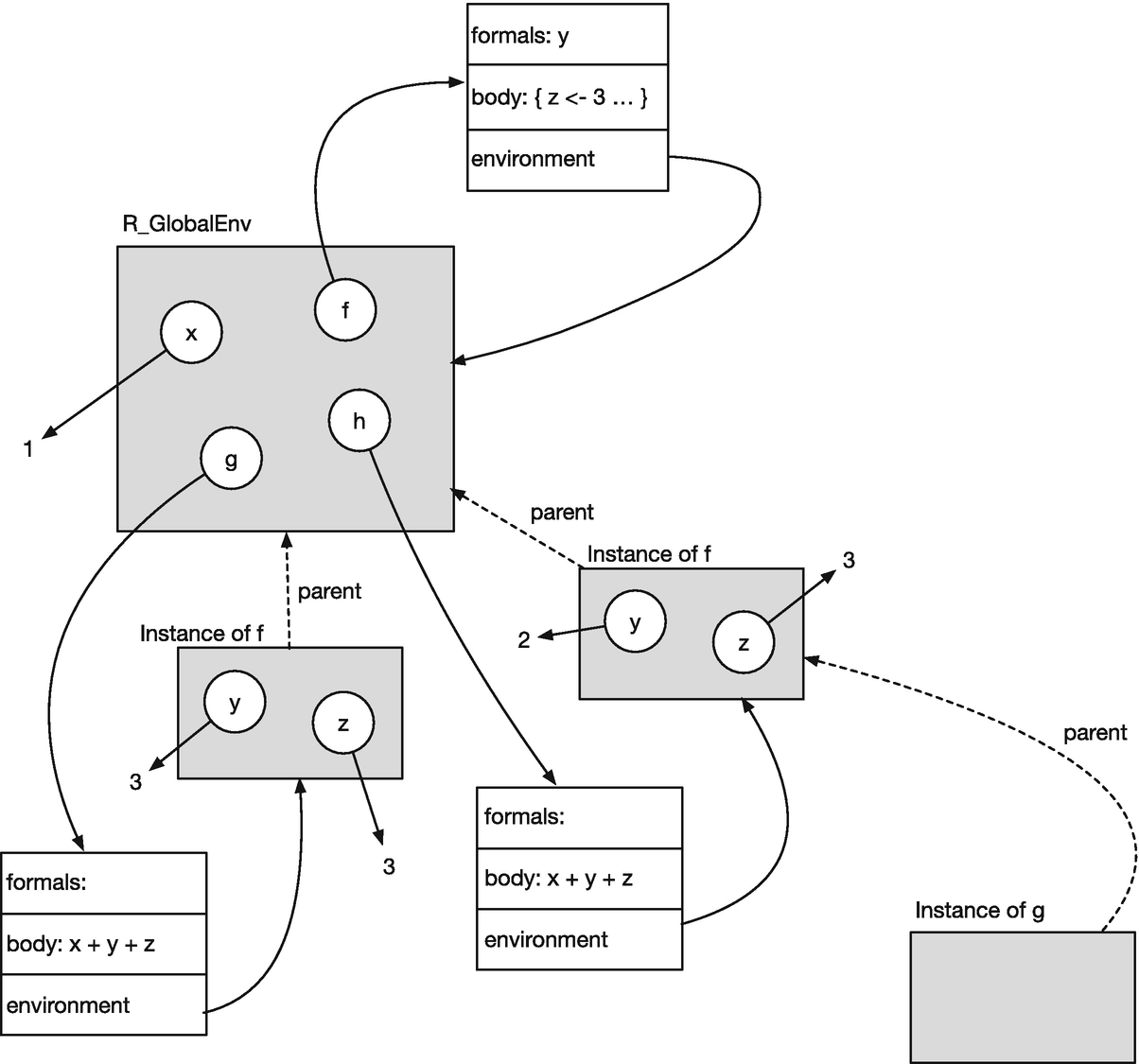
Figure 7-1 Environment graph when calling g

When we evaluate the expression x + y + z inside the call to g, we need to map variables to values. The search will start in the local environment and then progress up the parent links until it finds a matching variable. For variables y and z we find values in the parent of the g call, the instance of the f call that created g. For x we find the value in the grandparent, the global environment.

The rule for evaluating expressions is always the same: we look for variables by searching in environments, starting with the immediate environment where we evaluate the expression and search along the chain of parent environments. We check each environment in the chain in turn until we find the variable we are looking for. We get the standard evaluation rules of lexical scoping because functions get associated with the environment where they are created and since this environment is set as the parent environment of execution environments. The only trick to understanding how expressions are evaluated in R is to understand which environments are used. For the body of functions, it is as simple as I have just explained, but for function parameters, there are a few more rules to consider.

Default Parameters, Lazy Evaluation, and Promises

When you pass primitive values such as numbers to a function parameter, there is nothing we need to evaluate, so there are no complications. This is why we didn’t have to worry about the environment of the arguments in the previous example. If we pass expressions along as parameters, however, we need to know how they should be evaluated.

Most of the time, R behaves as if expressions are evaluated before a function is called, but this not what happens. If we passed values to functions rather than expressions, we would not be able to get the expressions using substitute as we have done in previous chapters. When we call a function in R, the parameters will refer to unevaluated expressions; such expressions are known as promises. Promises are evaluated the first time we use a parameter variable but not before—an approach to parameter evaluation known as lazy evaluation. If we never refer to an argument, the corresponding expression will never be evaluated, so we can write code such as this without raising exceptions:

f <- function(x, y) x
f(2, stop("error!"))

## [1] 2

We never refer to the parameter y inside the body of f, so we never evaluate it. Consequently, we never call stop to raise the error.

So, since parameters can contain expressions, we need a rule for how to evaluate them. Here, there is a difference between default parameters, defined when the function is created, and parameters provided when the function is called. The former is evaluated in the local scopes of function calls, while the latter is evaluated in the environment where the function is called.

Consider this function:

f <- function(y, z = 2 * y) y + z

The function takes two parameters, y and z.

f(2, 1)

## [1] 3

But if we only provide y, then z will be set to 2 * y.

f(2)

## [1] 6

When we evaluate the promise that z points to when the function is called—we do this in the expression where we use the variable—the promise expression is evaluated. This means that R needs to find the variable y. If we try to evaluate the expression 2 * y in the scope where the function is defined—the global environment—then we would get an error, as there is no y variable defined there. The semantics of default parameters could be such that we evaluated them in the scope where we define a function. If so, we wouldn’t be able to make default parameters depend on other parameters, which is what we want here—we want z to depend on y if we do not explicitly provide a value to it. The actual semantics is that the promise is evaluated in the function-call environment. When we call f, before we evaluate the y + z expression, the situation is therefore as shown in Figure 7-2. Here, I have drawn the promise for z as the expression passed along as the function argument together with the environment in which it should be evaluated.

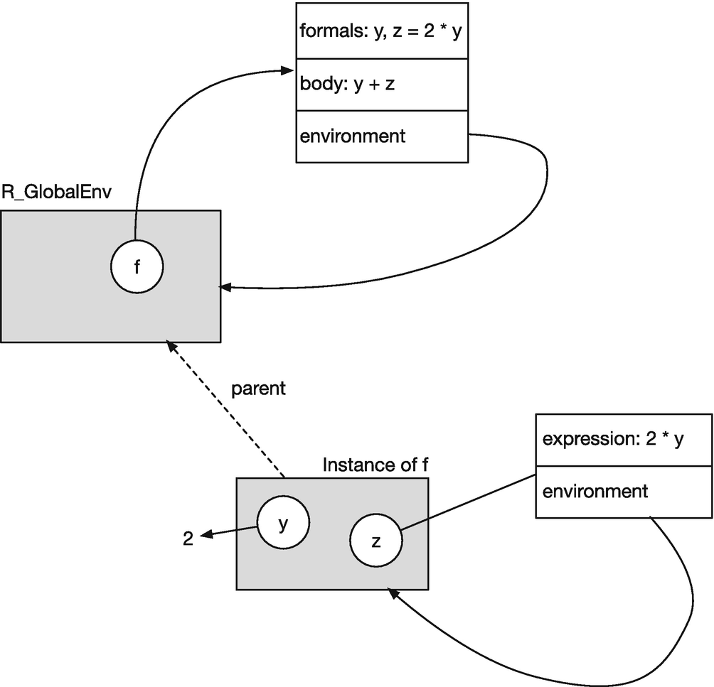
Figure 7-2 Default parameter promise

When we call f with a parameter that is an expression, we do not want to evaluate this expression in function-call scope. Consider this:

y <- 2
f(2 * y)

## [1] 12

The intent is to call f with 2 * y, which should be 4 since y is 2. If we tried to evaluate it inside the function call, however, we would have a circular dependency. Inside the function call, y is a variable, and if it points to 2 * y, we cannot evaluate the expression without knowing what y is, which we cannot know until we have evaluated the expression, which we cannot because we do not know what y is….

When we call a function with an expression as an argument, the corresponding promise will be evaluated in the environment where we call the function, so before we evaluate y + z inside f, the situation is as shown in Figure 7-3. Inside the environment of the function call, both y and z refer to promises, but these promises are associated with different environments. To evaluate the expression y + z, we need to evaluate both promises. To get the value for y, we need to evaluate 2 * y in the global scope, which gives us 4, and to get the value for z we need to evaluate 2 * y in the local scope, which gives us 8.

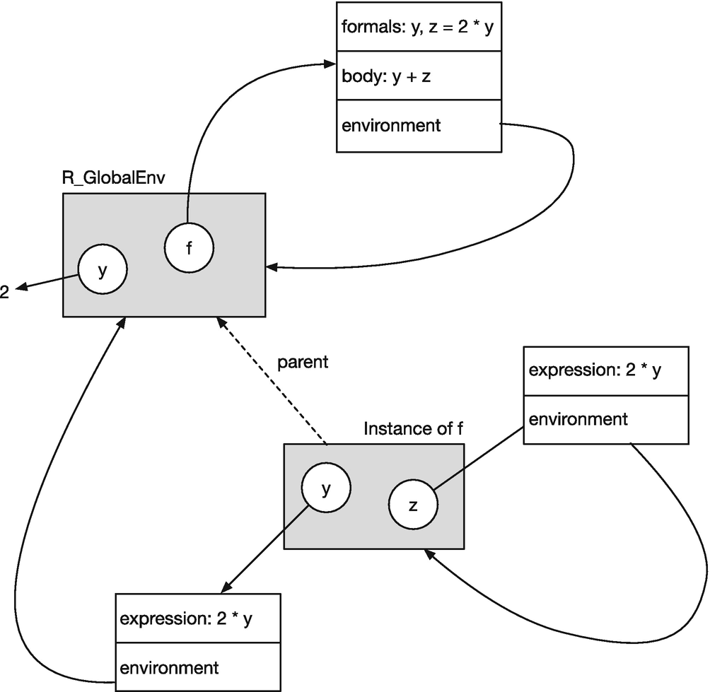
Figure 7-3 Calling f with an expression for y

At the risk of taking the example a step too far, let’s consider the situation where we call f from another function.

g <- function(x) f(2 * x)
g(2 * y)

## [1] 24

Before we evaluate the expression y + z inside function f, the state of the environment graph is as shown in Figure 7-4. It takes a little effort to see what happens when we want to evaluate y + z, but doing this exercise will go a long way toward understanding environments.

Figure 7-4 Calling g with an expression for x that depend on variable y

We have not yet evaluated the promises y and z. Since z depends on y, we need to evaluate y first. To do this, we need to evaluate the expression 2 * x in the scope of the call to g. Here, we need to evaluate x, which is another promise: the expression 2 * y that should be evaluated in the global scope (where y refers to a different variable than the local variable inside the f instance). In the global scope, y refers to the value 2, so we can evaluate 2 * y directly and get the value 4. This value then replaces the promise in the scope of the call to g. Once we have evaluated a promise, the variable refers to the value and no longer the expression. This now means that we can evaluate 2 * x in the scope of the g call to get 8. So now y in the call to f refers to 8. This means we can evaluate 2 * y to get 16, which we assign the variable z. Finally, we can evaluate y + z to get 8 + 16 = 24.

To summarize this section, parameters we pass to functions, if they are not primitive values, are considered expressions that must be evaluated at some point. Associated with the expressions, we have a scope in which to evaluate the them. There is one more caveat, though, which I hinted to in the previous example: parameters are considered expressions only until the first time we evaluate them. After that, they are the result of this evaluation.

There are pros and cons with these semantics—though predominantly cons. We can avoid computing values we do not need because promises are not evaluated until we refer to the variable that holds them. Moreover, we can make default parameters that depend on some computation inside a function call as long as we do those computations before we use the variable that needs them. For example, we can define a default parameter in terms of a variable we set inside a function.

h <- function(x, y = 2 * w) {
  w <- 2
  x + y
}
h(1)

## [1] 5

However, this will fail if we refer to the promise that needs the variable before we compute it.

h <- function(x, y = 2 * w) {
  res <- x + y
  w <- 2
  res
}
h(1)

## Error in h(1): object 'w' not found

We have to be careful if a promise depends on a variable that we update during a computation. Note that a promise is evaluated only once; after the evaluation, the variable that used to hold it now holds the result of the evaluation and no longer the promise expression. If we change variables that occurred in the promise, we do not update the value that the variable now holds.

h <- function(x, y = 2 * w) {
  w <- 1
  res <- x + y
  w <- 2
  res
}
h(1)

## [1] 3

The promises held by default parameters do not usually cause problems. It is simple to follow which local variables will change in the function and at what point the promise will be evaluated. Lazy evaluation of arguments, however, is a common source of problems when combined with closures. Consider this function:

make_adder <- function(n) function(m) n + m

This returns a closure that will add n to its argument, m. We can use it like this:

add_1 <- make_adder(1)
add_2 <- make_adder(2)
add_1(1)

## [1] 2

add_2(1)

## [1] 3

No problems here, but now consider this:

adders <- vector("list", 3)
for (i in 1:3) adders[[i]] <- make_adder(i)

The intent here is to create three adder functions that add 1, 2, and 3, respectively, to their argument. When we call the first function, though, we get an unpleasant surprise.

adders[[1]](1)

## [1] 4

The expression n + m inside the closure is not evaluated until we call it. Before we evaluate the body in the adders[[1]](1) call, the environment graph looks like Figure 7-5. All three adders are closures that refer to different instances of make_adders, but all these instances have n refer to a promise that is the expression i. The variable i is found in the global environment and not in the closure environment. After we have created all three closures, i refers to the number 3. To evaluate n + m inside the adder, we must first evaluate the promise that n refers to. We search for n and find it in the parent environment of the function call (the closure environment) where n refers to i that should be evaluated in the global environment. We evaluate it and now n refers to 3, as shown in Figure 7-6. This is why the result of calling adders[[1]] with m set to 1 returns 4 and not 2.

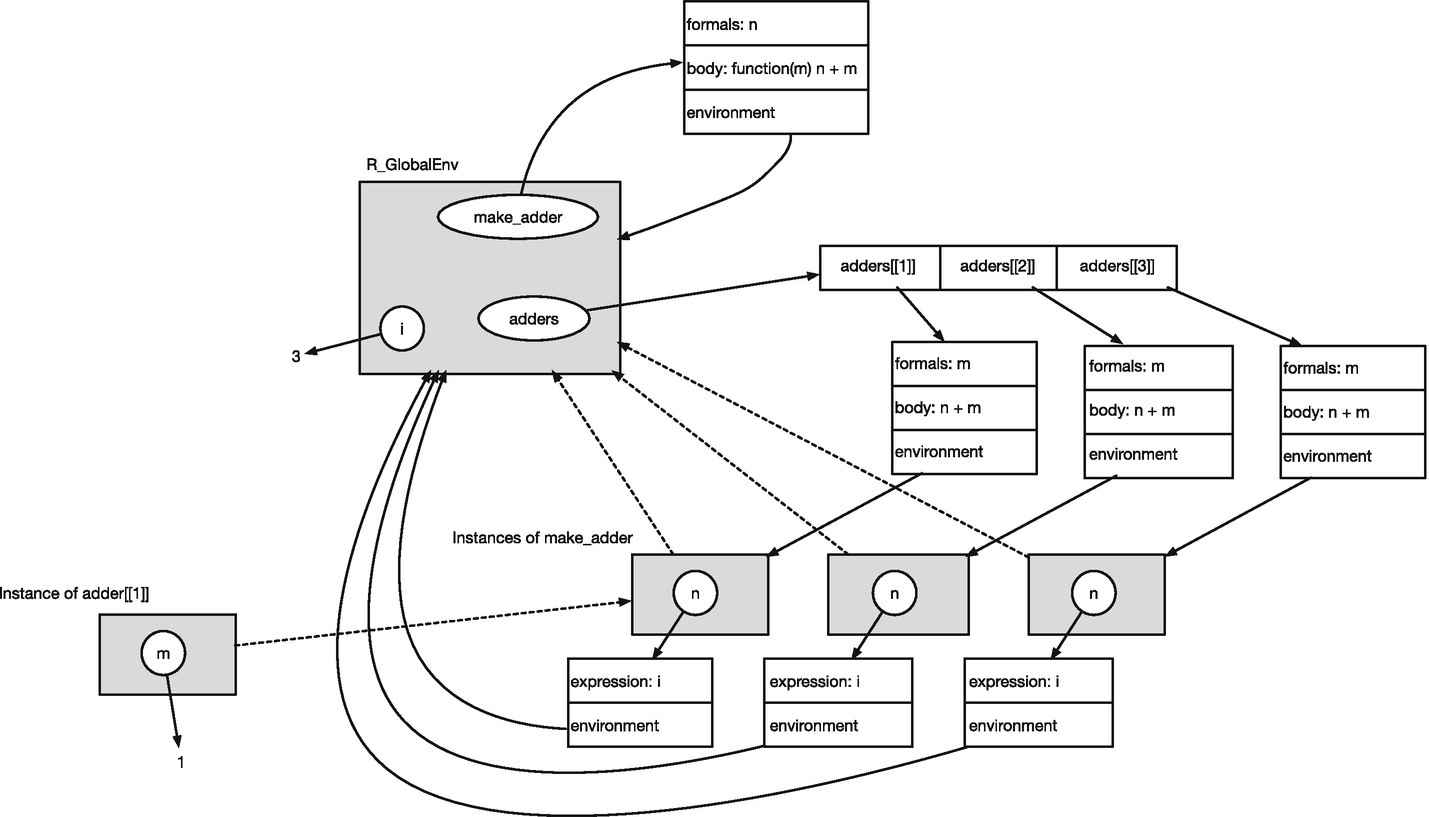
Figure 7-5 Adders before evaluating the body of the adders[[1]](1) call

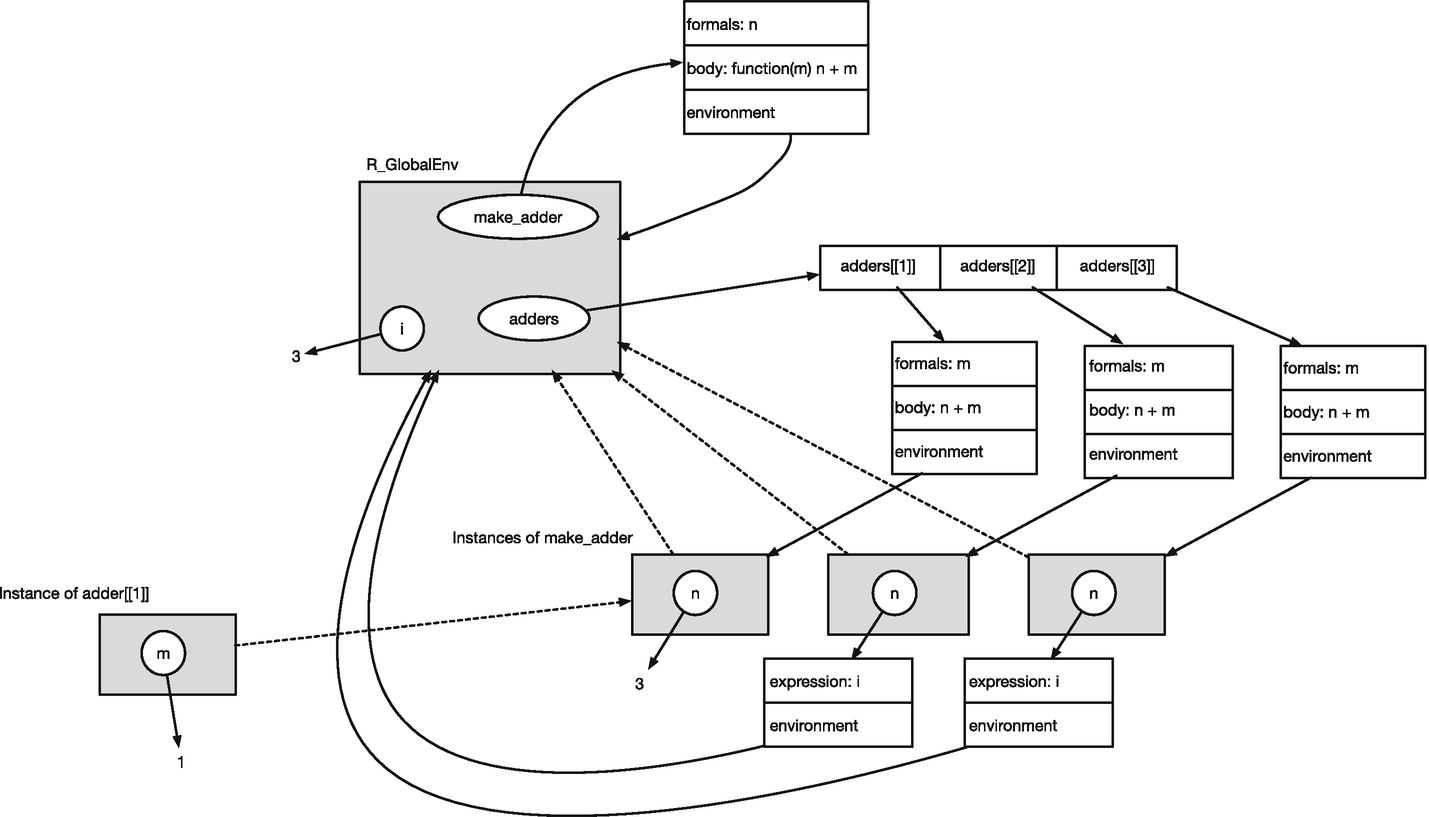
Figure 7-6 Adders after evaluating the n promise in adders[[1]]

After we have called this closure, the variable n no longer refers to a promise but to the value 3, so changing i at this point will not affect the closure.

i <- 1
adders[[1]](1)

## [1] 4

It will, however, affect the closures where we haven’t evaluated the promise yet, so if we call one of the other closures after changing i, we will see the result of the change.

adders[[2]](1)

## [1] 2

This is a problem that can occur only when you create closures, but every time you do, the risk is there. You can avoid the problem by explicitly evaluating promises before you return the closure; this is what the function force is for.

make_adder <- function(n) {
  force(n)
  function(m) n + m
}
for (i in 1:3) adders[[i]] <- make_adder(i)
for (i in 1:3) print(adders[[i]](0))

## [1] 1
## [1] 2
## [1] 3

Quotes and Non-standard Evaluation

What we have seen so far in this chapter is the standard way to evaluate expressions, but as you can probably guess, the reason we call it the standard way is because there are alternatives to it—non-standard evaluation. That would be any other way we could evaluate expressions.

Non-standard evaluation follows the same rules from looking up variables to value mappings that standard evaluation follows. We have a chain of environments, and we search them in turn. What makes it non-standard evaluation is that we chain together environments in alternative ways.

To implement non-standard evaluation, we first need an expression to evaluate—rather than the value that is the result of evaluating one. We have already seen two ways of obtaining such an expression: we have used quote to get an expression from a literal expression, or we can use substitute to translate a function argument into an expression. There are other ways to create quoted expressions—see, for example, functions expression and bquote—and substitute can be used for more than simply translating function arguments into expressions, but quote and substitute on arguments suffice for most uses of non-standard evaluation. They both give us a quoted expression with no environment associated with it.

ex1 <- quote(2 * x + y)
ex1

## 2 * x + y

f <- function(ex) substitute(ex)
ex2 <- f(2 * x + y)
ex2

## 2 * x + y

When implementing lambda expressions, we used such expressions to create new functions.

g <- rlang::new_function(alist(x=, y=), body = ex1)
g

## function (x, y)
## 2 * x + y

g(1,3)

## [1] 5

A more direct way to evaluate an expression is using eval.

x <- 1
y <- 3
eval(ex1)

## [1] 5

With eval, we will evaluate the expression in the environment where we call eval by default, so previously we evaluated ex1 in the global environment, and in the following example we evaluate it in the local environment of calls to function h.

h <- function(x, y) eval(ex1)
h

## function(x, y) eval(ex1)

h(1,3)

## [1] 5

If we use the default environment in calls to eval, we get the standard evaluation, but we do not have to use the default environment. We can provide an environment to eval, which is the one we want it to evaluate the expression in. For example, we can make function h evaluate ex1 in the calling environment instead of its own local environment.

h <- function(x, y) eval(ex1, rlang::caller_env())
x <- y <- 1
h(4,4)

## [1] 3

Here, we call h from the global environment where x and y are set to 1. Even though the local variables in the call to h are 4 and 4, 2 * x + y evaluates to 3 because it is the values of x and y in the global environment that are used.

Similarly, we can use an alternative environment for functions we create. By default, new_function will use the environment where we create the function, so for example, we can create a function that creates a closure this way:

f <- function(x) rlang::new_function(alist(y=), ex1)
f(2)

## function (y)
## 2 * x + y
## <environment: 0x7fdd819805f8>

f(2)(2)

## [1] 6

We can provide an environment to new_function, however, to change this behavior. Consider, for example, this function:

g <- function(x) {
  rlang::new_function(alist(y=), ex1, rlang::caller_env())
}
g(2)

## function (y)
## 2 * x + y

g(2)(2)

## [1] 4

When we call g, we get a new function, but this function will be evaluated in the scope where we call g, not the scope inside the call to g. Thus, the argument x to g will not be used when evaluating 2 * x + y. In this example, we instead use the global variable x, which we set to 1 earlier.

With eval, the environment parameter doesn’t have to be an environment. You can use a list or a data.frame (which is strictly speaking also a list) instead.

eval(ex1, list(x = 4, y = 8))

## [1] 16

df <- data.frame(x = 1:4, y = 1:4)
eval(ex1, df)

## [1]  3  6  9 12

Evaluating expressions in the scope of lists and data frames is a powerful tool exploited in domain-specific languages such as dplyr. But lists and data frames do not have the graph structure that environments have, which leads us to ask: if we do not find a variable in the list or data frame, where do we find it when we call eval? To answer this, eval takes a third argument that determines the enclosing scope. If variables are not found in the environment parameter, then eval will search in the enclosing scope parameter.

Consider the functions f and g defined here:

f <- function(expr, data, y) eval(expr, data)
g <- function(expr, data, y) eval(expr, data, rlang::caller_env())

They both evaluate an expression in a context defined by data, but f then uses the function call scope as the enclosing scope, while g uses the calling scope as the enclosing environment in the call to eval. Both take the parameter y, but if we use y in the expression we pass to the functions, only f will use the parameter; g, on the other hand, will look for y in the calling scope if it is not in data.

df <- data.frame(x = 1:4)
y <- 1:4
f(quote(x + y), df, y = 5:8) == 1:4 + 5:8

## [1] TRUE TRUE TRUE TRUE

g(quote(x + y), df, y = 5:8) == 1:4 + 1:4

## [1] TRUE TRUE TRUE TRUE

The combination of quoted expressions and non-standard evaluation is undoubtedly a powerful tool for creating domain-specific languages. However, it has its pitfalls: complications on who is responsible for quoting expressions and complications on stringing environments together correctly.

Let’s consider these in turn. Some code must be responsible for turning an expression into a quoted expression. The simplest solution to this is to leave it up to the user to always quote expressions that must be quoted. This would be the solution in a function like this:

f <- function(expr, data) eval(expr, data, rlang::caller_env())
f(quote(u + v), data.frame(u = 1:4, v = 1:4))

## [1] 2 4 6 8

It is, however, a bit cumbersome to explicitly quote every time you call such a function, and it goes against the spirit of domain-specific languages where we want to make new syntax for easier code writing. However, if we let the function quote the expression using substitute, as in this function:

fq <- function(expr, data) {
  eval(substitute(expr), data, rlang::caller_env())
}
fq(u + v, data.frame(u = 1:4, v = 1:4))

## [1] 2 4 6 8

then we potentially run into problems if we want to call this function from another function. We can try just calling fq with an expression.

g <- function(expr) fq(expr, data.frame(u = 1:4, v = 1:4))
g(u + v)

## Error in eval(substitute(expr), data, rlang::caller_env()): object 'u' not found

This doesn’t work because expr is now considered a promise that should be evaluated in the global scope, so inside fq we try to evaluate the expression, which we cannot do because u and v are not defined. We would be even worse off if we used an expression that we actually can evaluate because it wouldn’t be obvious that we were evaluating it in the wrong scope and thus on the wrong data.

u <- v <- 5:8
g(u + v)

## [1] 10 12 14 16

We could try to get the expression quoted using substitute inside g.

g <- function(expr) {
  fq(substitute(expr), data.frame(u = 1:4, v = 1:4))
}
g(u + v)

## expr

This fails in a different way. The expression that we get inside fq when that function calls substitute is the expression the function was called with, which is substitute(expr). So, it evaluates substitute(substitute(expr)) and gets expr, not u + v. The same would happen if we used quote, in this case because quote(expr) doesn’t substitute the function argument into expr.

g <- function(expr) {
  fq(quote(expr), data.frame(u = 1:4, v = 1:4))
}
g(u + v)

## expr

There is no good way to resolve this problem. If you call a function that quotes an expression, you should give it a literal expression to quote. Such functions are essentially not useful for programming—they provide an interface to a user of your domain-specific language, but you cannot use them to implement the language by calling them from other functions.

The solution is to have functions that expect expressions to be quoted, like the function f we wrote before fq, and use them when you call one function from another.

g <- function(expr) {
  f(substitute(expr), data.frame(u = 1:4, v = 1:4))
}
g(u + v)

## [1] 2 4 6 8

If you want some functionality to be available for programming—in other words, calling a function from another function—and also as an operation in your language, then write one that expects expressions to be quoted and another that wraps it.

f <- function(expr, data) eval(expr, data, rlang::caller_env())
fq <- function(expr, data) f(substitute(expr), data)
fq(u + v, data.frame(u = 1:4, v = 1:4))

## [1] 2 4 6 8

This, however, brings us to the second pitfall—getting environments wired up correctly. Consider these two functions:

g <- function(x, y, z) {
  w <- x + y + z
  f(quote(w + u + v), data.frame(u = 1:4, v = 1:4))
}
h <- function(x, y, z) {
  w <- x + y + z
  fq(w + u + v, data.frame(u = 1:4, v = 1:4))
}

Function g explicitly quotes the expression w + u + v and calls f; h instead calls fq that takes care of the quoting for it. The first function works, the second does not.

g(1:4, 1:4, 1:4) == (1:4 + 1:4 + 1:4) + 1:4 + 1:4

## [1] TRUE TRUE TRUE TRUE

h(1:4, 1:4, 1:4) == (1:4 + 1:4 + 1:4) + 1:4 + 1:4

## Error in eval(expr, data, rlang::caller_env()): object 'w' not found

This time, the problem is not quoting. Both functions attempt to evaluate the same expression, w + u + v, inside function f. The problem is that the variable w is available to f only when we call it from g. To see why, consider the environments in play. We do not define any nested functions, so all four functions (f, fq, g, and h) only have access to their local environment and the global environment. The expression that f gets as its argument, however, is not evaluated in f’s local environment but in its caller’s environment. When f is called directly from g, the caller environment is the local environment of the g call, where w is defined. When f is called from h, however, it is not called directly. Since h calls fq that then calls f, the caller of f in this case is fq. The variable w is defined in the local scope of h, but this is not where f tries to evaluate the expression; f tries to evaluate the expression in the scope of fq where w is not defined.

It is less obvious how we should resolve this issue. It is possible to pass environments along with expressions as separate function parameters, but this becomes cumbersome if we have to work with more than one expression. What we want is to associate expressions with the environment in which we want to look up variables we do not explicitly override, for example by getting them from a data frame.

Expressions do not carry along with them any environment, so we cannot get there directly. Formulas, however, do. Instead of using expressions, we can use one-sided formulas. Quoting would now involve making a formula out of an expression. If the formula is one-sided, we can get the expression as the second element in it, and the environment where the formula is defined is available using the environment function. We can rewrite the f and fq functions to be based on formulas.

ff <- function(expr, data) {
  eval(expr[[2]], data, environment(expr))
}
ffq <- function(expr, data) {
  expr <- eval(substitute(~ expr))
  environment(expr) <- rlang::caller_env()
  ff(expr, data)
}

With ff you need to explicitly create the formula—similar to how you had to quote expressions in f explicitly—and this automatically gives you the environment associated with the formula. With ffq we translate an expression into a formula using substitute and explicitly set its environment to the caller environment. We can now define g and h similar to before, except that g uses a formula instead of quote.

g <- function(x, y, z) {
  w <- x + y + z
  ff(~ w + u + v, data.frame(u = 1:4, v = 1:4))
}
h <- function(x, y, z) {
  w <- x + y + z
  ffq(w + u + v, data.frame(u = 1:4, v = 1:4))
}

This time, both functions will evaluate the expressions in the right scope.

g(1:4, 1:4, 1:4) == (1:4 + 1:4 + 1:4) + 1:4 + 1:4

## [1] TRUE TRUE TRUE TRUE

h(1:4, 1:4, 1:4) == (1:4 + 1:4 + 1:4) + 1:4 + 1:4

## [1] TRUE TRUE TRUE TRUE

Associating environments to expressions is the idea behind quosures from the rlang package. The word is a portmanteau created from quotes and closures—similar to how closures are functions with associated environments, quosures are quoted expressions with associated environments. Quosures are based on formulas, and we could use formulas as in the example we just saw, but the rlang package provides functionality that makes it much simpler to program domain-specific languages using quosures. The rlang package implements so-called tidy evaluation, which is the topic of the next chapter.