Text, Tokens, Grammars, and Semantics

First, we need to define some terminology. Since this book is not about language or parser theory, I will stick with a few informal working definitions for terms we will need later.

When we consider a language, we can look at it at different levels of detail, from the most basic components to the meanings associated with expressions and statements. For a spoken language, the most basic elements are the phonemes—the distinct sounds used in the language. When strung together, phonemes become words, words combine to make sentences, and sentences have meanings. For a written language, the atomic elements are glyphs—the letters in languages that are written using alphabets, such as English. Sequences of letters can form words, but a written sentence contains more than just words—we have punctuation symbols as well. Together, we can call these tokens. A string of tokens forms a sentence, and again, we assign meanings to sentences.

For computer languages, we have the same levels of abstractions on strings of symbols. The most primitive level is just a stream of input characters, but we will have rules for translating such character sequences into sequences of tokens. This process is called tokenization. The formal definition of a programming language will specify what the available tokens in the language are and how a string of characters should be translated into a string of tokens.

Consider the following string of R code:

foo(x, 2*x)

This is obviously a function call, but seen by the tokenizer it is a string of characters that it needs to translate into a sequence of tokens. It will produce this:

identifier["foo"] '(' identifier["x"],
                      number[2], '*', identifier["x"]
                   ')'

I am using a home-brewed notation for this, but the idea is that a tokenizer will recognize that there are some identifiers and numbers (and it will identify what those identifiers and numbers are) and then some verbatim tokens such as '(', '*', and ')'.

The tokenizer, however, will be equally happy to process a string such as this:

foo x ( 2 ) x *

into the following sequence:

identifier["foo"] identifier["x"] '('
                  number[2] ')' identifer["x"] '*'

This is obviously not a valid piece of R code, but the tokenizer does not worry about this. It merely translates the string into a sequence of tokens (with some associated data, such as the strings “foo” and “x” for the identifiers and the number 2 for the number). It does not worry about higher levels of the language.

When it comes to tokenizing an embedded language, we are bound to what that language will consider as valid tokens. We cannot create arbitrary kinds of tokens since all languages we write as embedded DSLs must also be valid R. The tokens we can use are either already R tokens or variables and functions we define to have special meaning. Mostly, this means creating objects through function calls and defining functions for operator overloading.

What a language considers a valid string of tokens is defined by its grammar.¹ A parser is responsible for translating a sequence of tokens into an expression or a language statement. Usually, what a parser does is translate a string of tokens into an expression tree—often referred to as an abstract syntax tree (AST ).² The tree structure associates more structure to a piece of code than the simple sequential structure of the raw input and the result of the tokenization. An example of how an abstract syntax tree for the function call we tokenized earlier could look like Figure 3-1. Here, the italic labels refer to a syntactic concept in the grammar, while the monospace font labels refer to verbatim input text. Tokens are shown in gray boxes. As we see, these can either be verbatim text or have some grammatical information associated with them, describing what type of token they are (in this example, this is either an identifier or a number). When there is information associated, I have chosen to show this as two nodes in the tree: one that describes the syntactical class the token is (identifier or number) and a child of that node that contains the actual information (foo, x, and 2 in this case).

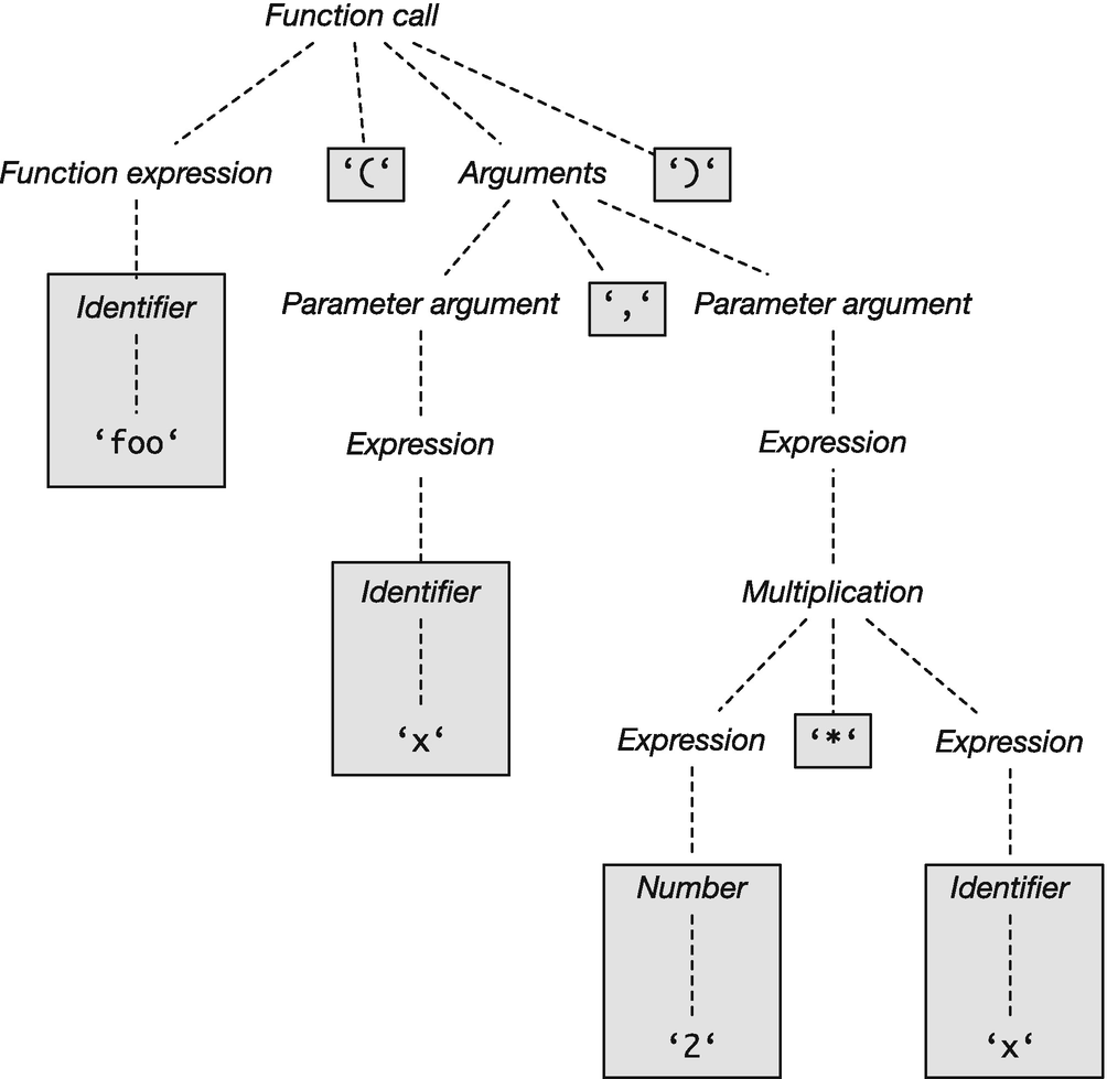
Figure 3-1 Example of an abstract syntax tree for a concrete function call

Grammatical statements are those a parser will consider valid. Such sentences are, if we return to natural languages, those sentences that follow the grammatical rules. This set of grammatical sentences is distinct from the set of sentences that have some associated meaning. It is entirely possible to construct meaningless but grammatically correct sentences. The sentence “Colourless green ideas sleep furiously” is such a sentence, created by the linguist Noam Chomsky. It is entirely grammatical and also completely meaningless. Semantics is the term we use to link grammatical sentences to their meaning. You will know this distinction in programming languages when you run into runtime exceptions. If you get an exception when you run a program, you will have constructed a grammatical sentence—otherwise, the parser would have complained about syntactical errors—but the sentence is violating language rules in some other way. A grammatical sentence does not need to have a well-defined meaning. For example, an expression that adds two variables, x + y, is grammatical, but if the variables contain two incompatible types (x could be a string while y is a number), the sentence violates the language’s type rules. Semantics, when it comes to programming languages, define what actual computations a statement describes. A compiler or an interpreter—the latter for R programs—gives meaning to grammatical statements.³

For embedded DSLs, the semantics of a program is what we do to evaluate an expression once we have parsed it. We are not going to formally specify semantics or implement interpreters, so for this book, the semantics part of a DSL is plain old R programs. More often than not, what we use embedded DSLs for is an interface to some library or framework. It is the functionality of this framework that provides the semantics of what we do with the DSL; the actual language is just an interface to the framework.

Specifying a Grammar

Since we are using R to parse expressions, we do not have much flexibility in what can be considered tokens, and we have some limitations in the kinds of grammars we can implement. However, we have some flexibility for the grammars in how we combine functions and operators.

To specify grammars in this book, I will take a traditional approach and describe them in terms of “rules” for generating sentences valid within a grammar. Consider the following grammar:

EXPRESSION ::= NUMBER
            |  EXPRESSION '+' EXPRESSION
            |  EXPRESSION '*' EXPRESSION
            |  '(' EXPRESSION ')'

This grammar describes rules for generating expressions consisting of the addition and multiplication of numbers, with parentheses to group expressions.

You should read this as “An expression is either a number, the sum of two expressions, the product of two expressions, or an expression in parentheses.” The definition is recursive—an expression is defined in terms of other expressions—but we have a base case, a number, that lets us create a base expression, and from such an expression we can generate more complex expressions.

The syntax I use here for specifying grammars is itself a grammar—a meta-grammar if you will. The way you should interpret it is thus: the grammatical object we are defining is to the left of the ::= object. After that, we have a sequence of one or more ways to construct such an object, separated by |. These rules for constructing the object we define will be a sequence of other grammatical objects. These can be either objects we define by other rules (I will write those in all capitals and refer to them as meta-variables) or concrete lexical tokens (I write those in single quotes, as with the '+' in the second rule for creating a sum). This notation contains the same information as the graphical notation I used in Figure 3-1 where meta-variables are shown in italics and concrete tokens are put in gray boxes.

Meta-grammars like this are used to define languages formally, and there are many tools that will let you automatically create parsers from a grammar specification in a meta-grammar. I will use this home-made meta-grammar much less formally. I use it as a concise way to describe the grammar of DSLs we create or simply a pseudo-code for grammar.

To create an expression, we must follow the meta-grammar rules by using one of the four alternatives provided: either reduce an expression to a number (a sum or product) or create another in parentheses. For example, we can apply the rules in turn and get the following:

EXPRESSION > EXPRESSION '*' EXPRESSION                     (3)
           > '(' EXPRESSION ')' '*' EXPRESSION             (4)
           > '(' EXPRESSION '+' EXPRESSION ')' '*' EXPRESSION (2)
           > '(' number[2] '+' number[2] ')' '*' number[3]  (1x3)

This lets us construct the expression (2 + 2) * 3 from the rules.

If there are different ways to go from meta-variables to the same sequence of terminal rules (there are rules that lead to the exact sequence of lexical tokens), then we have a problem with interpreting the language. The same sequence of tokens could be interpreted as specifying two different grammatical objects. For the expression grammar, we have ambiguities when we have expressions such as 2 + 2 * 3. We can parse this in two different ways, depending on which rules we apply to get from the meta-variable EXPRESSION to the concrete expression. We can apply multiplication first and get what amounts to (2 + 2) * 3, or we can apply the addition rule first and get 2 + (2 * 3). We know from the traditional mathematical notation that we should get the second expression because multiplication has higher precedence⁴ than addition, so the * symbol binds 2 and 3 together tighter than + does 2 and 2, but the grammar does not guarantee this. The grammar is ambiguous.

It is possible to fix this by changing the grammar to this:

EXPRESSION ::= TERM '+' EXPRESSION | TERM
TERM ::= TERM '*' FACTOR | FACTOR
FACTOR ::= '(' EXPR ')' | NUMBER

This is a more complex grammar that lets you create the same expressions, but through three meta-variables that are recursively defined in terms of each other. It is structured such that products will naturally group closer than sums—the only way to construct the expression 2 + 2 * 3 is the parse tree shown in Figure 3-2. The order in which we apply the rules can vary, but the tree will always be this form and group the product closer than the sum.

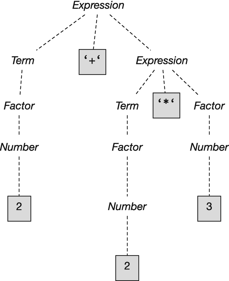
Figure 3-2 Parse tree for 2 + 2 * 3

An unambiguous grammar is preferable over an ambiguous one for obvious reasons, but creating one can complicate the specification of the grammar, as we see for expressions. This can be alleviated by making a smarter parser that takes such things as operator precedence into account or keeps track of context when parsing a string. Regardless of whether we write smarter parsers or unambiguous grammars, we would never work long with expression trees as complex as that shown in Figure 3-2—this tree explicitly shows all grammar meta-variables, but in practice, we would simplify it after parsing it and before processing the expression.

When writing embedded DSLs, we are stuck with R’s parser, and we must obey its rules. If you are writing your own parser entirely, you can pass context along as you parse a sequence of tokens, but if you want to exploit R’s parser and create an embedded DSL, you are better off ensuring that all grammatically valid sequences of tokens unambiguously refer to one grammatical meta-variable. Precedence ambiguities will be taken care of by R as will associativity—the rules mean that 1 + 2 + 3 + 4 is interpreted as (((1 + 2) + 3) + 4). Exploiting R’s parsing rules will allows us to construct languages where each expression uniquely matches a parser meta-variable if we are a little careful with designing the language.

As an example grammar that isn’t just expressions, imagine that we want a language for specifying graphs—graphs as in networks or state machines, not plots. We can define a grammar for directed acyclic graphs (DAGs) by saying that a DAG is either an empty graph or a graph followed by an edge.

DAG ::= 'dag()' | DAG '+' EDGE

We use a function, dag(), to create an empty DAG. Calling this function brings us into the graph specification DSL and gives us an object we can use to program the grammar operations in R. We will use the plus operator to add edges to a DAG. That is a somewhat arbitrary choice, but it makes it easy to implement the parser since we simply will have to overload the generic + function. For edges, we will keep it simple and just require that we have a “from” node and a “to” node. We can define our own infix operator to create them.

EDGE ::= NODE '%=>%' NODE

We cannot define any infix operator we want—we would be out of luck, for example, if we wanted the operator to be ==> since R’s parser would interpret that as two tokens, == and >. We can always define our own, however, if we name them something starting and ending with the percentage sign. We can also reuse the existing infix operators through overloading, as we will do with the plus sign to add edges to a DAG , but for this graph grammar, we can run into some problems if we attempt this, as we will see next. For nodes, we will not expand them more now. They are atomic tokens—we can, for example, require them to be strings.⁵

We will dig more into writing parsers in the next chapter, but for this simple language we can quickly create one. The parser needs to collect edges, so we will use linked lists for this, and it is natural to make an empty DAG contain an empty list of edges. Then, adding edges to a DAG means prepending them to this list. Such an implementation is as simple as this:

cons <- function(car, cdr) list(car = car, cdr = cdr)
dag <- function() structure(list(edges = NULL), class = dag")
`%=>%` <- function(from, to) c(from, to)
`+.dag` <- function(dag, edge) {
    dag$edges <- cons(edge, dag$edges)
    dag
}

With only these four functions, we can create a DAG using syntax like this:

dag() +
  "foo" %=>% "bar" +
  "bar" %=>% "baz"

It might not be the best syntax we can come up with, but it’s easier to read than nested function calls.

add_edge <- function(dag, from, to) {
  dag$edges <- cons(c(from, to), dag$edges)
  dag
}
add_edge(add_edge(dag(), "foo", "bar"), "bar", "baz")

Using the pipe operator from magrittr might be even more readable, though, for people familiar with it.

dag() %>% add_edge("foo", "bar") %>% add_edge("bar", "baz")

In any case, we have built a small language that we can parse by defining only four functions—three if we discount the list cons function, which isn’t specific to the language.

We used %=>% to construct edges. Could we use => instead? The short answer is no. R’s parser will consider this two tokens, = and >, and although we could define a function with that name, using backquotes to make it a valid identifier, we wouldn’t get an infix operator.

`=>` <- function(from, to) c(from, to)
`=>`("foo", "bar")
"foo" => "bar"

## Error: <text>:3:8: unexpected '>'
## 2: `=>`("foo", "bar")
## 3: "foo" =>
##           ^

If we want to have an infix operator that does not use percentage signs, we have to overload one of the operators that R already has—and => is not one of them (greater-than-or-equal is >=).

Could we use > instead then? This is an R infix operator, and, therefore, we can overload it. We just need a type for a node to do this. If we keep nodes specified as strings, we would have to change the string operator, and we do not want to do that—it could potentially break a lot of existing code—so the best approach would be to define a node class to work with.

node <- function(name) structure(name, class = "node")
`>.node` <- function(from, to) c(from, to)

With these functions, we can create an edge with this syntax:

node("foo") > node("bar")

## [1] "foo" "bar"

Changing a % infix operator to > changes the precedence, however. A % operator has higher precedence than +, which is why we got edges that we could add to the DAG earlier, but > has lower precedence than +, so we add the left node to the DAG first and only then invoke the > operator.

dag() + node("foo") > node("bar")

## $edges
## $edges$car
## [1] "foo"
## attr(,"class")
## [1] "node"
##
## $edges$cdr
## NULL
##
##
## [[2]]
## [1] "bar"

We can fix this using parentheses, of course.

dag() + (node("foo") > node("bar"))

## $edges
## $edges$car
## [1] "foo" "bar"
##
## $edges$cdr
## NULL
##
##
## attr(,"class")
## [1] "dag"

It is not particularly safe to rely on programmers to remember parentheses, so a better solution is to get the precedence right. We can do that by choosing a different operator for adding edges to DAGs . If we replace + with |, for example, we get the right behavior since | has lower precedence than >.

`|.dag` <- function(dag, edge) {
  dag$edges <- cons(edge, dag$edges)
  dag
}
dag() | node("foo") > node("bar")

## $edges
## $edges$car
## [1] "foo" "bar"
##
## $edges$cdr
## NULL
##
##
## attr(,"class")
## [1] "dag"

There are pros and cons to using operator overloading. Having to change string tokens into node tokens requires more typing, but on the other hand, we can use this to validate expressions while we parse them and make sure that nodes are strings.

Alternatively, we could use meta-programming and explicitly traverse expressions to make sure that the > operator will be the edge-creating operator instead of string comparison, similar to how we rewrote matrix expressions in the previous chapter.

Returning to the magrittr solution for a brief moment, I think it is worth mentioning that designing a language is not all about defining new syntax. The language we are defining here, for specifying graphs, is doing the same as the pipe operator does, so in this particular case, we do not need to specify a new grammar to get all the benefits we want to achieve. When using pipes, we avoid the nested function calls that would make our code hard to read, and we can specify a DAG as a list of edges that we add to it. The pipe operator will be familiar to most programmers, and best of all, if we use it, we do not need to implement any parsing code. We are still creating a DSL, though, when we define the functions to manipulate a DAG . Providing functions that give you a vocabulary to express domain ideas is also language design. The dplyr package is an example of this—it is used together with the pipe operator to string various operations together, so it does not provide much in terms of new syntax, but it provides a very strong language for specifying data manipulation.

Of the various solutions we have explored, I prefer the pipe-based. It makes it easy to extend edge information to more than a “from” node and a “to” node—which is hard with a binary operator—and we can implement it without any language code; we just have to make the DAG the first argument to all the manipulation functions we would add to the language. Of course, this solution is possible only because the language we considered was a simple string of operations. This is not always the case, so sometimes we do need to do a bit more work.

Designing Semantics

The reason we write domain-specific languages is to achieve some effect—we want to associate meaning, or semantics, to expressions in the DSL, and we want our DSL expressions to achieve some result, whether that is by executing some computations or by building some data structures. The purpose of a DSL merely is to provide a convenient interface to whatever semantics we want the language to have.

If we always make our parsing code construct a parse tree, then the next step in processing the DSL involves manipulating this tree to achieve the desired effect. There might be several steps involved in this—for example, we rewrote expressions in the matrix expression example to optimize computations—but at the end of the processing we will execute the commands the DSL expression describes.

Executing the DSL is sometimes straightforward and can be done as a final traversal of the parse tree. This is what we did with the matrix expressions where the purpose of the DSL was to rewrite expressions rather than evaluate them—the latter being a simple matter of multiplying and adding matrices. In other cases, it makes sense to separate the semantic model and the DSL by having a framework for the actions we want the language to execute. Having a framework for the semantics of the language lets us develop and test the semantic model separately from the language we use as an interface for it; it even allows us to have different input languages for manipulating the same semantic model—not that I recommend having many different languages to achieve the same goals.

To illustrate this, we can consider a language for specifying a finite state continuous time Markov chain (CTMC).⁶ I chose this example because we have already implemented several versions of a finite state system when we implemented the graph DSL, and for a CTMC we just have to associate rates with all the edges. Continuous time Markov chains are used many places in mathematical modeling, and the implementation mostly comes down to specifying an instantaneous rate matrix. This is a matrix that specifies the rate at which we move from one state to another. Such a matrix should have non-negative values on all off-diagonal entries, and on the diagonal, we should have minus the sum of the other entries in the rows. In a framework where we use CTMCs, we would likely implement the functionality to work on rate matrices, but for specifying the CTMCs, a domain-specific language might be easier to use.

Calling it the “semantics” of the language to translate graph specifications into a matrix might be stretching the word, but if we consider the DSL as a way of specifying models and the (imagined) framework that manipulates them as part of the language, then I think we can justify it. Using the language will consist of specifying the CTMC, translating it into the corresponding rate matrix, and then manipulating it as intended. The language part of it is the translation from the specification into a matrix.

As for the graphs shown previously, we need to specify the edges in the chain. We need to have a rate associated with each edge, so the most natural syntax will be the pipe version—with this version it is simpler to specify three values for an edge: the “from” and “to” states and the rate. I will keep these in three different linked lists, just because it makes it easier to construct the matrix this way.

We reuse these two functions we wrote in the previous chapter:

cons <- function(car, cdr) list(car = car, cdr = cdr)
lst_length <- function(lst) {
  len <- 0
  while (!is.null(lst)) {
    lst <- lst$cdr
    len <- len + 1
  }
  len
}
lst_to_list <- function(lst) {
  v <- vector(mode = "list", length = lst_length(lst))
  index <- 1
  while (!is.null(lst)) {
    v[[index]] <- lst$car
    lst <- lst$cdr
    index <- index + 1
  }
  v
}

We then define the following functions for specifying CTMCs:

ctmc <- function()
  structure(list(from = NULL,
                 rate = NULL,
                 to = NULL),
            class = "ctmc")

add_edge <- function(ctmc, from, rate, to) {
  ctmc$from <- cons(from, ctmc$from)
  ctmc$rate <- cons(rate, ctmc$rate)
  ctmc$to <- cons(to, ctmc$to)
  ctmc
}

Translating the lists into a rate matrix is now simply a normal programming job. We collect the nodes from the “from” and “to” lists—we translate them into R lists first since those are easier to work with once we are done collecting elements—and we then get the unique node names. These become the rows and columns of the rate matrix, and we iterate through all the edges to insert the rates. After that, we set the diagonal, and we are done.

rate_matrix <- function(ctmc) {
  from <- lst_to_list(ctmc$from)
  to <- lst_to_list(ctmc$to)
  rate <- lst_to_list(ctmc$rate)
  nodes <- c(from, to) %>% unique %>% unlist

  n <- length(nodes)
  Q <- matrix(0, nrow = n, ncol = n)
  rownames(Q) <- colnames(Q) <- nodes

  for (i in seq_along(from)) {
    Q[from[[i]], to[[i]]] <- rate[[i]]
  }

  diag(Q) <- - rowSums(Q)

  Q
}

Constructing a CTMC rate matrix using this small language is now as simple as this:

Q <- ctmc() %>%
  add_edge("foo", 1, "bar") %>%
  add_edge("foo", 2, "baz") %>%
  add_edge("bar", 2, "baz") %>%
  rate_matrix()
Q

##     bar foo baz
## bar  -2   0   2
## foo   1  -3   2
## baz   0   0   0

Once we have translated the CTMC into this matrix, we can consider the language design over. However, integrating CTMC construction and the operations that we can do on a CTMC will be important for ease of use of the DSL and can be considered part of the language as well. In this particular case, the good news is that the actual language design is done for us. The pipe operator tells us how to combine our CTMCs with further processing—we just have to write functions that can be used in a pipe. For example, if we want to know the transition probabilities of the CTMC over a time interval—i.e., we want to know the probability of going from any one state to any other over a given time—we can add a function for that. The probabilities can be computed using matrix exponentiation (if you are not familiar with CTMC theory, just trust me on this). To make such a function compatible with a pipeline, we simply have to make the most likely data to come from the left in a pipe the first argument of the function. So, we could write this:

transitions_over_time <- function(Q, t) expm(Q * t)
P <- Q %>% transitions_over_time(0.2)
P

## 3 x 3 Matrix of class "dgeMatrix"
##           bar       foo     baz
## bar 0.6703200 0.0000000 0.32968
## foo 0.1215084 0.5488116 0.32968
## baz 0.0000000 0.0000000 1.00000

Even with the language constructions in place—the pipe operator—there is still some language design to be done. It is not always obvious what the flow of data will be through a pipe after all. An example is when we want to evolve vectors of state probability.

probs <- c(foo=0.1, bar=0.9, baz=0.0)

Is it more natural to have the probability vectors flow through the pipeline?

evolve <- function(probs, Q, t) {
  probs <- probs[rownames(Q)]
  probs %*%transitions_over_time(Q, t)
}
probs %>% evolve(Q, 0.2)

## 1 x 3 Matrix of class "dgeMatrix"
##            bar        foo     baz
## [1,] 0.6154389 0.05488116 0.32968

Or, would it be more natural to always have the CTMC (or its rate matrix) flow through the pipeline?

evolve <- function(Q, t, probs) {
  probs <- probs[rownames(Q)]
  probs %*%transitions_over_time(Q, t)
}
Q %>% evolve(0.2, probs)

## 1 x 3 Matrix of class "dgeMatrix"
##            bar        foo     baz
## [1,] 0.6154389 0.05488116 0.32968

The former might feel more natural if we think of the system evolving over time, but the latter would fit better with a pipeline where we construct the CTMC first, then translate it into a rate matrix, and finally evolve the system.

ctmc() %>%
  add_edge("foo", 1, "bar") %>%
  add_edge("foo", 2, "baz") %>%
  add_edge("bar", 2, "baz") %>%
  rate_matrix() %>%
  evolve(0.2, probs)

## 1 x 3 Matrix of class "dgeMatrix"
##            bar        foo     baz
## [1,] 0.6154389 0.05488116 0.32968

Only use cases and experimentation will tell us what the best language design is. But then, that is also what makes designing languages so interesting.