Chapter 10
Computational Fluid Dynamics Modeling
Tutorial and Examples
G. Landucci1, M. Pontiggia2, N. Paltrinieri3,4, and V. Cozzani5 1University of Pisa, Pisa, Italy 2D'Appolonia S.p.A., San Donato Milanese (MI), Italy 3Norwegian University of Science and Technology (NTNU), Trondheim, Norway 4SINTEF Technology and Society, Trondheim, Norway 5University of Bologna, Bologna, Italy
Abstract
This tutorial is aimed at demonstrating the capabilities of computational fluid dynamics (CFD) models in capturing complex dynamic scenarios. In particular, the focus is on the dispersion of flammable heavy gas in urban areas. The necessary steps for carrying out a dispersion study on a large scale are described. The methodology is applied for the analysis of a case study: the accident in Viareggio, Italy, in 2009, in which a flash fire occurred after the derailment of a freight train. It shows how CFD models allow effective reproduction of large-scale release and dispersion events in the presence of a congested and complex environment. In parallel, limitations of conventional approaches are also shown for the same case study.
Keywords
CFD models; Dynamic consequence analysis; Heavy gas dispersion modeling; LPG; Viareggio accident
1. Introduction
In this chapter, the potential of computational fluid dynamics (CFD) simulations in supporting dynamic risk assessment is presented. The aim is to demonstrate the advanced features of CFD tools, allowing for more comprehensive analysis of accident scenarios with respect to conventional models based on integral approaches.
This chapter is devoted to the assessment of release and dispersion of liquefied petroleum gas (LPG) in an urban context through the analysis of a specific case history: The accident in Viareggio, Italy, in 2009 is used as a reference case study [1]. The accident followed a freight train derailment in which an LPG tank car was punctured, releasing its entire content. The ignition led to a severe flash fire, with consequent extended property damages and 32 fatalities.
The methodology adopted for setting up the CFD model is shown to highlight the complexity of the tool as well as the level of detail needed to carry out a real-scale consequence assessment study. The application of conventional integral models, in particular the unified dispersion model (UDM) [2], is presented as well. The results of the calculation are compared with the reported damages, presenting indications for the selection of the proper modeling strategy in the perspective of dynamic risk assessment.
2. Methodology Tutorial
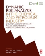
Fig. 10.1 shows the flowchart of the approach and generic requirements needed to perform the CFD study. The figure also shows the alternative path needed for setting up the same type of simulation by adopting integral tools, which reduces the simulation to only two steps (ie, steps 1 and 5 in Fig. 10.1).
The preliminary step (step 0) of a CFD study consists of the determination of the scenario to be analyzed. This is a crucial step because setting up CFD requires relevant resources, in terms of both man-hours and computational resources. Chapter 9 discusses the selection criteria for a proper modeling strategy to limit the number of cases to be assessed with CFD tools. Hence, the preliminary phase is out of the scope of this chapter.
This tutorial focuses on the application of CFD models for the analysis of a scenario: flammable gas dispersion in complex environment, such as urban areas, by performing a three-dimensional study. The aim of dispersion studies for flammable materials is the evaluation of the extension and features of the flammable cloud, that is, the zone in which the concentration of the released gas is between the flammable limits (lower flammability limit [LFL] and upper flammability limit [UFL]) [3].
The first step (step 1) is to retrieve input information to (1) characterize the surrounding environment and (2) determine the source term of the released substance. The surrounding environment needs to be characterized by determining the meteorological conditions during the dispersion scenario and the features of the territory in which the dispersion takes place. Wind and atmospheric stability play an important role in the dispersion study (see Lees [3] for more details) and may significantly change, affecting the direction and shape of the flammable cloud. For evaluation of the released substance source term, information about the release size (eg, the equivalent release diameter) and operative data prior to the loss of containment (eg, pressure, temperature, composition, and inventory of the hazardous substance) from a tank or other detention system are needed [3,4]. Based on this information, CFD tools may simulate the outflow of the substance, or the source term can be directly set up by the user as an “input mass” condition [5]. In the latter case, integral models for source terms [4] may also be used to limit the computational resources for the CFD simulation, as explained in Section 3.2.1.
As shown in Fig. 10.1, the information in step 1 constitutes the basis for performing simulation through integral modeling, thus obtaining the results in terms of iso-concentration contours. Instead, CFD models need several additional steps, which are described in detail for the case under analysis.
Step 2 is aimed at defining the domain in which the simulation needs to be carried out, obtaining a three-dimensional spatial representation of the geometrical environment. ANSYS ICEM (ANSYS, Inc., Canonsburg, PA) [5] or other generic computer-assisted design tools may be adopted for defining and drawing the geometry. Step 2 supports the definition of the computational grid (step 3), which is needed in commonly applied software for CFD modeling (such as ANSYS Fluent (ANSYS, Inc., Canonsburg, PA) [5]) adopting the finite volume approach. The computational grid (or mesh) is obtained from the subdivision of the three-dimensional space into control volumes, in which the governing equations (conservation of mass, energy and momentum and radiative heat transfer equation) are solved. In this step, solution and discretization methods are also selected, depending on the type of problem, to achieve the optimal and stable solution convergence. More details on this topic are extensively reported elsewhere [5–8].
Once the numerical set-up of the problem is carried out, boundary conditions need to be specified. Boundaries direct motion of flow, specifying solid (eg, ground, obstacles, buildings, and vegetation) and fluid zones (in the case of a dispersion study, the portion of the domain occupied by atmospheric air and the gas-flammable or toxic substance). Typical boundary conditions for dispersion studies are summarized in Table 10.1.
Finally, the simulation can be run to obtain the final results (step 5). As mentioned earlier, the key outcome of a dispersion study of flammable gases is the obtainment of a dynamic concentration profile. With respect to integral models, CFD allows advanced types of profiles, such as streamlines or velocity vectors distribution. This allows the obtaining of information on the influence of obstacles on fluid motion.
3. Application of the Approach
3.1. Description of the Case Study
In this section, the potentialities for CFD in analyzing the dynamic evolution of a large-scale flammable cloud in a congested urban area are shown through the analysis of a case study. In particular, the consequence analysis of the release event following the Viareggio train accident is presented.
On June 29, 2009, a freight train was carrying 14 LPG tank cars through the densely populated area of Viareggio at a speed of 90 km/h. A tank car derailed, overturned, and was punctured, releasing its entire content. LPG vaporized and formed a cloud that spread over the railway area and extended over a residential zone near the railway. A flash fire followed the cloud ignition, causing extended damages [9]. In some locations, LPG vapors penetrated into enclosed zones, such as houses and an underground garage, leading to a confined explosion following ignition.
Table 10.1
Examples of Boundary Conditions Adopted in Gas Dispersion Studies Carried Out by Computational Fluid Dynamics Models
| Type of Element | Schematization | Type of Boundary Condition |
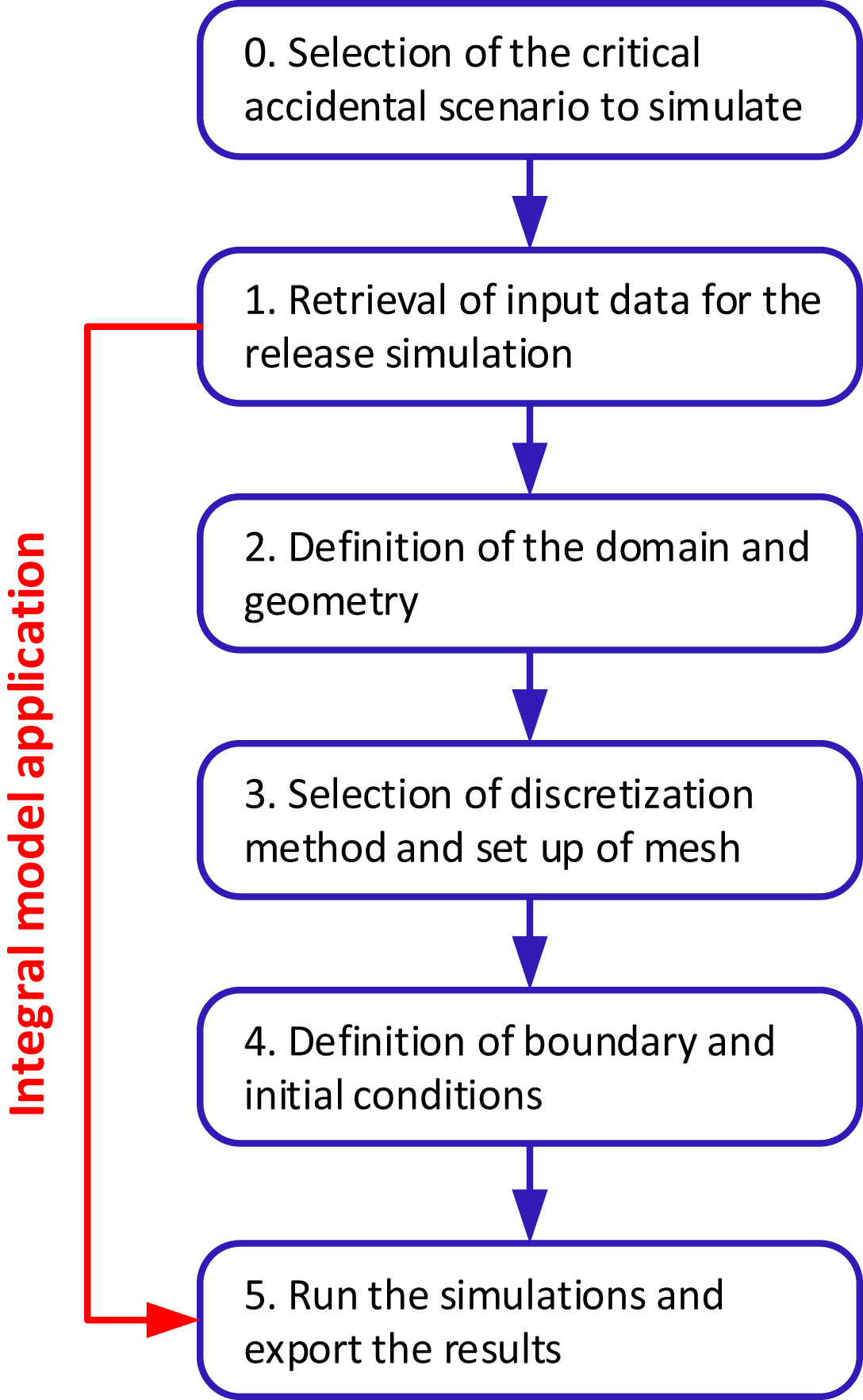
| Inlet of the substance in the domain | 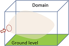 | Because the gas is characterized by compressible flow, mass or pressure inlet can be typically adopted [5]. Source term may be calculated with integral models [4] and imposed by the user to limit computational efforts. Temperature and turbulence of the inlet mass are assigned as well. |
| Outlet from the domain |  | Pressure outlet is typically adopted, defining the static/gauge pressure at the outlet boundary. This is interpreted as the static pressure of the environment into which the flow exhausts. |
| Surrounding air and wind inlet |  | As a result of low speed (subsonic conditions), incompressible flow may be assumed, imposing a velocity profile, temperature, and turbulence values for the inlet wind flux. |
| Ground and obstacles |  | No-slip boundary condition is commonly applied considering a solid “wall” for the ground, obstacles, buildings, etc. This is used to bound fluid and solid regions. Roughness and temperature are also specified. |

A detailed analysis of the consequences of the fire has also been carried out, taking into account a systematic classification of damages. The following types of target have been considered: structures/houses, vehicles, and vegetation. Three types of damage, with increasing severity, have been identified [1]: (1) radiation damage due to distant radiation; (2) moderate flame damage due to flame engulfment with significant effects on grass/hedges and poor effects on buildings; and (3) severe flame damage (grass/vegetation set on fire, buildings or cars set on fire, rupture of windows due to strong thermal dilatation). For the sake of brevity, an example of the increasing level of damages is shown for vehicles and buildings in Fig. 10.2.
This series of events having extremely severe consequences is a typical example of the hazard posed by accident scenarios in LPG transportation by road and rail [10,11]. Dynamically modeling the consequences of such accidental scenarios is the only way to foresee the impact area to design appropriate mitigation measures and to prepare specific emergency plans based on the expected impact area of such accidents [12,13].
To reproduce the effects of the accident, a CFD model was applied. The model performance was analyzed in detail by a critical comparison of CFD simulation results with the damage map obtained by analyzing the effects of fire on buildings, vehicles, and vegetation [1]. More details about model development and set-up are reported elsewhere [1,9,14]. Here the relevant aspects are summarized to highlight the possible advanced features associated with the implementation of a CFD model to analyze the dynamic evolution of accident scenarios. Moreover, the set-up of conventional integral models [2] is shown, and the results of the two modeling approaches are compared.
3.2. Simulation Settings
3.2.1. Computational Fluid Dynamics Model
The geometry of the area of interest was imported into the CFD code from a topographical database available for Viareggio [15]. The database allowed fast and easy geometry generation: The perimeter at the eaves' height and the position were available for each building, and buildings were simulated extruding top area to the ground, leading to simplified representation of the urban terrain as a combination of parallelepiped structures. Edges smaller than 0.2 m, that is, the smaller dimension documented in the topographical database, were smoothed to remove relatively small details that would require high grid refinement but would play a minor role in gas dispersion. Further details on the geometry import procedure can be found elsewhere [16].
The domain area is represented in Fig. 10.3A, featuring a total extension of 350 × 500 × 45 m. Fig. 10.3 displays the schematization used to represent the actual geometry in the CFD code. Fig. 10.3B shows some details added to the imported geometry, such as containment walls present along the railway as well as the footbridge. Wall thickness was assumed constant and equal to 0.2 m, and the slope of the stair flights was set equal to 45 degree to reduce mesh skewness. Trees were added in the most densely packed zone (see an example in Fig. 10.3B), whereas isolated trees were not considered owing to their low influence on the dispersion of the gas. Average tree dimensions were obtained through direct onsite measurement and were used in the geometry generation. Each single tree was modeled as a solid body, therefore being not permeable to the gas.
Tank cars (apart from the punctured one) and train engine were modeled as boxes 16 m long, 3 m wide, and 3 m high. The overview of the tank car's position is reported in Fig. 10.3A. The punctured tank car was reproduced with a higher level of detail. A cylindrical tank and wheel axle encumbrance were represented. Roadbed was also reproduced, imposing a standard slope and width. Details of tank car geometries are reported in Fig. 10.3B.
Buildings were considered solid; therefore, no gas penetration was simulated. The garage in which a partially confined explosion occurred was represented as a cavity in the ground. Access pads were also reproduced to investigate the behavior of the dense cloud in correspondence with the slope and to check the capability of the CFD code to forecast a gas infiltration large enough to justify the gas explosion (see Fig. 10.3C).
From the punctured tank, a flashing liquid was assumed to enter the atmosphere, leading to the formation of a gas jet (from the flash fraction) and of an evaporating pool (from the liquid rainout). Gas inlet surface (into the integration domain) was obtained on the lateral surface of the cylindrical tank, at its axial end, facing downward and impinging on the ground, in agreement with reported tank damage and with the tank position after the accident. PHAST software (DET NORSKE VERITAS (DNV), London, UK) [17] was adopted for both jet and pool simulation, assuming saturated liquid at atmospheric temperature inside the tank car. The CFD simulation boundary conditions were in this case preelaborated through integral modeling to optimize the computational resources.
A triangular unstructured grid was imposed over the buildings, with a characteristic length of half the smaller edge up to a maximum of 1 m. A 0.05-m triangular grid was imposed on the gas inlet surface, whereas a 0.2-m grid was used at ground level near the source to describe pool evaporation. A size function was set with a growth factor of 1.2 and a size limit of 20 m, leading to a tetrahedral unstructured grid of about 8 million elements (see Fig. 10.3D and E for some mesh details). Each simulation required about 40 h on a 16-parallel-processes cluster.
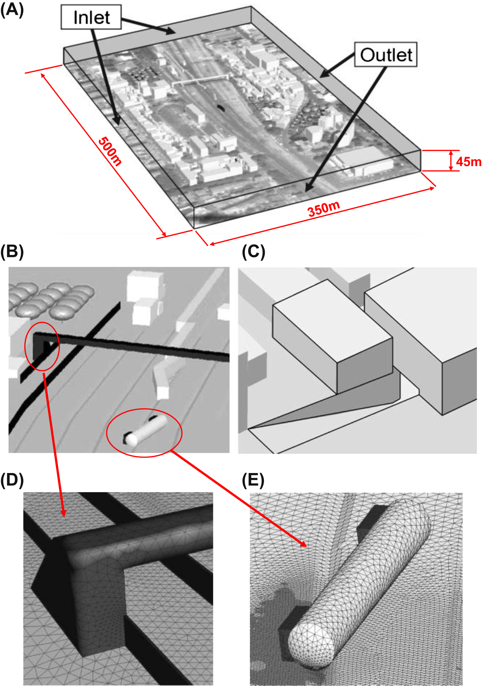
Figure 10.3 Geometry and mesh adopted for the simulation of Viareggio liquefied petroleum gas dispersion. (A) Overview of the domain and boundary definition; (B) schematization of footbridge, walls, trees, and train added to the imported geometry; (C) details of buildings and of an underground garage; (D) mesh definition details for the footbridge; and (E) mesh definition details for the derailed tank car.
3.2.2. Integral Models
In the analysis of potential consequences of hazardous material releases carried out for quantitative risk assessment, simplified models are used owing to the wide areas to analyze and the uncertainty affecting the release position and features [18]. Thus, in general, source-point concentrated parameter dispersion models are used to model gas dispersions.
Dispersion simulations were carried out using UDM as implemented in the PHAST software. More details on implementation and UDM description are reported elsewhere [17]. Two main alternative simulation hypotheses were considered in the present study: (1) simulation of a continuous horizontal LPG release considering an average surface roughness typical of building area (= 1 m), and (2) puff release of 25,000 kg of LPG (initial condition at tD is stoichiometric mixture with air), with low wind speed (2 m/s in stability class F, blowing from west to northwest).
3.3. Results and Discussion
Fig. 10.4 shows the results of the CFD simulation at 300 s. In Fig. 10.4A, model predictions have been superimposed over the maps of the observed damages (iso-concentration footprint), classified according to the rules defined in Section 3.1. The figure shows that almost all the “severe” and “moderate” damage points are within (or very close to) the predicted LFL boundary, therefore validating the predictive capabilities of the CFD model used.

Figure 10.4 Computational fluid dynamic results obtained for liquefied petroleum gas dispersion in urban area. (A) Predicted extension of flammability limits 300 s after the release compared to observed damages; (B) details of the dispersion study on the east side of the station; (C) details of the dispersion study on the west side of the station showing the flammable cloud descending into the garage where a confined explosion occurred. C, concentration of liquefied petroleum gas; LFL, lower flammability limit; UFL, upper flammability limit.
Few severe and moderate damage points lay outside the LFL boundary. Nevertheless, those are included in the zone where concentrations are above the value of LFL/2. This boundary, which is only a few meters wider than the LFL boundary, is proposed by several technical standards to conservatively identify the maximum extension of the region affected by flash fire damage. As an example, Fig. 10.4B shows the concentration profiles at ground level in a garden on the east side of the railway (see Fig. 10.4A for the location in the area), where moderate flame exposure was identified. As shown in the figure, although the predicted concentrations are lower than the LFL boundary, almost all the garden is adopted by predicted concentration values between LFL and LFL/2, which fully envelope all the severe and moderate damage points.
Similarly, Fig. 10.4C shows the concentration profiles close to the underground garage in which a partially confined explosion was reported (see Fig. 10.4A for the location in the area). In the figure, the walls of the buildings over the garage were rendered partially transparent to allow the visualization of the concentration field inside the garage. The predicted concentration values in the garage are larger than LFL/2 limits, and the LFL boundary is only a few meters from the observed damages. If compared with the cloud dimensions, which are on the order of a few hundred meters, there is good agreement between the reported damages and the CFD model simulation.
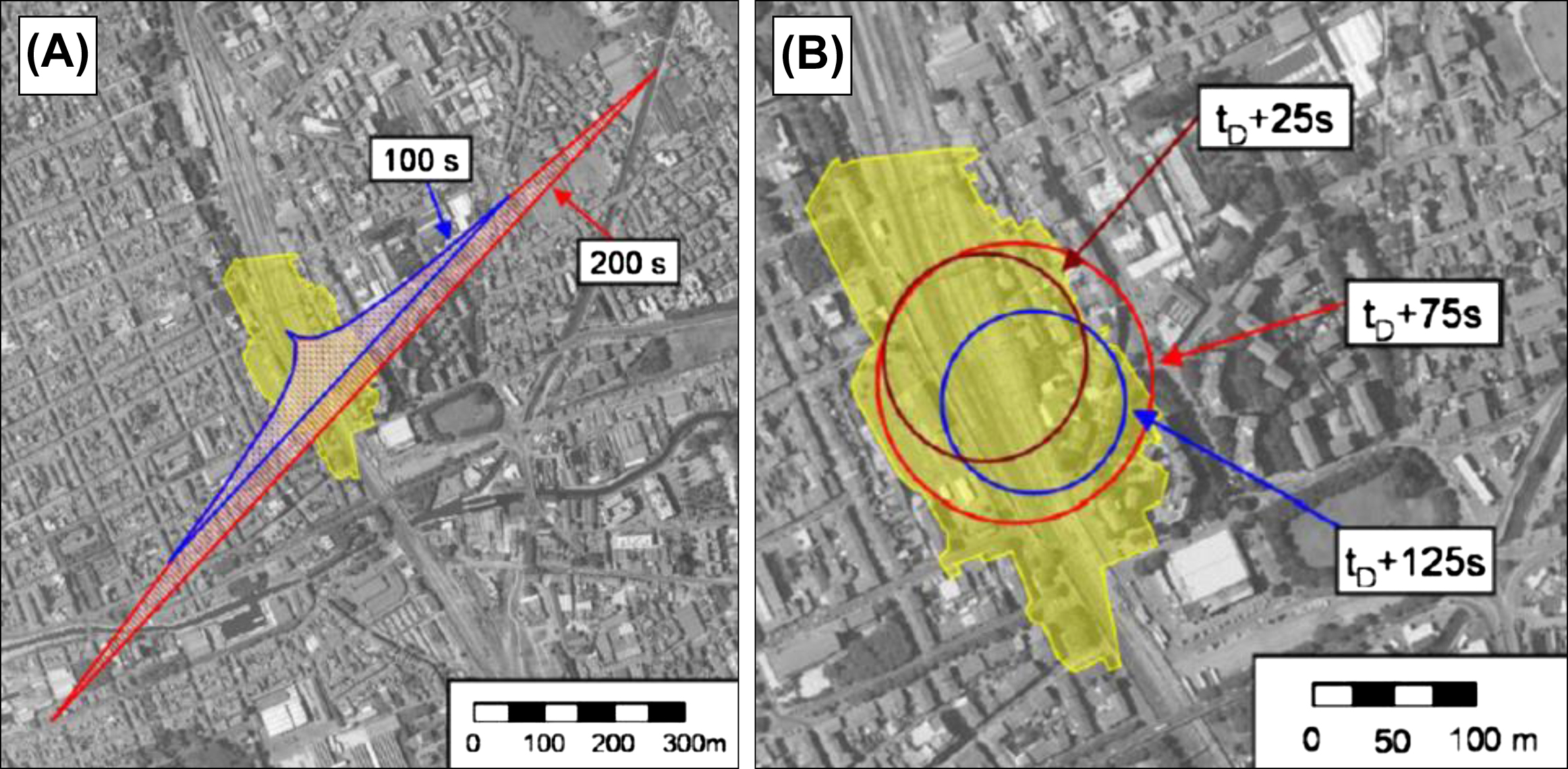
Figure 10.5 Examples of results in the simulation for the Viareggio dispersion by alternative simulation hypothesis. (A) Lower flammability limit per two contours for continuous horizontal release, surface roughness typical of building area (z0 = 1 m); (B) lower flammability limit contours at three simulation times for puff release of 25,000 kg of liquefied petroleum gas (initial condition at tD is stoichiometric mixture with air). Yellow marks (white in print versions) the area actually intersected by damage in the accident. Wind direction was west to northwest. Adapted from Landucci G, Tugnoli A, Busini V, Derudi M, Rota R, Cozzani V. The viareggio LPG accident: lessons learnt. Journal of Loss Prevention in the Process Industry 2011;24:466–476. doi:10.1016/j.jlp.2011.04.001.
In the case of a simulation carried out with integral models, the results are rather different from the actual records. Fig. 10.5 reports some results obtained for different simulations carried out using UDM as implemented in the PHAST software [17]. As shown in the figure, different assumptions about release conditions and atmospheric dispersion (introduced to allow the application of these simplified models) lead to quite different results. All the alternative approaches lead to conservative results. The results can also be very conservative, leading to very large impact areas with a consequent waste of resources when emergency plans have to be prepared.
Moreover, it is worth mentioning that CFD allows identifying and analyzing a scenario that cannot be captured by conventional static approaches. In particular, as shown in Fig. 10.4C, because flammable concentrations are predicted in the underground garage, the possibility of confined explosion introduces a novel scenario besides the flash fire, thus demonstrating the capabilities of CFD in supporting dynamic hazard and risk assessment.
4. Conclusions
In this tutorial, the potential of CFD models in simulating large-scale dispersion scenarios is analyzed in the perspective of dynamic risk assessment. In particular, the consequences of the Viareggio accident involving a flash fire due to LPG release and vaporization following a train derailment have been simulated in detail.
The good agreement found between the actual observed damages and the predictions obtained using the CFD approach strongly supports the reliability of the CFD approach for simulating heavy gas dispersion in geometrically complex environments. Moreover, the results shown with the static integral model approach appear extremely conservative, leading to an overestimation of consequences in the far field.
The advanced features of CFD models may foresee the evolution of accidental scenarios that may evolve into additional accidents, such as the confined explosion in the garage captured by the dispersion study, demonstrating the importance of CFD studies in the framework of dynamic consequence and risk assessment.
..................Content has been hidden....................
You can't read the all page of ebook, please click here login for view all page.