
In this work, relative service differentiation that targets a particular ratio of network QoS parameters among service classes is implemented using packet-forwarding mechanisms. However, due to the dynamics of queue lengths (e.g., rapid fluctuation of data traffic), the packet-forwarding mechanisms may not be able to maintain the targeted network QoS ratios during all time windows.
Under the relative DiffServ paradigm, this chapter carries the QoS mapping framework of Chapter 3 further and applies QoS mapping in the queueing system, where the relative differentiated service is implemented through packet-forwarding mechanisms. But, unlike our discussions in Chapter 3, in this chapter, we will observe the end-to-end, application layer performance of QoS mapping under conditions of less ideal network layer performance with regard to QoS proportionality.
Different packet-forwarding mechanisms result in different qualities in terms of network performance QoS ratios, and different network performance QoS ratios in turn affect the end-to-end, application layer performance that results from QoS mapping. In this context, our discussion will include packet-forwarding mechanisms such as queueing disciplines and packet dropping rules. In particular, we will seek a mechanism that results in “persistent” relative differentiation among classes, that is, the ability to preserve the target ratio of network layer performance averaged over a wide range of time scales.
The remainder of this chapter is organized as follows. The adaptive packet-forwarding mechanism is proposed in Section 4.2, it is designed to support a stable and persistent network QoS (i.e., DS) level on the basis of a combination of the commonly accepted active queue management (AQM) scheme known as RED [45] and a scheduling scheme known as WFQ [22]. Section 4.3 describes QoS mapping scenarios based on single- or multiple-queue network nodes.[1] Performance assessment using NS [27] and error-resilient ITU-T H.263+ bit streams is given in Section 4.4, where experimental results are also discussed. Concluding remarks are given in Section 4.5.
In this section, we present a packet-forwarding mechanism that provides fairly persistent network service differentiation in the QoS tuple {delay, loss}, even if the network load condition is time-varying. A well-known candidate for the required packet-forwarding mechanism is one based on the popular WFQ, which is already being deployed in some Cisco routers for IP QoS. However, previous work [113], [114] shows that WFQ with static weighting factors (static WFQ) is not capable of providing persistent service differentiation in finer time scales. Proprietary scheduling has instead been proposed for proportional DiffServ [32], [33], thus limiting the practical usability comparison with WFQ that manufacturers accepted and widely used. Thus, in this chapter, we propose to use adaptive WFQ rather than static WFQ in combination with RED (or RIO) [42], [97].
WFQ provides a weighted portion of the shared bandwidth to each class queue in accordance with its weighting factor. Within each class queue, RIO can adjust drop rates through a drop probability control algorithm using a RIO parameter set consisting of the minimum threshold, maximum threshold, and maximum drop probability (minth, maxth, maxp) for each IN or OUT control curve, respectively. In a similar manner, to provide differentiated services on distinct classes persistently, we suggest observing the already admitted traffic and adapting to the dynamic network conditions. From among several network status indices, such as packet loss rate, RTT, and filtered queue length, we selected filtered queue length and its change rate. Then, focusing on the proportional packet loss/delay differentiation, we devised the control loop algorithm illustrated in Figure 4.1.
Figure 4.1. Control loop for the proposed proportional loss/delay service di. erentiation (adaptive WFQ).
In our algorithm, to maintain proportional loss/delay differentiation, WFQ weighting factors with RIO are dynamically adjusted. Service delays and loss ratios between DS levels (classes) should depend on the allocated portions of shared bandwidth at each time interval. In proportional Diffserv, the desired differentiation among M class queues can be quantified as the ratios δi, i = 0, 1, . . . , and M – 1, as in Eq. (4.1). We found that the measured loss rate and delay both depend heavily on the weighting factor wi(t) of WFQ. The drop rate for each DS level can be proportionally adjusted by setting the RIO parameters (minth, maxth, maxp) without frequent updating because average queue length reflects the queue build-up condition. Then, it is sufficient to change wi(t) dynamically to achieve our goal of obtaining stable and persistent service differentiation.
The proportional differentiation of delay (di) and loss (li) can be stated as

To provide the desired differentiation, the adaptive weighting factors of WFQ, wi(t), i = 0, 1, . . . , and M – 1, used in time interval [t, t + Δ τ], are

where ![]() is the filtered queue length at time t. With the assumption
is the filtered queue length at time t. With the assumption ![]() , we have
, we have

Then, we can obtain the adaptive weighting factors via

Table 4.1. Performance Comparison Between Static WFQ and Adaptive WFQ
Classes | Static WFQ | Adaptive WFQ | ||||||
|---|---|---|---|---|---|---|---|---|
AF1 | AF2 | BE | AF1 | AF2 | BE | |||
Delay (msec) | 11.8 | 17.6 | 33.1 | 10.7 | 18.5 | 35.2 | ||
Deviation (msec) | 11.78 | 17.37 | 22.33 | 9.96 | 15.53 | 57.27 | ||
Delay Ratio Between Classes | 1.49 | 1.88 | 1.73 | 1.91 | ||||
Loss Rate (%) | 6.2 | 11.4 | 34.0 | 6.1 | 11.5 | 25.6 | ||
Loss Ratio Between Classes | 1.84 | 2.98 | 1.89 | 2.23 | ||||
To demonstrate the effectiveness of the proposed adaptive forwarding, the loss/delay differentiation performance of static and adaptive WFQ is compared by NS. Comparison is conducted for a shared node with three class queues (AF1, AF2, and BE) with a 4:2:1 proportional differentiation target. To generate network loads, each queue was injected with five TCP and five UDP (jittered CBR) flows with identical characteristics. The results were tabulated in Table 4.1, with the delay, delay deviation, and loss rate being averaged over the entire trace of the simulation. The results show that the proposed forwarding scheme with adaptive WFQ has delay and loss rate ratios closer to the target ratio of 4:2:1.
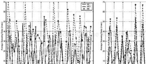
The average queuing delays calculated per 100 received packets are depicted in Figure 4.2. According to this figure, static WFQ fails to provide the highest class queue with the lowest delay proportionally. In fact, we see many occasions of inverted service performance among the classes in the time scale of Figure 4.2. In contrast, the proposed adaptive WFQ provides much more consistent delay service differentiation between class queues. That is, the inversion of QoS parameters is hardly observed, even in small time windows in which only 100 packets are received. Finally, note that the proposed scheme is compatible with any kind of scheduling scheme and that the weighting factor can adjust the relative delays/losses among different class queues adaptively based on network conditions.
Suppose that there are K categories of video packets, indexed by RLI/RDI, and Q DS levels. We now examine the QoS mapping from k to q in an open loop control environment (i.e., without feedback) under a cost constraint. Our goal is to provide a practical solution to the optimization problem given in Eq. (3.12). Recall that each video category indexed by k is to be mapped into the same q DS level without splitting. The following three scenarios are considered. First, in the simplified situation, every packet is assigned to a single queue with a particular drop preference. In the second scenario, content forwarding is extended to multiple queues. The approach of feeding a video flow into a single q DS level is compared to that of spreading packets to multiple queues. Finally, to check the effect of the RDI constraint, the multiple-queue situation is evaluated with different delay constraints enabled.
Current Internet routing still relies on a mixture of first-in, first-out (FIFO) and RED queues with a single queue that is basically content-blind. Thus, a straightforward extension to enable loss differentiation by a single queue may be an interim solution along the way to DiffServ. Under this scenario, each video stream is assigned to a queue with several DS levels having a different quality with a different unit price, which provides the required loss differentiation by adopting multiple drop preferences only. Only loss differentiation is considered in this case, because enqueued packets are served in a FIFO manner and delay differentiation is not possible. This scenario is useful in verifying the appropriateness of the proposed RLI. By comparing it with content-blind forwarding, we can confirm the effectiveness of our RLI prioritization. Content-based video categorization plays an important role if there is a cost constraint-a situation that represents a certain type of user flow; in which the user cannot afford to pay more to experience gradually decreased quality loss as traffic increases.
The traffic conditioner based on the static traffic profile from the SLA is not efficient in handling bursty video flows because it is basically content-blind. But with the support of the proposed RLI QoS mapping, the situation changes. By adjusting several thresholds on the RLI as shown in Figure 3.7 and by coupling a target rate with a threshold adjustment, loss differentiation with RLI can be implemented through modified RIO with three-level drop rates. The packets with higher RLI below a target rate get the desired q DS level, while those with lower RLI are pushed to lower q DS levels under the cost constraint. This case has simple QoS mapping connecting the RLI threshold with the target rate, and it will be evaluated in Section 4.4.1 with experimental results.
The multiple-queue (MQ) scenario can provide delay as well as loss differentiation. We examine the loss differentiation of MQ first, followed by the loss/delay of combined differentiation. In this scenario, QoS mapping is attempted without constraining a stream into a single queue. It is, however, assumed that an intelligent receiver is capable of correcting the negative effect (i.e., out-of-order packet arrival) that might be caused by differences in delays based on DS levels.
As discussed in Section 3.4, we can obtain guidance for effective QoS mapping assuming several input relationships. This guidance is an ideal mapping to minimize Eq. (3.12). If the RLI used in this guided mapping is effective, the resulting QoS mapping can lead to the best end-to-end video quality under the given constraints. First, the categorized RLI relation depicted in Figure 3.9 is used to represent the fine-grained priorities in K = 10 DS categories. Then, a total of Q = 5 DS levels are provided, as depicted in Figure 4.4(a). These DS levels are differentiated in accordance with the assumed cost versus DS level relation (i.e., pq = 0.1 + 0.2 · q) and the loss rate versus cost relation (i.e., ![]() ). For these pre-defined conditions, quality degradation versus the cost budget is calculated and plotted in Figure 4.3. From each point corresponding to a unique mapping, we can observe the particular quality degradation and total cost combination, with the whole set providing the desired convex hull.
). For these pre-defined conditions, quality degradation versus the cost budget is calculated and plotted in Figure 4.3. From each point corresponding to a unique mapping, we can observe the particular quality degradation and total cost combination, with the whole set providing the desired convex hull.
Figure 4.3. Quality degradation vs. pricing budget for RLI-based service differentiation with the “Foreman” sequence in the case of K = 10 and Q = 5 (on ideal loss rate and cost relations).
Figure 4.4. (a) Utilized network DS levels for MQ scenarios: Case (A) is for the delay-stringent case and Case (B) for delay-tolerant case; (b) efficient guided QoS mappings (MQ-A, MQ-B, and MQ-C) for different total cost budgets, which consume equal budgets for SQ q = 1, 2, and 3, respectively.
In fact, by checking the convex hull of Figure 4.3, we can locate the best mappings for the target pricing budgets. The case of mapping all packets of the k DS category into a fixed DS level only, denoted by single-queue (SQ) mapping, usually produces the worst quality degradation. Thus, we chose the three most efficient mappings that use the same total budgets as the corresponding SQ mappings, SQ (q = 1), SQ (q = 2), and SQ (q = 3), respectively. Multiple DS level mapping cases are, denoted by MQ-A, MQ-B, and MQ-C. These QoS mappings are plotted in Figure 4.4(b). Also, in K -tuple {q*(0), q*(1), . . . , q*(K – 1)} format, they are MQ-A {0, 1, 1, 1, 1, 2, 2, 2, 2, 3 }, MQ-B {1, 1, 2, 2, 3, 3, 4, 4, 4, 4 }, and MQ-C {1, 3, 4, 4, 4, 4, 4, 4, 4, 4 }. The gap between MQ-A and SQ (q = 1) in Figure 4.3 represents the efficiency of guided mapping. The same applies to MQ-B and MQ-C over SQ (q = 2) and SQ (q = 3), respectively. In addition, these mapping sets match the closed form in Eq. (3.18). Finally, note that these guided mapping sets and their corresponding single DS level mappings are used in the experiment in Section 4.4.2.
Under this scenario, we consider MQ mapping with RLI and RDI together. However, as discussed earlier, RDI is taken into account only at the application level. Users assign RDI to each flow based on the delay bound requirement of the flow. This limits the use of DS levels for the QoS mapping of a video source as illustrated by Case (A) for the delay-stringent case or Case (B) for the delay-tolerant case in Figure 4.4(a). Within the acceptable range of DS levels, the categorized video stream is mapped. This case has a smaller mapping combination than MQ with RLI only, which actually makes QoS mapping less efficient. In this case, the MQ mapping set is determined as a sub-optimal mapping set from the possible mapping combinations of Figure 4.3. The experimental results are presented in Section 4.4.3.
In this section, we will demonstrate the performance of the proposed system, which consists of video packet categorization through RPI, adaptive packet forwarding, and QoS mapping between video applications and a DiffServ network. Three scenarios are considered, as mentioned in Section 4.3. The first case is an SQ system, which is a slight modification of the current Internet system, and the other two cases are MQ systems with RLI only and RLI/RDI together. The overall simulation setup is illustrated in Figure 4.5. The test video trace with RLI is transmitted employing UDP over the NS-simulated DiffServ network, as shown in Figure 4.6. Nodes R0 ∼ R3 are DiffServ-enabled with several network DS levels by using RIO and WFQ. While a video flow competes with other TCP flows, an error-resilient decoding mechanism is applied to the corrupted H.263+ stream. The network is conditioned by different packet drops ranging from 0% to about 10%, which are controlled by the number of best-effort TCP flows and the setting of different target rates in AF queues.
Figure 4.5. Overall simulation diagram for H.263+ streaming video over a simulated DiffServ network.
Before going into the details of performance evaluation, it is worthwhile to point out that the matching of relative prioritized video packets and network adjustment is dynamic in nature, while the TCA in an SLA can only provide the guidance in a static manner. Furthermore, the simulation topology can affect the performance of the proposed algorithm. There are several commonly used topologies, such as dumbbells (a single shared link), tree branch (merging traffic toward sink), chain (a mesh type with other traversing, interfering traffic), and so on. The scalability of PHB enables the effects of the various network topologies to be minimized, especially in the relative service differentiation schemes in which we are interested. We chose the tree branch topology for our performance comparison, and we found it sufficient for using the interaction simulation setup given in Figures 4.5 and 4.6 to demonstrate source network interaction in the DiffServ scenario shown in Figures 3.1 and 3.2.
Each video packet with RLI only is mapped to one of three different network DS levels. Three different losses are provided through multiple RED queuing (i.e., there are three drop preferences). The price per packet in this scenario is set in accordance with the provided packet loss rate, and end-to-end video quality is measured in terms of PSNR. We compare the results of the DiffServ case with those of the RED queue-only case (i.e., without DiffServ). Experimental results for various packet loss rates are shown by the associated dropped packet numbers in Figure 4.7. Note that packets with higher RLI experience fewer packet losses, which enhances performance.
Figure 4.7. Comparison of packet losses under the SQ scenario: (a) without DiffServ and (b) with DiffServ by RLI, where the total number of packet and average bytes are (2675, 205.8), (2381, 204.5), and (351, 243.2) for DS levels 0, 1, and 2, respectively.
The gain of the proposed mechanism with RLI in terms of end-to-end video quality is shown in Figure 4.8. As expected, the loss differentiation shows a clear gain in terms of PSNR under the same budget. It also shows that the DiffServ case gets better visual quality and graceful degradation over various total loss rates. Even though the DiffServ case experiences a slightly higher packet loss rate or spends less total budget, it can perform better. This result is well-matched with the relevant results in the research area of UEP.
An evaluation of the multiple DS level mapping case with RLI is performed in this section. To get a fair comparison, we injected two video traces (from “Foreman”) simultaneously into a network simulator NS and assigned one trace to the fixed SQ mapping (i.e., all k categories into a q DS level) and the other trace to the corresponding effective MQ mapping with the same total budget. Five DS levels, as depicted in Figure 4.4(a), are provided by three class queues in each router R0 ~ R3. The AF1 queue with RIO processes packets q = 3 and q = 4, the AF2 queue with RIO handles q = 1 and q = 2, and the BE queue with RED deals with q = 0 traffic.
First, weighting factors of the static WFQ case for AF1, AF2, and BE are set as 4, 2, and 1, respectively. For adaptive WFQ, related differentiation ratios δi among class queues are also 4, 2, and 1. The guided MQ mapping sets, MQ-A, MQ-B, and MQ-C in Figure 4.4(b), are used in comparison with the corresponding SQ cases. Also, the effect of the proposed adaptive packet forwarding (i.e., adaptive WFQ) is also evaluated by a comparison with static WFQ. The results are shown in Table 4.2 and Figure 4.9. The measured averages of experimental packet loss rates for all DS categories are shown in Table 4.2. These loss rates show some discrepancy from the targeted ideal loss rate proportion for each DS level (i.e., 4:2:1), which is highly dependent on network load dynamics. Fortunately, we are interested in verifying the advantage of efficient mapping first of all. Also, we want to see the performance improvement based on the proposed adaptive WFQ over static WFQ. With these concepts in mind, let us interpret the results shown in Table 4.2 for three total budget cases.
From the static WFQ results, we can easily notice several failures to provide persistent loss rate differentiation. The table also shows that adaptive WFQ gives more proportional DS levels, which altogether verifies the efficiency of the proposed adaptive packet-forwarding mechanism.
The results in Figure 4.9 were obtained (using almost the same parameters as for Figure 4.3) by substituting the measured packet loss rate of each DS level, which is somewhat different from the ideally targeted rate. Figure 4.9(a) shows the relationship between quality degradation and total price budget used. Figure 4.9(b) shows the corresponding end-to-end video quality (i.e., PSNR) in both the static WFQ and adaptive WFQ cases. The observed benefit of MQ mapping is the same as in the SQ scenario. Note that MQ mapping cases get better PSNR values than SQ mapping cases, even though SQ cases have lower total packet loss rates. This is shown in Figure 4.9(b), which indicates again that with similar budget spending, a DiffServ system with effective QoS mapping provides better visual quality than a content-blind, SQ mapping system.
Figure 4.9. Performance of static WFQ and adaptive WFQ with RIO/RED under the MQ scenario for the ``Foreman" test sequence: (a) quality degradation vs. cost and (b) end-to-end video quality vs. network packet loss rates in SQ mapping cases and corresponding MQ mapping cases.
We also want to point out the advantage of our proposed adaptive WFQ as an addition to effective QoS mapping. The PSNR gains in the case of adaptive WFQ are 4, 3.7, and 5.42 dB more than SQ mapping, while the gains of static WFQ are 3.65, 3.35, and 1.6 dB more than SQ. Adaptive WFQ achieves better gain than static WFQ, which is explained by the fact that the loss rate differentiation in adaptive WFQ is more proportional than that in static WFQ.
Table 4.2. Packet Loss Rate Of Each k Category under Different Packet-Forwarding Mechanisms
Mapping Set | Static WFQ | Adaptive WFQ |
|---|---|---|
Each component in [ ] is the packet loss rate (%) of each k category, and underlining means mapping to the same DS level. | ||
SQ (q=1) | [7.4,11.9,11.8,12.5,12.1,6.9,5.8,8,11.1,6.9] | [9.4,9.7,10.9,10.2,11.2,9.2,10.7,12,11.1,9.5] |
MQ-A | [12.4, 13.6,12.6,12.9,12.4, 7.7,1.5,2.3,4.2,1.3] | [17.5, 9.3,11.8,10.6,11.2, 0.3,0.4,0.5,0.2,0] |
SQ(q=2) | [3.7,3.3,2.5,1.2,1.1,2,3,4.0,4.6,3.7,2.6] | [4.0,3.4,3.8,2.5,3.7,3.4,2.6,4.6,2.8,3.9] |
MQ-B | [7.1,1.7, 1.2,2.1, 1.7,0.8, 2.6,2.9,0.9,1.3] | [10.0,10.2, 0.9,1.1, 0.6,0.5, 0,0,0,0] |
SQ(q=3) | [2.0,2.8,3.0,4.5,3.4,1.2,3.7,5.1,1.4,3.5] | [4.5,3.9,4.8,4.5,4.5,5.0,5.1,5.1,4.7,4.5] |
MQ-C | [7.1,1.7, 1.2,2.1,1.7,2.6,2.8,0.9,1.3] | [10.4,2.0, 1.1,1.8,2.2,1.5,2.3,2.2,1.5,1.2] |
Next, we consider the pattern of quality degradation gaps between MQ mappings and their corresponding SQ mappings. In relative service differentiation, we just want more persistent quality gaps at the same price. Figure 4.9(a) shows that the gaps in quality degradation between MQ and SQ mapping sets in static WFQ are somewhat more irregular than those in adaptive WFQ. This again implies that the packet loss rate between categories mapped into the same network DS level is more persistent in adaptive WFQ than in static WFQ, as is shown quite clearly in Table 4.2. In MQ-A of the static WFQ case, the loss rates among DS levels show service inversion, which violates the relative service differentiation concept. Also, the packet loss rates among categories mapped into the same DS level in static WFQ have larger variation.
For the sake of completeness, the PSNR advantage of multiple over single DS level mapping is shown in Figure 4.10. Also, the corresponding visual effect is shown in Figure 4.11. The visual quality of MQ mapping is superior most of the time in the visually noticeable range in the case where MQ-A (average PSNR: 27.3 dB) and SQ (q=1, average PSNR: 23.3 dB) experience packet losses of 10.14% and 9.55% under the same total budget.
Figure 4.10. End-to-end video performance comparison between MQ mapping (MQ-A) and SQ (q = 1) with similar cost constraints under adaptive WFQ.
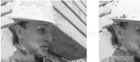
Figure 4.11. Visual comparison of the reconstructed 154th frame of Figure 4.10:(a) MQ-A and (b) SQ (q = 1) mapping cases.
A performance comparison of other simulation sets under adaptive WFQ is shown in Figure 4.12. The averages and deviations in PSNR, used as objective video quality metrics, are better in the case of adaptive WFQ than they are in static WFQ, as shown in Table 4.3. Also, the PSNRs of MQ mapping cases are better than those of SQ mapping cases with both static and adaptive WFQ packet-forwarding mechanisms, as shown in Table 4.3 and Figures 4.10, 4.12, and 4.13.
Figure 4.12. End-to-end video performance comparison with similar cost constraints under the adaptive WFQ. (a) MQ mapping (MQ-B) and SQ (q = 2). (b) MQ mapping (MQ-C) and SQ (q = 3).
Figure 4.13. End-to-end video performance comparison with similar cost constraints under static WFQ: (a) MQ mapping (MQ-A) and SQ (q = 1); and (b) MQ mapping (MQ-B) and SQ (q = 2), and (c) MQ mapping (MQ-C) and SQ (q = 3).
Table 4.3. Total Packet Loss Rate (%) And PSNR (dB) under Different Packet-Forwarding Mechanisms in the Same Case as Table 4.2
Mapping Set | Static WFQ | Adaptive WFQ | ||
|---|---|---|---|---|
Loss Rate (%) | PSNR (avg./dev.) | Loss Rate (%) | PSNR (avg./dev.) | |
SQ (q=1) | 9.87 | 21.9/3.38 | 9.55 | 23.3/3.40 |
MQ-A | 10.48 | 24.9/3.66 | 10.14 | 27.3/2.87 |
SQ(q=2) | 3.95 | 27.0/5.40 | 4.45 | 27.1/4.69 |
MQ-B | 4.39 | 30.4/3.66 | 5.12 | 30.8/3.24 |
SQ(q=3) | 2.80 | 28.5/3.39 | 3.26 | 28.5/3.99 |
MQ-C | 2.86 | 32.1/2.61 | 3.75 | 32.5/2.15 |
All conditions are the same as in Section 4.4.2, except for the restriction on multiple DS level mapping. Case (A) in Figure 4.4(a) represents a more delay-stringent, conversational application. It has a higher RDI and should be assigned only to AF2 and/or AF1. The delay-tolerant case (B) has lower RDI demand, as shown in Figure 4.4(a), and may be mapped to rather inexpensive queues such as AF2 and/or BE. The resulting mappings are denoted by MQ-B′ and MQ-A′ for Cases (A) and (B), respectively. Case (A) shows the comparison of SQ (q = 2) versus MQ-B′ (1,1,2,2,3,3,4,4,4,4), while Case (B) shows the comparison of SQ (q = 1) versus MQ-A′ (0,1,1,1,1,2,2,2,2,2). Note that they are using different total price budgets.
We expect the relatively delay-sensitive case (A) to achieve better delay/jitter performance than the corresponding SQ mapping set. And, the delay-tolerant case (B) should get better visual quality than SQ mapping at the cost of worse delay/jitter. Experimental results are shown in Table 4.4. In case A, we can see that MQ mapping gets better PSNR and better delay/jitter through RLI/RDI-aware QoS mapping. The perceptual video quality comparison between MQ and SQ mappings shows behavior similar to that of the MQ with RLI-only scenario. In case B, MQ mapping provides a similar benefit in average PSNR, although it suffers from more delay/jitters than SQ. Still, it is tolerable for this application. The detailed PSNR comparisons are shown in Figure 4.14.
Figure 4.14. End-to-end video performance comparison with RLI/RDI under adaptive WFQ: (a) MQ mapping (MQ-A′) and SQ (q = 1); and (b) MQ mapping (MQ-B′) and SQ (q = 2).
Table 4.4. Performance Comparison of Delay-Sensitive Applications (Case A) and Delay-Tolerant Applications (Case B)
Performance Parameters | Case A | Case B | ||
|---|---|---|---|---|
SQ Mapping (q = 2) | MQ-B′ | SQ Mapping (q = 1) | MQ-A′ | |
Total Budget Spent in Figure 4.3 | 2709 | 2667 | 1625 | 1521 |
Avg./Var. PSNR (dB) | 26.2/5.17 | 30.7/2.54 | 24.9/4.91 | 28.7/2.61 |
Avg. Total Loss Rate (%) | 3.39 | 3.47 | 4.96 | 5.28 |
Avg./Var. Delay (ms) | 98.4/21.60 | 89.6/20.45 | 103.1/18.78 | 121.7/30.72 |
The proposed adaptive packet-forwarding mechanism provides more persistent network DS levels regardless of network load fluctuation. A content-based video packet-forwarding mechanism was proposed to sustain effective QoS mapping between video applications and DiffServ-enabled networks in this chapter. This packet-forwarding mechanism was considered under both single- and multiple-queuing node systems. This mechanism is commonly used in all network nodes, but it still needs some intelligent functions for traffic conditioning at boundary regions of DiffServ-enabled network domains. If end-system adjustment with feedback as a closed-loop is combined with proposed open-loop QoS mapping, we can expect more persistent QoS mapping. This open-/closed-loop idea for QoS mapping control has been recently discussed in [115].
The next chapter will treat dynamic and aggregate QoS mapping, including feedforward and feedback QoS control at a special-purpose node that we call the CM gateway.
[1] Single/multiple queue scenarios are divided based on whether each network node has a physical or logical single/multiple class queue or not.