2.3. Feature Extraction
The power of a recognition system lies in the representation of pattern vectors because it is essential that the representation provide concise, invariant, and/or intelligible information on input patterns. Conversely, the applications intended also dictate the choice of representation. For example, in natural visual systems, it is known that images are preprocessed before being transmitted to the cortex [73]. Similarly, in image and vision analysis, raw image data must be preprocessed to extract vital characteristics (e.g., characteristics that are less dependent on imaging geometry and environment). As another example, in speech signal analysis, there is a wide variation in data rates, from 75bps for parametric text representation to 200,000bps for simple waveform representation [98].
2.3.1. Criteria of Feature Extraction
It is not easy to pinpoint an optimal representation strategy. The following offers some general criteria for the evaluation of feature representations.
Data compression. Only vital representations or features are extracted.
Invariance. The dependency of the features on environmental conditions should be minimized.
Ease of processing. A cost-effective hardware and software implementation should be feasible.
Other factors, such as overall cost, data rates, flexibility of representation, and quality of signals, should also be taken into account. In particular, data compression is an essential process in biometric identification. Depending on the data model, the following two approaches are often adopted to obtain highly compressed representations: (1) dimension reduction by projection onto vector subspace and (2) data clustering to simplify data representation. The subsequent section describes several dimension reduction methodologies. Comprehensive coverage of the data clustering strategy can be found in Chapter 3.
2.3.2. Projection Methods for Dimension Reduction
For convenience of analysis, high-dimensional input vectors are often first reduced into a set of linear combinations of the original raw vector. The reduced dimensionality of the subspace would facilitate many complex analysis tasks. There are two categories of subspace projection methods for dimensionality reduction: unsupervised and supervised.
Unsupervised subspace projection. Unsupervised projection methods have been widely used in many applications in which teacher values are not readily available. Data patterns can be projected into low-dimensional subspace according to either (1) their second-order moment or (2) their cluster separability. The former leads to the principal component analysis (PCA) approach while the latter leads to the independent component analysis (ICA) approach. PCA and ICA are arguably the most popular unsupervised subspace methods used in biometric applications [77,159].
Supervised subspace projection. For many classification applications, including face and speaker recognition, the training data consist of pairs of input/output patterns. In this case, it is more advantageous to adopt a supervised learning strategy to help determine the optimal projection. When class information is known, Fisher's discriminant criterion is commonly used to measure interclass separability. This leads to the so-called linear discriminant analysis (LDA) discussed in Section 4.2. Another supervised projection method very much worth pursuing is the well-known support vector machine (SVM), which is covered in detail in Chapter 4.
Principal Component Analysis
In statistics, a popular approach of extracting representation with maximum information is the principal component analysis (PCA). To retain the maximum amount of relevant information, the principal components (1) extract the most significant features that can best manifest the original patterns, and at the same time (2) avoid duplication or redundancy among the representations used.
Given an n-dimensional zero-mean wide-sense stationary vector process x(t) = [x1(t), x2(t), · · ·, xn(t)]T, then its autocorrelation matrix can be derived as
![]()
if the probability distribution function of {x(t)} is known a priori. The normalized eigenvectors of autocorrelation matrix Rx are {ei}, ||ei|| = 1, corresponding to the eigenvalues {λi}, where λ1 ≥ λ2 ≥ · · · λn ≥ 0. An eigen-component of a stochastic process x(t), ![]() , is its projection onto the one-dimensional subspace spanned by the eigenvector ei. The principal component of a signal is the first (and the largest) eigen-component
, is its projection onto the one-dimensional subspace spanned by the eigenvector ei. The principal component of a signal is the first (and the largest) eigen-component
![]()
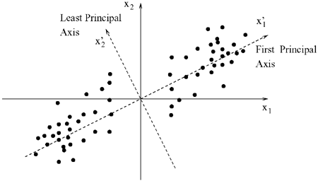
One such example is illustrated in Figure 2.5—the original pattern space is two-dimensional (n = 2) and the two principal axes for the pattern space are shown. Note that the first principal axis ![]() captures most of the distribution variance of the pattern space.
captures most of the distribution variance of the pattern space.
Figure 2.5. The  axis represents the principal component for the pattern space.

Given an n-dimensional vector process x(t) = [x1(t), x2(t), · · ·, xn(t)T, then any m-dimensional representation vector ![]() can be expressed as
can be expressed as
![]()
where W is an m×n matrix. Mathematically, the PCA is to find a matrix W such that an optimal estimate ![]() of x(t) can be reconstructed from x'(t) in terms of the mean-squared error. The solution W is formed by the first m eigenvector ei, i = 1, 2,..., m. In other words, the first m principal components are the eigen-components corresponding to the largest m eigenvalues: λi, i = 1, 2,..., m.
of x(t) can be reconstructed from x'(t) in terms of the mean-squared error. The solution W is formed by the first m eigenvector ei, i = 1, 2,..., m. In other words, the first m principal components are the eigen-components corresponding to the largest m eigenvalues: λi, i = 1, 2,..., m.
The PCA techniques have found many useful applications in signal and image filtering, restoration, pattern classification, and recognition. Specific application examples include biomedical signal processing, speech and image processing, antenna applications, seismic signal processing, geophysical exploration, data compression, high-resolution beam forming, separation of a desired signal from interfering waveforms (e.g., fetal ECGs from maternal ECGs), and noise cancelation [77,117,163,187,266]. It is worth mentioning that there are already widely available batch-processing methods—with very mature software developments (e.g., LIN-PACK and EISPACK)—for PCA or SVD computations.
Independent Component Analysis
In contrast to PCA, independent component analysis (ICA) extracts components with higher-order statistical independence. A common objective of PCA and ICA is to extract, say, m most representative linear features. The main difference lies in their selection criteria (i.e., PCA finds m uncorrelated expression profiles, while ICA finds m statistically independent expression profiles). Note that statistical independence is a stronger condition than uncorrelatedness [61, 159].
The kurtosis of a process y is defined as
![]()
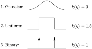
Figure 2.6 depicts the density functions and kurtosis values of three exemplifying processes: (a) a Gaussian random process has a kurtosis value of 3, (b) a uniformly distributed random process has a kurtosis value of 1.8, and (c) a binary-valued random process has a kurtosis value of 1. Note that the lower the kurtosis value, the more separable the data clusters become.
Figure 2.6. The density functions and corresponding kurtosis values for three random processes.

As noted before, the PCA and ICA use very different training criteria. The PCA maximizes the second-order covariance, while ICA minimizes the fourth-order kurtosis. A potentially advantageous feature of using ICA instead of PCA is that the kurtosis function k(y) is scale-invariant. (See Problem 1.)
The problem of finding the single most discriminative independent component can be mathematically formulated as follows: find a vector w such that y(t) = wTx(t) yields the minimum kurtosis:
Equation 2.3.1
![]()
Similarly, the full ICA problem is to find m linearly combined outputs, represented by a vector process y(t) = Wx(t) so that y(t) extracts the m most discriminative independent components. Here W is an m×n matrix formed by m independent row vectors wi, i = 1, 2,..., m, which can be extracted in a sequential manner—assuming that wi, i = 1, 2,..., m — 1 are already extracted and one is set to extract the m-th component. Mathematically, the vector wm can be found as the vector such that ![]() yields the minimum kurtosis under the orthogonality constraints that
yields the minimum kurtosis under the orthogonality constraints that ![]() = 0, i = 1, 2,..., m — 1. This constrained extraction scheme can be efficiently implemented via a popular numerical procedure known as the deflation technique. Indeed, the deflation method was incorporated into the KuicNet [189] originally designed for sequentially extracting independent components. (See Problem 2.)
= 0, i = 1, 2,..., m — 1. This constrained extraction scheme can be efficiently implemented via a popular numerical procedure known as the deflation technique. Indeed, the deflation method was incorporated into the KuicNet [189] originally designed for sequentially extracting independent components. (See Problem 2.)
2.3.3. Feature Selection
Sometimes, only a few selected features of a high-dimensional vector process would suffice for an intended classification task. For example, among many stocks listed on Hong Kong's stock market, only 33 are selected to calculate the Hang Seng index. This is because they are the most representative of different sectors and industries in Hong Kong. Note that unlike dimension reduction, there is no linear combination of features in the feature selection process.
The mathematical framework established previously can be applied to the preselection of features. Again, there are unsupervised and supervised preselection schemes.
Unsupervised preselection schemes. Following the same principle behind PCA, the second-order moment for each feature xi, i = 1,..., n reflects the extent of the pattern spread associated with that feature. The larger the second-order moment, the wider the spread, thus the more likely the feature xi contains useful information.
Given an n-dimensional zero-mean wide-sense stationary vector process x(t) = [x1(t), x2(t), …, xn(t)]T, then the feature or features with the highest variance will be selected. Mathematically, the feature index can be identified as:

Similarly, following the ICA-type argument, the fourth-order moment for each feature, xi, i = l,..., n, reflects how separable the data clusters are along that feature dimension. The lower the fourth-order moment, the more separable are the pattern clusters, thus the more likely it is that the feature contains useful information for the purpose of class discrimination.
Given an n-dimensional zero-mean wide-sense stationary vector process x(t) = [x1(t), x2(t), ···, xn (t)]T, then the feature(s) with the lowest kurtosis value will be selected. Mathematically, its index can be expressed as:

Supervised preselection schemes. If class information is known, a preselection method based on the Fisher discriminant analysis becomes very attractive. (Recall that the Fisher discriminant offers a convenient metric to measure the interclass separability embedded in each feature. ) Such a preselection approach entails computing Fisher's discriminant J(xi), i = 1,..., N, which represents the ratio of intercluster distance to intracluster variance for each dimension:
Equation 2.3.2

where μ1i and μ2i denote the means of the i-th feature xi for data belonging to C+ and C-, respectively. Similarly, σ1i and σ2i are the variances of the feature xi for data belonging to C+ and C_, respectively. The resulting values for each feature can then be used as a basis for feature selection. Ideally, the features selected will correspond to the index (or indices) i, which maximizes the contrast criterion J(xi). For an application example, see Zhang et al. [404].
2.3.4. Clustering Methods: Gaussian Mixture Models
From a clustering perspective, most biometric data cannot be adequately modeled by a single-cluster Gaussian model. However, they can often be accurately modeled via a Gaussian mixture model (GMM) (i.e., data distribution can be expressed as a mixture of multiple normal distributions.
To estimate the density parameters of a GMM statistic model, several prominent cluster estimation methods (e.g., the K-means or EM algorithms) can be adopted (see Chapter 3). In addition, the clustering task also requires the determination of an optimal number of clusters for the GMM. Such an optimal cluster number is often derived from well-known information theoretic metrics such as AIC or MDL—see [5, 313, 314]. The number of clusters is also tightly coupled with the cluster mass. The larger the number of clusters, the smaller the average cluster mass. From a practical perspective, the choice of cluster mass (and thus the number of clusters) depends heavily on the desired classification objectives—for example, whether the emphasis is placed on training accuracy or generalized performance.
Cluster-Then-Project versus Project-Then-Cluster
For high-dimensional or more complex data patterns, it is also advisable to pursue more sophisticated training strategies such as (1) cluster-then-project or (2) project-then-cluster methods.
As an example of the cluster-then-project approach, a projection aimed at separating two known classes, each modeled by a GMM, is proposed in Zhang et al. [404]. The proposed scheme makes use of both class membership information and intraclass cluster structure to determine the most desired projection for the purpose of discriminating the two classes.
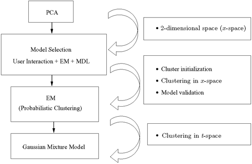
An example of the project-then-cluster approach is shown in the hierarchical clustering strategy depicted in Figure 2.7 [367, 370]. The following are three sub-tasks.
Project the data set from t-space onto a reduced-dimensional x-space, via say PCA.
Perform data clustering in the x-space.
Trace the membership information back to the t-space, and use the membership function as the initial condition and further fine-tune the GMM clustering by the EM algorithm in the t-space.
Figure 2.7. An illustration of the project-then-cluster approach. Projection of data from t-space to x-space, then after clustering in the lower-dimension subspace, trace the membership information back to the t-space.

