
5.6. Genetic Algorithm for Multi-Layer Networks
Another school of thought to train neural networks is to use an evolutionary search such as genetic algorithms [114, 243], evolutionary programming [100, 101], and evolution strategies [296, 325,338]. This section presents a hybrid algorithm that combines the standard RBF learning and genetic algorithms to find the parameters of RBF networks.
Unlike a local search, an evolutionary search maintains a population of potential solutions rather than a single solution. Therefore, the risk of getting stuck in local optima is smaller. Each candidate solution represents one neural network in which the weights can be encoded as a string of binary [71, 381, 383] or floating point numbers [119, 240, 283, 334]. The performance of each solution is determined by the network error function, which is to be optimized by evolutionary search. Because gradient information is not required, evolutionary search is applicable to problems where gradient information is unavailable or to cases where the search surface contains many plateaus. However, the iterative process in an evolutionary search requires evaluation of a large number of candidate solutions; consequently, evolutionary search is usually slower than local search. The lack of fine-tuning operations in evolutionary search also limits the accuracy of the final solution. The focus here is on genetic algorithms (one of the evolutionary search approaches).
5.6.1. Basic Elements of GAs
Evolutionary search maintains a population of candidate solutions for a given problem. In genetic algorithm (GA) terminology, the candidate solutions are called chromosomes. New chromosomes are generated by a set of genetic operators. Each chromosome is associated with a fitness value that reflects the solution quality (performance). Based on the fitness values, the population of chromosomes is maintained by selection and reproduction processes.
As introduced by Holland [137], each chromosome is comprised of a number of genes, each of which can take a binary value of 0 or 1. A mapping function is therefore required to decode the binary strings into corresponding solutions. The search space of all binary strings is the genotype space, and the decoded solutions constitute the phenotype space. Depending on the characteristics of the problem to be solved, the mapping function can be complex and nonlinear. Consequently, a simple search surface in a solution space might be represented by a complex and rugged search surface in a genotype space, which could hinder the search process [243]. While binary representations are common in boolean optimization problems [72, 316], many practitioners [68, 243] prefer to use problem-oriented representations. In particular, it is common to represent a chromosome as a string of floating point numbers [90,164]. With a problem-oriented representation, the correspondence between the genotype space and phenotype space is closer. This could reduce the complexity of the mapping function substantially.
5.6.2. Operation of GAs
As shown in Figure 5.8, the operation of the standard GA basically follows the structure of an evolutionary search. An initial population of size M is created by generating M chromosomes randomly. Based on the fitness values (f(ci), where i = 1, 2,. . . , M), some chromosomes with better performance are selected to form an intermediate population. For example, in the proportional selection process proposed by Holland, the probability of selecting a chromosome ck is determined by f(ck/∑i f (ci) (i.e., its fitness over the population's total fitness).
New chromosomes are generated from the selected chromosomes through genetic operations, where crossover and mutation operators are often used. In the standard GA proposed by Holland, each bit in a binary-encoded chromosome has a small probability of being flipped by mutation, and the crossover operator exchanges the binary substrings of two selected chromosomes to form new chromosomes. The M new chromosomes generated by the genetic operators constitute the new population for further processing. The iterative process is terminated when a satisfactory solution is found. It can also be terminated when the population has converged to a single solution. If the converged solution is an undesirable suboptimal solution, it is considered that premature convergence has occurred. Typically, premature convergence is a result of intense selection pressure (i.e., selection is heavily biased toward better-performing chromosomes) and insufficient exploration of search space [89, 204].
Figure 5.8. The procedure of the standard GA.
procedure GA

begin
     Initialize a population of M chromosomes ci, where i= 1,2, ...,M.
     Evaluate the fitness of every chromosome in the population.
     repeat
        Select some chromosomes in the population to form an intermediate
            population by means of a selection and reproduction mechanism.
        Generate new chromosomes from the intermediate population by means
            of a set of genetic operators.
        Evaluate the fitness of the new chromosomes.
        Create a new population of chromosomes to replace the old ones.
     until termination condition reached
endproc GA
|
5.6.3. Applications of GAs to Evolve Neural Networks
Many attempts to apply GAs to construct and train neural networks have been made—see Schaffer et al. [335], Whitley [380], and Vonk et al. [362] for comprehensive reviews. Typically, GAs are used to determine the network weights. For example, Montana and Davis [254] have successfully applied GAs to train feedforward neural networks for sonar data classification. Promising results have also been reported in other studies (e.g., [19, 70, 381]).
GAs can also be applied to determine an appropriate network architecture. For instance, Miller et al. [246] represented each chromosome as a matrix that defines the network connection (i.e., each entry in the matrix determines the existence of a connection). The network connection can also be represented by using a more abstract encoding scheme in which variable-length chromosomes are used to specify the connections [127].
In addition, GAs can be used to find a suitable training mechanism and its associated parameters. To this end, Chalmers [48] encoded the dynamics of a training procedure in a chromosome. In the GANNET system developed by Robbins et al. [315], some of the genes in the chromosomes were used to specify the learning rate and the momentum of the BP algorithm.
Another application that is not common in the field of neural networks is to use GAs for preprocessing and interpreting data. Typical examples include the selection of dominant features of input data [36, 49] and the selection of an appropriate training set [298]. Alternatively, GAs can be used to determine the input data patterns that produce a given network output [86].
Determination of RBF Centers by Genetic Algorithms
As mentioned in Section 5.4, the common approach to finding the parameters of RBF networks is to use unsupervised learning (e.g., the K-means algorithm and the K-nearest neighbor heuristic) to find the function centers and widths, and uses supervised learning (e.g., least-squares method) to determine output weights [255]. Although this approach is fast and a global minimum in output weight space is guaranteed to be found, the two-stage optimization process may lead to suboptimal solutions, especially when the K-means algorithm finds inappropriate function centers. An alternative approach is to replace the K-means algorithm with a genetic algorithm in an attempt to find the best locations for the function centers.
There are several approaches to embedding GA in the RBF training process. One approach uses space-filling curves to encode the function centers indirectly and evolve the parameters of the curves during the training process [378]. The success of this approach relies on the capability of the space-filling curves to capture the relevant properties of training data in the input space. Another approach evolves a population of genetic strings. Each of them encodes a single center and its associated width of an RBF network [379]. This method requires a shorter computation time as compared to the case where a single genetic string encodes the entire network. A more computation-intense, yet more powerful approach, is to evolve the centers, widths, and structure of the RBF networks simultaneously [26, 47]. It was found that this method is able to reduce the network complexity, which is particularly useful to the applications where runtime performance is an important issue.
This section describes a method that embeds a simple GA [114] into the RBF learning process. The result is referred to as the RBF-GA hybrid algorithm [224].[3] In the algorithm, each center of an RBF network is encoded as a binary string and the concatenation of the strings forms a chromosome. In each generation cycle, the simple GA is applied to find the center locations of the networks (chromosome), and the output weights are determined by a least-squares method. Therefore, the computation complexity of this approach falls between that of [378] and [26]. The proposed algorithm was applied to three artificial pattern classification problems to demonstrate that the best locations for the function centers may not necessarily be located inside the clusters of the training data.
[3] Hereafter, the networks trained with this algorithm are referred to as RBF-GA networks.
Embedding GA in RBF Learning
To implement the RBF-GA hybrid algorithm, the following items should be derived:
A fitness measure (performance evaluation)
A learning method for finding the output weights (RBF training)
A method for generating new genotypes from old ones (selection and reproduction)
Binary encoding is one of the common encoding methods for GAs because much of the existing GA theory is based on the assumption of fixed-length, fixed-order binary strings. This method can be classified into direct and indirect encoding [335]. For the former, little effort is required to decode the chromosome, and the transformation of genotypes into phenotypes is straightforward. The latter, on the other hand, requires more complicated decoding techniques.
Here, direct encoding is used to encode the function centers. Figure 5.9 shows the configuration of a binary string encoding m centers with each center being a point in an n-dimensional input space. Therefore, each chromosome is a concatenation of mn binary strings with each string being a 16-bit binary number. Each number is linearly mapped to a floating point number in [Umin, Umax]. In this work, Umin and Umax have been set to the minimum and maximum values of the training data in the input domain.
Figure 5.9. Structure of a chromosome

Fitness Measure
Training of neural networks usually involves the minimization of an objective function which, typically, is the mean-squared error (MSE) between the desired and actual outputs for the entire training set. However, GAs are usually applied to maximize a fitness function. Therefore, to apply GAs, a method is required to convert the objective function into a fitness function. A common approach is to use the transformation f(X) = l/(l + MSE(X)), where X denotes the training set and f the fitness function. Moreover, it is common practice to use the linear scaling
Equation 5.6.1
![]()
as suggested by Goldberg [114] to obtain the scaled fitness g(X). In this method, the values of a and b are chosen such that the scaled average fitness gav is equal to the average fitness fav, and the scaled maximum gmax is equal to a constant multiple of the average fitness (i.e., gmax = γfav). Therefore, after some mathematical manipulation, one has
Equation 5.6.2
![]()
To ensure that g(X) is always positive, check to see whether gmin(= afmin + b) is greater than 0. This leads to the following condition:
Equation 5.6.3
![]()
If Eq. 5.6.3 cannot be satisfied, set
Equation 5.6.4
![]()
so that gmin will be equal to 0. The scaling ensures that the individuals with scaled average fitness gav contribute one offspring on average during the selection process, while the best individual is expected to contribute a specified number (γ) of offspring. The advantage of this approach is that it can prevent individuals with small MSE (high fitness value) from dominating the population during the early stages of evolution. This can also improve selection resolution in the later stages of evolution when most individuals have high fitness values.
Selection and Reproduction
In this work, a simple genetic algorithm [114] has been used in the selection and reproduction processes. The operation of the simple GA is as follows. An initial population is created by randomizing the genetic strings. This is equivalent to randomizing the function centers of the corresponding RBF networks. In each generation, the algorithm creates a new population by selecting pairs of individuals from the current population and then allowing them to mate to produce new offspring. The new offspring are added to the new population. This process is continued until the size of the new population is the same as the current one. The evolution process is then repeated until a stopping criterion is met or the number of generations reaches a predefined maximum.
The roulette wheel selection method was used to pick an individual such that the fitter the individual, the higher the chance of selection for genetic operations. As a result, individual r has a probability pr of being selected, where
Equation 5.6.5

The RBF-GA Hybrid Algorithm
The RBF-GA hybrid algorithm consists of ten steps that follow.
1. | |
2. | Set generation t to 0. Randomize an initial population |
3. | Determine the value of Umax and Umin based on the maximum and minimum values of the training data in the input domain. |
4. | Set k = 1. Decode the chromosomes to form M networks and compute the width of each center according to the k-nearest-neighbor heuristic with K = 2. Find the output weights of each network using singular value decomposition (SVD) [285]. Find the best individual and denote it as |
5. | Evaluate the scaled fitness value of each individual |
6. | |
7. | Apply crossover to the two selected parents with probability pc to create two offspring. Next, apply mutation with probability pm to every bit of the two offspring. Then add the resulting chromosomes to the new population |
8. | k = k + 2. If k < M, go to Step 6; otherwise, go to Step 9. |
9. | |
10. | t = t + 1. If t < tmax, go to Step 4; otherwise stop. |
Experiments and Results
All experiments reported here were carried out on a SUN Sparc-10 workstation using a C++ genetic algorithm library (GAlib) [363]. The operation of the RBF-GA hybrid algorithm depends on the values of tmax, pc, pm, M, and γ. In the experiments, tmax = 100, pc = 0.6, pm = 0.01, M = 30, and γ = 1.2 have been set. These parameters typically interact with each other nonlinearly, and there are no conclusive results showing the best set of parameters. Therefore, the typical settings, which work well in other reports [249, 363], have been used.
Three problem sets, namely the XOR, overlapped Gaussian, and nonoverlapped Gaussian, have been investigated to evaluate the performance of the RBF-GA hybrid algorithm. For each problem, training of RBF networks using the K-means algorithm has also been performed so that comparisons can be made.
During the first experiments, a training set was created. The set consists of the input/output pairs {(x1, x2); y} such that y = r(x1) ε r(x2), where x1 and x2 belong to the set {0.0, 0.1, 0.2, 0.3, 0.7, 0.8, 0, 9, 1.0}, y ¤ {0.0,1.0}, and r(x) rounds the variable x to its nearest integer. The number of centers were set to four because there were four clusters in the input space. The effects of varying the number of centers were not investigated. Instead, the focus was on the differences in the performance of the RBF-GA hybrid and the standard RBF algorithms. Table 5.3 summarizes the MSE and training time (based on the CPU time of a SUN Sparc-10 workstation) of nine simulation runs of the two algorithms.
| Algorithm | MSE | Training Time |
|---|---|---|
| RBF-GA | 0.009 | 60 sec. |
| RBF | 0.089 | ≈ 1 sec. |
Table 5.3 shows that the MSE achieved by the RBF-GA hybrid algorithm is significantly smaller than that of the standard RBF learning algorithm. Figure 5.10 shows the locations of the function centers found by the RBF-GA hybrid algorithm and the K-means algorithm. One can deduce from this figure that the function centers found by the RBF-GA hybrid algorithm scatter around the input space, while most of the centers found by the K-means algorithm are located inside the input clusters. These results indicate that using the cluster centers as the function centers, as in standard RBF networks, may not necessarily give optimal performance.
Figure 5.10. Function centers found by the RBF-GA hybrid algorithm (+) and the K-means algorithm (‐).

Surprisingly, it was also noted that the networks trained by the RBF-GA hybrid algorithm provide high activation in the input space where no input data was present. This contrasts with the idea of using RBF networks with local perceptive fields in which networks are expected to produce low activation in regions without any training data. To further investigate this observation, two-dimensional Gaussian clusters were used in the experiments that followed.
In the second experiment, RBF networks were used to classify two overlapped Gaussian clusters into two classes. The mean vectors and covariance matrices of the two Gaussian clusters are shown in Table 5.4. The networks have two inputs, two function centers, and two outputs with each output corresponding to one class. The MSE, classification accuracy, and training time of the RBF-GA hybrid and the standard RBF algorithms are shown in Table 5.5.
| Cluster 1 (Class 1) | Cluster 2 (Class 2) | ||
|---|---|---|---|
| Mean vector | Cov. Matrix | Mean vector | Cov. Matrix |
 |  |  | |
| Algorithm | MSE | Classification Accuracy | Training Time |
|---|---|---|---|
| RBF-GA | 0.157 | 66.5% | 1814 sec. |
| RBF | 0.223 | 64.8% | 60 sec. |
Similar to the XOR problem, the MSE of the networks trained with the RBF-GA hybrid algorithm is lower than that of the standard RBF algorithm. This indicates that using the cluster centers found by the K-means algorithm can only provide a suboptimal solution. Figure 5.11 plots the decision boundaries, function centers, and the training data. A comparison between Figures 5.11(a) and 5.11(b) reveals that the decision boundary corresponding to the RBF-GA hybrid network is able to partially partition the two clusters—see the first quadrant of Figure 5.11(b)—resulting in a higher classification accuracy as shown in Table 5.5. This is because the GA is able to find appropriate locations for the function centers, which may not be located inside the input clusters. However, the function centers found by the K-means algorithm are always located inside the input clusters, as in Figure 5.11(a).
Figure 5.11. Decision boundaries and function centers found by (a) the standard RBF algorithm and (b) the RBF-GA hybrid algorithm. Note that in (b) only the centers and decision boundary of the best network were plotted.

Although the RBF-GA hybrid network gives a lower MSE and higher classification accuracy on the training data, it requires longer computation time for the population to converge. In the experiment, 1,000 two-dimensional data points for each cluster were used. The standard RBF algorithm took about one minute to train a network while the RBF-GA hybrid algorithm required 30 minutes. This is because there are 30 chromosomes in the population and, in each generation, the SVD algorithm must be applied 30 times in order to find the output weights of all individuals.
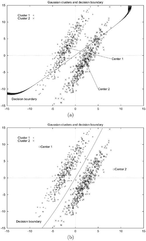
In the third experiment, two nonoverlapped Gaussian clusters with mean vectors and covariance matrices, as shown in Table 5.6, were classified by RBF networks with two function centers.
| Cluster 1 (Class 1) | Cluster 2 (Class 2) | ||
|---|---|---|---|
| Mean vector | Cov. matrix | Mean vector | Cov. matrix |
 |  |  |  |
The MSE, learning time, and classification accuracy are shown in Table 5.7, and Figure 5.12 shows the decision boundaries, function centers, and training data. Figure 5.12(b) demonstrates that the decision boundary formed by the RBF-GA hybrid network is able to separate the two clusters perfectly. On the other hand, the decision boundary created by the standard RBF network passes through both clusters, as shown in Figure 5.12(a). This leads to lower classification accuracy as shown in Table 5.7. The reason is that the RBF-GA hybrid algorithm considers all possible locations for the function centers in the input domain in order to minimize the MSE. Therefore, function centers outside the input clusters were found in this case, whereas function centers found by the K-means algorithm would always stay inside the Gaussian clusters.
Figure 5.12. Decision boundaries and function centers found by (a) the standard RBF algorithm and (b) the RBF-GA hybrid algorithm. Note that in (b) only the centers and decision boundary of the best network were plotted.
| Algorithm | MSE | Classification Accuracy | Training Time |
|---|---|---|---|
| RBF-GA | 0.021 | 100.0% | 1884 sec. |
| RBF | 0.075 | 89.5% | 60 sec. |
In conclusion, this subsection has described a hybrid algorithm, which combines the standard RBF learning and genetic algorithms, to find the parameters of RBF networks. Unlike the K-means algorithm, the RBF-GA hybrid algorithm is able to find the function centers outside the input clusters. The results demonstrate that, in some circumstances, the RBF networks with these center locations attain a higher recognition accuracy than that with centers located inside the input clusters.
Each generation of the RBF-GA hybrid requires the computation of the output weights of 30 networks and the evaluation of their fitness values. If the population takes many generations to evolve before an optimum is found, the hybrid algorithm will obviously require excessive training time. However, the main concern in practice is the runtime performance of the trained networks. Parallel implementation of GAs could be one possible solution to this problem.
In this work, only the locations of function centers are encoded in the genetic strings using direct binary encoding. The number of function centers (i.e., the network architecture) can also be evolved by GAs in future work. Moreover, local search methods, such as gradient descent, can be applied to fine-tune the center locations and the widths of basis functions during the course of Lamarckian evolution. This form of combining local search with GAs [185] could be applied to difficult problems where traditional RBF algorithms may fail to find a satisfactory solution.