To follow the examples in this tutorial you will need access to a workstation or space on a server system on which you can create a SQLite database.

You will also need the sqlite command-line tool to be installed and in your path. Full installation instructions can be found in Appendix A, “Downloading and Installing SQLite,” but for now the quickest way to get started is to use one of the precompiled sqlite binaries from http://www.hwaci.com/sw/sqlite/download.html.

Remember, SQLite writes its databases to the filesystem and does not require a database server to be running. The single executable sqlite (or sqlite.exe on Windows systems) is all that you need.

All of the code in this book is available for download on the Sams Publishing website at http://www.samspublishing.com/. Enter this book's ISBN (without the hyphens) in the Search box and click Search. When the book's title is displayed, click the title to go to a page where you can download the code to save you from retyping all the CREATE TABLE commands that follow. However, you don't have to download the sample database as we have included the full set of commands required for the tutorial in this book.

SQLite stores its databases in files, and you should specify the filename or path to the file when the sqlite utility is invoked. If the filename given does not exist, a new one is created; otherwise, you will connect to the database that you specified as the filename.

$ sqlite demodb
SQLite Version 2.8.12
Enter ".help" for instructions
sqlite>

Even without executing any SQLite commands, without any tables being created, connecting to a database as indicated in the preceding example will create an empty database file with the name specified on the command line.

$ ls –l
-rw-r--r--    1 chris    chris           0 Apr  1 12:00 demodb

No file extension is required or assigned by sqlite; the database file is created with the exact name specified. So how do we know that this is a SQLite database? You could opt for a consistent file extension, for example using somename.db (as long as .db is a unique extension for your system) or use a well-organized directory structure to separate your data from your program files.

When there is something inside your database, you can identify the file as a SQLite database by taking a look at the first few bytes using a binary-safe paging program such as less. The first line you will see will look like this:

** This file contains an SQLite 2.1 database **

We'll examine the format of the database file in more detail later in this chapter, but for now there's nothing more you need to know about creating and connecting to databases in SQLite. The CREATE DATABASE statement that you may be used to is not used.

The sample database is defined by a series of CREATE TABLE statements in a file called demodb.sql and there are some sample data records in sampledata.sql.

To execute the SQL in these files, use the .read command in sqlite.

$ sqlite demodb
SQLite version 2.8.12
Enter ".help" for instructions
sqlite> .read demodb.sql

Nothing will be displayed on screen unless there is an error in the SQL file—silence means that the commands were executed successfully.

It is also possible to execute an SQL file by redirecting it into sqlite from the command line, for instance:

$ sqlite demodb < sampledata.sql

As before, there will only be any output to screen if there are errors in the SQL file.

The sample database used in this tutorial is a very simple time-tracking system that might be used by a company to log employees' hours against client projects. There are five tables in the system, with the schema illustrated in Figure 2.1.

Figure 2.1. Schema of the sample database.

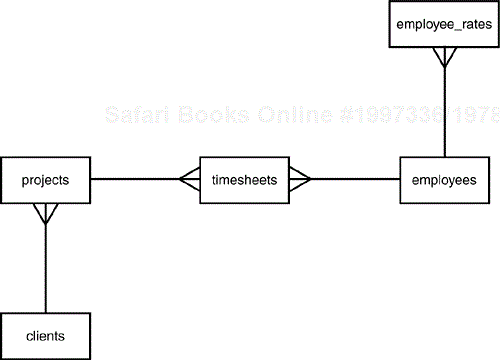
The tables holding employee and client details are very simple for this tutorial. In a real system the number of fields in these tables would be much higher, but for simplicity we've limited the employees and clients tables to just the basics.

CREATE TABLE employees (
  id INTEGER PRIMARY KEY,
  first_name CHAR NOT NULL,
  last_name CHAR NOT NULL,
  sex CHAR NOT NULL,
  email CHAR NOT NULL
);
CREATE TABLE clients (
  id INTEGER PRIMARY KEY,
  company_name CHAR,
  contact_name CHAR,
  telephone CHAR
);

Each table has an id field specified as INTEGER PRIMARY KEY, which we'll look at in more detail shortly. In a nutshell, this field is used to autogenerate a unique id number for each record added so that we don't have to.

Suppose that the company is working on, or has undertaken in the past, more than one job for each client and wants to keep the time spent on each project separate. To enable them to associate the hours on a timesheet with a particular project, we will create a projects table that looks like this:

CREATE TABLE projects (
  code CHAR PRIMARY KEY,
  client_id INTEGER NOT NULL,
  title CHAR NOT NULL,
  start_date INTEGER,
  due_date INTEGER
);

This time, rather than having SQLite assign our primary key, we've specified it as CHAR so that the company would assign its own project codes and employees would know the textual codes of the projects they are working on.

There is no direct relationship between employees and projects or clients—we have assumed that it is possible that any member of the workforce could be working on any of the current projects. Our timesheets table creates a link between projects and employees when they have done some work and records the date and how long they spent on that project.

CREATE TABLE timesheets (
  id INTEGER PRIMARY KEY,
  employee_id INTEGER NOT NULL,
  project_code CHAR NOT NULL,
  date_worked INTEGER NOT NULL,
  hours DECIMAL(5,2) NOT NULL
);

The final table, employee_rates, stores data on how much employees get paid. Rather than a single attribute in the employees table, this system allows us to remember the previous rates that an employee was paid before any raises were given. If we wanted to recalculate the cost of a project from some time ago, we would want to use the rates of pay in effect at the time and not the present ones.

CREATE TABLE employee_rates (
  employee_id INTEGER NOT NULL,
  rate DECIMAL(5,2),
  start_date INTEGER NOT NULL,
  end_date INTEGER
);

The way in which SQLite stores data is built upon the realization that strong typing of data, as found in virtually every RDBMS on the market, is actually not a useful thing. A database is designed to store and retrieve data, plain and simple, and as such the developer should not have to declare a column as numeric, textual, or binary, or tie it to any other specific data type. Needing to do so is a legacy weakness of the underlying system that had to be reflected in SQL, not a feature added to the language.

SQLite is “typeless.” It makes no difference whether you put a text string into an integer column or try to shove binary data into a text type. In fact you can—and should—specify the column types when each table is created. SQLite's SQL implementation allows you to do this, but it's actually ignored by the engine.

That said, it's still a good idea to include the column data types in your CREATE TABLE statements to help you think through the database design thoroughly and as a reminder to yourself and a hint to other programmers as to what your intended use of each column was. Suppose, also, that in the future you want to migrate or mirror your data onto an RDBMS that does require column typing—you'll be glad your table definitions are well documented.

You can always retrieve the CREATE TABLE statement used to create a table using the .schema command from within sqlite:

sqlite> .schema employees
CREATE TABLE employees (
  id INTEGER PRIMARY KEY,
  first_name CHAR NOT NULL,
  last_name CHAR NOT NULL,
  sex CHAR NOT NULL,
  email CHAR NOT NULL
);

In the demo database, all the data types were declared using familiar data type labels, but you may have noticed that we did not specify any lengths for the CHAR types, which would usually be required.

In fact the syntax of SQLite's CREATE TABLE statement specifies the column type attribute as optional. A valid column type is defined as any sequence of zero or more character strings (other than reserved words) optionally followed by one or two signed integers in parentheses.

Listing 2.1 shows a CREATE TABLE statement with some examples of ANSI SQL data types that are also valid in SQLite.

CREATE TABLE dummy (
  mychar CHAR(6),
  myvarchar VARCHAR(10)
  mydecimal DECIMAL(7,2),
  myinteger INTEGER,
  mytinyint TINYINT,
  myfloat FLOAT,
  mydate DATE
);

Listing 2.2 creates a table identical to the one in Listing 2.1, with imaginary column types to show that SQLite pays no attention to the actual types given.

CREATE TABLE dummy (
  mychar CHARACTER(6),
  myvarchar VARIABLE LENGTH CHARACTER
  mydecimal DECIMAL NUMBER(7,2),
  myinteger INT,
  mytinyint SMALL NUMBER,
  myfloat FLOATING POINT NUMBER,
  mydate CALENDAR DATE
);

Finally, Listing 2.3 shows that the same table can actually be created, if you are in a real hurry, without specifying any column types whatsoever.

CREATE TABLE dummy (
  mychar,
  myvarchar,
  mydecimal,
  myinteger,
  mytinyint,
  myfloat,
  mydate
);

You saw in the preceding section that the words that make up the name of a data type in the CREATE TABLE statement have no bearing on the data that can be stored in the table. There is actually one exception—if the column is defined exactly as INTEGER PRIMARY KEY, the value in the column must be a 32-bit signed integer; otherwise, an insert instruction will fail.

So why, with the decision that data typing was a bad idea, has SQLite implemented one column type that's different? The reason for an INTEGER PRIMARY KEY is to allow for the equivalent of an AUTOINCREMENT or IDENTITY column.

You can insert any 32-bit signed integer value into an INTEGER PRIMARY KEY column, or insert a NULL to tell SQLite to assign the value itself. Inserting a NULL will cause a value of one greater than the largest value already stored in that column to be used.

If the largest key value is already the maximum value that the column type allows—2^31–1, or 2147483647—then it's not possible to use a greater value for a new key. In this situation, SQLite picks a new key randomly.

We have used an INTEGER PRIMARY KEY called id on the employees, clients, and timesheets tables so that as new records are added, we do not need to assign this value ourselves.

In our sample tables, we have declared the date fields as INTEGER. Though SQLite has included some date and time functions since version 2.8.7, the typeless nature of SQLite does not provide a native storage format for dates. In our demo database tables, using an integer representation of the date serves our purposes well, for instance timesheets.date_worked is declared as INTEGER.

The SQLite date functions are based on a string date format, and we will examine them in detail in the next chapter.

Of course, SQLite will not enforce that the value stored in our (typeless) date columns must be an integer, but the use of INTEGER in the CREATE TABLE statement shows our intention for this field.

Using an integer date allows us to use one of two common formats. The UNIX timestamp format is the number of seconds since midnight on January 1, 1970 (known as the epoch), and a signed 32-bit integer is capable of storing dates up to 2037.

Some date calculations are made very easy using the timestamp format; for instance, to add one day to a value you just need to add 86400—the number of seconds in a day—to it. Most programming languages that SQLite can be embedded in work with this date format, and the SQLite date functions are also able to convert to and from a timestamp.

A more readable integer format is to present a date as YYYYMMDD (or YYYYMMDDHHIISS if the time is also required). It's much easier to see that 20040622 is June 22, 2004, than its equivalent timestamp value of 1322222400.

Although the YYYYMMDD format does not make date arithmetic possible without splitting up the individual components or converting to some other format, it can still be used for comparisons because an earlier date will always be represented as a lower integer value than a later date.

For our sample system, we are storing the dates that an employee worked and a due date for each project, so we might want to find out the hours worked in a particular month or how many projects are overdue, but we don't need to do any calculations and the time element is not required. Therefore, YYYYMMDD is a suitable date format for this system.

First of all, we'll add some employees and clients to the system.

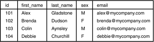
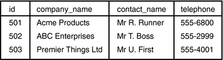
INSERT INTO employees (id, first_name, last_name, sex, email)
VALUES (101, 'Alex', 'Gladstone', 'M', '[email protected]'),

INSERT INTO employees (id, first_name, last_name, sex, email)
VALUES (102, 'Brenda', 'Dudson', 'F', '[email protected]'),

INSERT INTO employees (id, first_name, last_name, sex, email)
VALUES (103, 'Colin', 'Aynsley', 'M', '[email protected]'),

INSERT INTO employees (id, first_name, last_name, sex, email)
VALUES (104, 'Debbie', 'Churchill', 'F', '[email protected]'),

INSERT INTO clients (id, company_name, contact_name, telephone)
VALUES (501, 'Acme Products', 'Mr R. Runner', '555-6800'),

INSERT INTO clients (id, company_name, contact_name, telephone)
VALUES (502, 'ABC Enterprises', 'Mr T. Boss', '555-2999'),

INSERT INTO clients (id, company_name, contact_name, telephone)
VALUES (503, 'Premier Things Ltd', 'Mr U. First', '555-4001'),

Figures 2.2 and 2.3 show the contents of the employees and clients tables after this data has been loaded.

Figure 2.2. Contents of the employees table.

Figure 2.3. Contents of the clients table.

The sample data we have loaded specifies each id value explicitly so that, for instance, we can be sure that projects belong to the right client. However, if we add a new client to the system using the following statement, it will be given a new id of the next highest available number:

sqlite> INSERT INTO clients (company_name, contact_name, telephone)
   ...> VALUES ('Integer Primary Key Corp', 'Mr A. Increment', '555-1234'),

We don't have to go trawling through the data to find out what value SQLite assigned for the new primary key. The function last_insert_rowid() will return the integer value that was generated.

sqlite> select last_insert_rowid();
504

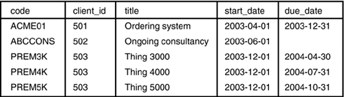
Next we'll insert details of the clients' projects. The due_date field is optional, and in the case of the second item in the following code being an ongoing project, we give it a NULL value.

INSERT INTO projects (code, client_id, title, start_date, due_date)
VALUES ('ACME01', 501, 'Ordering system', 20030401, 20031231);

INSERT INTO projects (code, client_id, title, start_date, due_date)
VALUES ('ABCCONS', 502, 'Ongoing consultancy', 20030601, NULL);

INSERT INTO projects (code, client_id, title, start_date, due_date)
VALUES ('PREM3K', 503, 'Thing 3000', 20031201, 20040430);

INSERT INTO projects (code, client_id, title, start_date, due_date)
VALUES ('PREM4K', 503, 'Thing 4000', 20031201, 20040731);

INSERT INTO projects (code, client_id, title, start_date, due_date)
VALUES ('PREM5K', 503, 'Thing 5000', 20031201, 20041031);

Figure 2.4 shows the contents of the projects table after these INSERT statements have been executed. Notice that the values in the client_id column correspond to records in the clients table, shown in Figure 2.3.

Figure 2.4. Contents of the projects table.

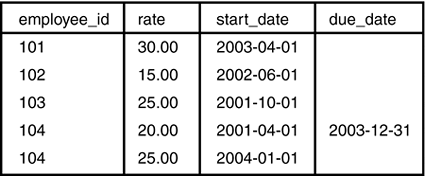
The following statements insert a rate of pay for each employee. The start_date is the date they joined the company and in most cases that rate is still in effect. We indicate that a rate is current by the end_date field being NULL.

Debbie Churchill, employee id 104, was given a raise, so there are two entries. Her hours worked before January 1, 2004, were paid at $20; from this date onwards she will be paid $25.

INSERT INTO employee_rates (employee_id, rate, start_date, end_date)
VALUES (101, 30.00, 20030401, NULL);

INSERT INTO employee_rates (employee_id, rate, start_date, end_date)
VALUES (102, 15.00, 20020601, NULL);

INSERT INTO employee_rates (employee_id, rate, start_date, end_date)
VALUES (103, 25.00, 20011001, NULL);

INSERT INTO employee_rates (employee_id, rate, start_date, end_date)
VALUES (104, 20.00, 20010401, 20031231);

INSERT INTO employee_rates (employee_id, rate, start_date, end_date)
VALUES (104, 25.00, 20040101, NULL);

Figure 2.5 shows the records inserted into the employee_rates table by the preceding statements. The employee_id column references records from the employees table—the values in this column correspond to the id column in Figure 2.2.

Figure 2.5. Contents of the employee_rates table.

Finally we have some timesheet information. This is only a small sample of information that might be in such a system where new data is added every day, but should be sufficient for demonstration purposes.

INSERT INTO timesheets (employee_id, project_code, date_worked, hours)
VALUES (101, 'ACME01', 20031229, 4);

INSERT INTO timesheets (employee_id, project_code, date_worked, hours)
VALUES (101, 'ABCCONS', 20031229, 2);

INSERT INTO timesheets (employee_id, project_code, date_worked, hours)
VALUES (101, 'PREM3K', 20040102, 6);

INSERT INTO timesheets (employee_id, project_code, date_worked, hours)
VALUES (102, 'ACME01', 20031229, 3);

INSERT INTO timesheets (employee_id, project_code, date_worked, hours)
VALUES (102, 'PREM4K', 20040102, 5);

INSERT INTO timesheets (employee_id, project_code, date_worked, hours)
VALUES (103, 'ABCCONS', 20031229, 2);

INSERT INTO timesheets (employee_id, project_code, date_worked, hours)
VALUES (103, 'PREM4K', 20040102, 3);

INSERT INTO timesheets (employee_id, project_code, date_worked, hours)
VALUES (103, 'ACME01', 20031229, 8);

INSERT INTO timesheets (employee_id, project_code, date_worked, hours)
VALUES (104, 'ACME01', 20040102, 8);

INSERT INTO timesheets (employee_id, project_code, date_worked, hours)
VALUES (104, 'ABCCONS', 20040102, 4);

Figure 2.6 shows the contents of the timesheets table after we have inserted this sample data. Notice that this table references two others, employees and clients—referenced by employee_id and project_code respectively.

Figure 2.6. The timesheets table after it has had the sample data inserted.

When you define a column as BLOB the column is still typeless, though as you saw earlier this does tell SQLite to use a text-based comparison when sorting on the field. SQLite is fully capable of storing binary data in any column, provided that there are no NUL (0x00, ASCII character zero) characters in the data.

As SQLite will store strings in its columns much more often than binary data, a NUL is the terminator for a variable-length character string and must be encoded somehow if it appears inside a piece of binary data.

Encoding can be done at the application level, for instance by encoding to base-64 or with URL-style encoding where NUL becomes its hex value represented as %00, and the percent character itself is encoded to %25.

SQLite also includes a pair of functions to encode and decode binary data, sqlite_encode_binary() and sqlite_decode_binary(). How binary data is encoded for any given column is an implementation choice left to the developer, so you can use supplied functions, adapt them from the sources in src/encode.c, or create your own.

Use SELECT to fetch rows from a table. Either use a comma-separated list of column names or use an asterisk to fetch all columns in the table.

sqlite> SELECT first_name, email FROM employees;
Alex|[email protected]
Brenda|[email protected]
Colin|[email protected]
Debbie|[email protected]

sqlite> SELECT * FROM clients;
501|Acme Products|Mr R. Runner|555-6800
502|ABC Enterprises|Mr T. Boss|555-2999
503|Premier Things Ltd|Mr U. First|555-4001

You'll notice that the format of the output isn't as readable as it could be. The sqlite program has a number of formatting options of which this mode, a pipe-separated list, is the default. The various output modes were discussed in Chapter 1, “Getting Started.”

Although character-separated output can be a useful format for parsing by a program, a tabulated output is clearer in print. Therefore, for the rest of this tutorial we will use column mode with headings turned on.

sqlite> .mode column
sqlite> .header on
sqlite> select * from clients;
id          company_name   contact_name  telephone
----------  -------------  ------------  ----------
501         Acme Products  Mr R. Runner  555-6800
502         ABC Enterpris  Mr T. Boss    555-2999
503         Premier Thing  Mr U. First   555-4001
504         Integer Prima  Mr A. Increm  555-1234

The values of company_name and contact_name in the preceding code are truncated. Their full values are stored in the database, but the column display format causes the output to be arbitrarily limited. You can specify the width settings in sqlite with the .width command:

sqlite> .mode column
sqlite> .width 4 24 15 10
sqlite> select * from clients;
id    company_name              contact_name     telephone
----  -----------------------   ---------------  ----------
501   Acme Products             Mr R. Runner     555-6800
502   ABC Enterprises           Mr T. Boss       555-2999
503   Premier Thing             Mr U. First      555-4001
504   Integer Primary Key Ltd   Mr A. Increment  555-1234

For the rest of this tutorial, display widths have been adjusted to suit the output and the actual .width commands issued are not shown in the code.

The WHERE statement specifies a conditional clause that can be used to restrict the dataset that is returned. To find all projects for Premier Things, we restrict the dataset on client_id.

sqlite> SELECT code, title
   ...> FROM projects
   ...> WHERE client_id = 503;
code        title
----------  ----------
PREM3K      Thing 3000
PREM4K      Thing 4000
PREM5K      Thing 5000

The AND and OR operators extend a WHERE condition logically. For instance, to find all projects for this client that were due on or before August 1, 2003, we could do the following:

sqlite> SELECT code, title, due_date
   ...> FROM projects
   ...> WHERE client_id = 503
   ...> AND due_date <= 20040801;
code        title       due_date
----------  ----------  ----------
PREM3K      Thing 3000  20040430
PREM4K      Thing 4000  20040731

You can use the BETWEEN operator to test if a value is in a given range. The following example finds all projects for Premier Things that were due during the month of July 2003.

sqlite> SELECT code, title, due_date
   ...> FROM projects
   ...> WHERE client_id = 503
   ...> AND due_date BETWEEN 20040701 AND 20040731;
code        title       due_date
----------  ----------  ----------
PREM4K      Thing 4000  20040731

You can use the IN operator to test if one value is in another given set of values. To select rows only where the value is not in the set, use NOT IN. The following example finds all projects for two specified clients:

sqlite> SELECT code, title
   ...> FROM projects
   ...> WHERE client_id in (501, 502);
code        title
----------  -------------------
ACME01      Ordering system
ABCCONS     Ongoing consultancy

We will look at the other relational operators that can be used in SQLite in Chapter 3, “SQLite Syntax and Use.” A full list can be found in Table 3.1.

The examples you have seen so far in this chapter all use integer values in the WHERE clause, and although SQLite is typeless, string values must still be enclosed in single quotes. The following are examples of some string comparisons:

sqlite> SELECT contact_name FROM clients
   ...> WHERE company_name = 'Acme Products';
contact_name
-------------
Mr R. Runner

Note that the equals operator for string comparisons is case sensitive. To find a case-insensitive match, use the LIKE operator. To test for inequality in strings, use != or NOT LIKE respectively.

sqlite> SELECT company_name FROM clients
   ...> WHERE company_name LIKE 'acME proDUCTs';
company_name
--------------
Acme Products

The LIKE operator can also be used to specify a substring search. The underscore character is used to represent any character, and a percent sign is a variable-length wildcard.

sqlite> SELECT company_name FROM clients
   ...> WHERE company_name LIKE 'A%';
company_name
---------------
Acme Products
ABC Enterprises

Table 2.1 shows some examples of wildcard matching using LIKE.

It is important to remember that NULL is a special value, actually meaning that an item has no value. It is not a zero value or an empty string, and comparing either of these values to NULL will always return false. Because NULL has no value, the equals operator cannot be used and you must test for NULL values using IS NULL.

To check whether a column value is NULL, use the IS NULL operator. The opposite, IS NOT NULL, will match any value including zero and an empty string. The following query finds all projects that are ongoing, that is with no due date:

sqlite> SELECT code, title FROM projects
   ...> WHERE due_date IS NULL;
code        title
----------  -------------------
ABCCONS     Ongoing consultancy

SQLite includes the function ifnull(), which can be used to specify an alternate to be used when a column value is NULL. For instance, we can visually indicate the ongoing projects in the database using this query:

sqlite> .mode column
sqlite> .header on
sqlite> SELECT code, ifnull(due_date, 'Ongoing')
   ...> FROM projects;
code        ifnull(due_date, 'Ongoing')
----------  ---------------------------
ACME01      20031231
ABCCONS     Ongoing
PREM3K      20040430
PREM4K      20040731
PREM5K      20041031

Likewise in a WHERE clause, we can select all the rates of pay that were current as of December 1, 2003, as in the following example:

sqlite> SELECT employee_id, rate
   ...> FROM employee_rates
   ...> WHERE start_date <= 20031201 
   ...> AND ifnull(end_date, 20031201) >= 20031201;
employee_id  rate
-----------  -----
101          30.00
102          15.00
103          25.00
104          20.00

The WHERE clause compares each start_date to see if the rate was valid on or before December 1, and checks that end_date falls on or after this date. For a row where end_date is NULL, the comparison is between 20031201 and 20031201, which will always be true.

Simple arithmetic functions in SQLite can be used in the column list of a SELECT statement or in the WHERE clause. In fact, to demonstrate the basic functions you don't even need to select from a table.

sqlite> SELECT 2 + 2;
2 + 2
----------
4

sqlite> SELECT 10 - 7;
10 - 7
----------
3

sqlite> SELECT 6 * 3;
6 * 3
----------
18

sqlite> SELECT 100 / 30;
100 / 30
----------
3

Note in the division example that a rounded integer is returned. To specify that you want a floating-point result, one of the arguments must be a float itself.

sqlite> SELECT 100.0 / 30;
100.0 / 30
----------------
3.33333333333333

The modulo operator is also supported, using the percent symbol, as in many other languages:

sqlite> SELECT 100 % 30;
100 % 30
----------
10

You can apply such operators to a selected column in the SELECT statement. For instance, to find all the current rates of pay plus 15%, we could do this:

sqlite> SELECT rate * 1.15 FROM employee_rates
   ...> WHERE end_date IS NULL;
rate * 1.15
-----------
34.5
17.25
28.75
28.75

Table 2.2 lists the arithmetic operators.

SQLite's concatenation operator is ||, which can be used to join two or more strings together.

sqlite> SELECT last_name || ', ' || first_name
   ...> FROM employees;
last_name || ', ' || first_name
-------------------------------
Gladstone, Alex
Dudson, Brenda
Aynsley, Colin
Churchill, Debbie

A number of built-in functions are also available for string manipulation. length() takes a single string parameter and returns its length in characters:

sqlite> SELECT company_name, length(company_name)
   ...> FROM clients;
company_name              length(company_name)
------------------------  --------------------
Acme Products             13
ABC Enterprises           15
Premier Things Ltd        18
Integer Primary Key Corp  24

To extract a section of a string, use substr(). Three parameters are required—the string itself, the start position (using 1 for the leftmost character), and a length:

sqlite> SELECT last_name, substr(last_name, 2, 4)
   ...> FROM employees;
last_name   substr(last_name, 2, 4)
----------  -----------------------
Gladstone   lads
Dudson      udso
Aynsley     ynsl
Churchill   hurc

To capitalize a string or convert it to lowercase, use upper() and lower() respectively:

sqlite> SELECT company_name, upper(company_name)
   ...> FROM clients;
company_name              upper(company_name)
------------------------  -------------------
Acme Products             ACME PRODUCTS
ABC Enterprises           ABC ENTERPRISES
Premier Things Ltd        PREMIER THINGS LTD
Integer Primary Key Corp  INTEGER PRIMARY KEY

One of SQLite's powerful features is the ability to add user-defined functions to the SQL command set. We will see how this is done using the various language APIs in Part II, “Using SQLite Programming Interfaces,” of this book.

The key concept of a relational database structure is that of separating your data into tables that model, generally speaking, separate physical or logical entities—the process of normalization—and rejoining them in a proper manner when executing a query.

In our sample database, we have tables containing a number of relationships. For instance, each employee has worked a number of hours, usually over the course of a number of days. The number of hours worked on each day is stored as a separate entry in the timesheets table.

The employee_id field in timesheets (often written as timesheets.employee_id) relates to the id field in employees (employees.id). To correlate each row of timesheet data with its respective employees record, we need to perform a join on these fields. In SQLite, this is how this looks:

sqlite> SELECT first_name, last_name, date_worked, hours
   ...> FROM employees, timesheets
   ...> WHERE employees.id = timesheets.employee_id;
first_name  last_name   date_worked  hours
----------  ----------  -----------  -----
Alex        Gladstone   20031229     4
Alex        Gladstone   20031229     2
Alex        Gladstone   20040102     6
Brenda      Dudson      20031229     3
Brenda      Dudson      20040102     5
Colin       Aynsley     20031229     2
Colin       Aynsley     20040102     3
Colin       Aynsley     20031229     8
Debbie      Churchill   20040102     8
Debbie      Churchill   20040102     4

The repeated information is the reason we split these tables up in the first place. Rather than store each name and any other employee details in the timesheets table, if we split off the employees data we only need to keep one copy.

In reality many more hours will be logged than in our example. So, supposing Brenda Dudson married and changed her name, we would have to update the last_name field for every row in timesheets. With the normalized relationship between the tables, only one data item needs to be changed.

In the preceding example we had to use employees.id to qualify that the join was to the id field in the employees table—timesheets also has a field named id. Using tablename.fieldname is the way to specify exactly which field you are talking about. If this were left out, SQLite would throw an error rather than attempt to make the decision for you:

sqlite> SELECT first_name, last_name, date_worked, hours
   ...> FROM employees, timesheets
   ...> WHERE id = employee_id;
SQL error: ambiguous column name: id

Notice that our selected columns were not qualified in this way. When the column name is unique across all the tables in a query, this is fine. If we wanted to fetch both id fields, though, they would need qualifying the same way.

To save typing the table name in full repeatedly whenever a column name has to be qualified, you can specify a table alias immediately after each table name in the FROM section. The following example aliases employees to e and timesheets to t, and the single-letter aliases are then used to specify which id fields are referenced in the selected columns list and WHERE clause.

sqlite> SELECT e.id, first_name, last_name, t.id, date_worked, hours
   ...> FROM employees e, timesheets t
   ...> WHERE e.id = t.employee_id;
e.id  first_name  last_name   t.id  date_worked  hours
----  ----------  ----------  ----  -----------  -----
101   Alex        Gladstone   1     20031229     4
101   Alex        Gladstone   2     20031229     2
101   Alex        Gladstone   3     20040102     6
102   Brenda      Dudson      4     20031229     3
102   Brenda      Dudson      5     20040102     5
103   Colin       Aynsley     6     20031229     2
103   Colin       Aynsley     7     20040102     3
103   Colin       Aynsley     8     20031229     8
104   Debbie      Churchill   9     20040102     8
104   Debbie      Churchill   10    20040102     4

A query can join many tables together, not just two. In the following example, we join employees, timesheets, projects, and clients to produce a report showing the title of all the projects and the names of all the employees that have worked on each one.

sqlite> SELECT c.company_name, p.title, e.first_name, e.last_name
   ...> FROM clients c, projects p, timesheets t, employees e
   ...> WHERE c.id = p.client_id
   ...> AND t.project_code = p.code
   ...> AND e.id = t.employee_id;
c.company_name      p.title               e.first_name  e.last_name
------------------  --------------------  ------------  ------------
Acme Products       Ordering system       Alex          Gladstone
Acme Products       Ordering system       Brenda        Dudson
Acme Products       Ordering system       Colin         Aynsley
Acme Products       Ordering system       Debbie        Churchill
ABC Enterprises     Ongoing consultancy   Alex          Gladstone
ABC Enterprises     Ongoing consultancy   Colin         Aynsley
ABC Enterprises     Ongoing consultancy   Debbie        Churchill
Premier Things Ltd  Thing 3000            Alex          Gladstone
Premier Things Ltd  Thing 4000            Brenda        Dudson
Premier Things Ltd  Thing 4000            Colin         Aynsley

Aggregate functions provide a quick way to find summary information about any of your data. The very simplest operation is a count, which is executed as follows:

sqlite> SELECT count(*) FROM employees;
count(*)
----------
4

The number of rows in the dataset is displayed. Of course this can be used in conjunction with a WHERE clause; for instance, we can see how many male employees there are.

sqlite> SELECT count(*) FROM employees
   ...> WHERE sex = 'M';
count(*)
----------
2

However, rather than executing one query for each possible value of sex, we can use a GROUP BY clause and an aggregate function to show us the number of employees of each sex.

sqlite> SELECT sex, count(*)
   ...> FROM employees
   ...> GROUP BY sex;
sex         count(*)
----------  ----------
F           2
M           2

Other aggregate functions available include sum(), avg(), min(), and max(), which find, respectively, the sum and average of a set of integers and the largest and smallest values from the set.

To find the average current hourly rate paid, we could use avg() as follows:

sqlite> SELECT avg(rate) FROM employee_rates
   ...> WHERE end_date IS NULL;
avg(rate)
----------
23.75

To find the averages for men and women, we would include sex in the column list, and then use the GROUP BY clause on this column.

sqlite> SELECT sex, avg(rate)
   ...> FROM employees e, employee_rates r
   ...> WHERE e.id = r.employee_id
   ...> GROUP BY sex;
sex         avg(rate)
----------  ----------
F           20
M           27.5

We'll see in Part II of this book how you can create your own aggregating functions using the language APIs that SQLite provides.

Unless it is specified, the order in which selected rows are returned is undefined—though they are usually brought back in the order in which they were inserted. SQLite uses the ORDER BY clause to specify the ordering of a dataset.

We actually inserted our employees in order of first name, but if we want the result of our SELECT statement to sort on last_name, we can add this in an ORDER BY clause:

sqlite> SELECT last_name, first_name
   ...> FROM employees
   ...> ORDER BY last_name;
last_name   first_name
----------  ----------
Aynsley     Colin
Churchill   Debbie
Dudson      Brenda
Gladstone   Alex

The ORDER BY can specify more than one column for sorting. Note that the columns listed need not actually appear in the list of columns selected. In the following example we order by sex first, then by last_name. The two women appear at the top of the list in alphabetical order, followed by the men.

sqlite> SELECT last_name, first_name
   ...> FROM employees
   ...> ORDER BY sex, last_name;
last_name   first_name
----------  ----------
Churchill   Debbie
Dudson      Brenda
Aynsley     Colin
Gladstone   Alex

The ORDER BY clause is one situation where the data type of the columns referenced actually does matter, because SQLite needs to make a decision on how to evaluate a comparison between two values.

For instance if a column does not have a data type, what determines whether a value of 100 is higher or lower than a value of 50? As two integers, clearly 100 is higher that 50, but a string comparison would consider 50 “higher” because its first character appears later in the ASCII character set.

In earlier versions of SQLite (version 2.6.3 and below), all comparisons for sorting were treated as numeric, with strings being compared alphabetically only if they could not be evaluated as numbers. Since version 2.7.0, a column will take one of two types, either numeric or text, and the CREATE TABLE statement actually determines which type is used.

Don't be confused—a numeric column type is still typeless inasmuch as it can store any kind of data, so it is not restricted to integer, as an INTEGER PRIMARY KEY is, or indeed to any other numeric type. The fact that a column is considered numeric only comes into play when a value has to be compared.

You saw before that any number of names can make up a data type name in the CREATE TABLE statement. If the name contains one or more of the following strings, the column will be declared text. For all other data type names, or if the data type is omitted, it will be numeric.

To confirm the data type of a column you can use the typeof() function. Because the function would apply to the entire dataset, limit the records returned using LIMIT.

sqlite> SELECT typeof(code), typeof(client_id)
   ...> FROM projects
   ...> LIMIT 1;
typeof(code)  typeof(client_id)
------------  -----------------
text          numeric

Expressions also have an implicit data type for comparisons, usually determined by the outermost operator regardless of the actual arguments. An arithmetic operator returns a numeric result and a string operator returns a text result, regardless of the implied types of the arguments themselves.

As you might expect, you can also check the data type of an expression using typeof():

sqlite> select 123 + 456, typeof(123 + 456);
123 + 456   typeof(123 + 456)
----------  ------------------------
579         numeric

sqlite> select 123 || 456, typeof (123 || 456);
123 || 456  typeof (123 || 456)
----------  ------------------------
123456      text

sqlite> select 'abc' + 456, typeof('abc' + 456);
'abc' + 1   typeof('abc' + 456)
----------  ------------------------
456         numeric

Although this problem does not occur with our demo database, sometimes a query will return more rows than you want to process. You can use the LIMIT clause to limit the number of rows returned by specifying a number:

sqlite> SELECT * FROM employees LIMIT 2;
id    first_name  last_name   sex  email
----  ----------  ----------  ---  --------------------
101   Alex        Gladstone   M    [email protected]
102   Brenda      Dudson      F    [email protected]

LIMIT can be used in conjunction with a WHERE clause to further restrict the dataset after any conditions have been evaluated. Any ORDER BY clause specified is also taken into account first before limiting takes place. The following example fetches only the first record alphabetically from all the male employees.

sqlite> SELECT * FROM employees
   ...> WHERE sex = 'M'
   ...> ORDER by last_name, first_name
   ...> LIMIT 1;
id    first_name  last_name   sex  email
----  ----------  ----------  ---  --------------------
103   Colin       Aynsley     M    [email protected]

LIMIT optionally takes an offset parameter, so that rather than returning the first N rows, it will skip a number of rows from the top of the dataset and then return the next N rows. In the following example, rows 3 and 4 are returned from the query, using an offset of 2 and a limit of 2.

sqlite> SELECT * FROM projects
   ...> ORDER BY due_date DESC
   ...> LIMIT 2, 2;
code      client_id   title            start_date  due_date
--------  ----------  ---------------  ----------  ----------
PREM3K    503         Thing 3000       20031201    20040430
ACME01    501         Ordering system  20030401    20031231

To modify records in your database or remove them, use the SQL commands UPDATE and DELETE. Both use a WHERE clause to specify which rows are affected, so the syntax will be fairly familiar to you by now.

Suppose we want to split some of the hours worked on the Ongoing Consultancy project for ABC Enterprises off into another project. The UPDATE statement would look something like this:

UPDATE timesheets
SET project_code = new_project_code
WHERE condition

Let's follow this example through and move all the hours spent in 2003 into a new project code ABC2003. First we insert a new project record.

sqlite> INSERT INTO projects (code, client_id, title, start_date, due_date)
   ...> VALUES ('ABC2003', 502, 'Work in 2003', 20030101, 20031231);

Then we can run an UPDATE command to move all the 2003 hours to this new project.

sqlite> UPDATE timesheets
   ...> SET project_code = 'ABC2003'
   ...> WHERE project_code = 'ABCCONS'
   ...> AND date_worked BETWEEN 20030101 and 20031231;

The UPDATE is silent unless there is a problem, so there is no confirmation on screen. The following query to find the total number of hours worked on each project and the extent of the work dates can be used to show that the update has indeed taken place.

sqlite> SELECT project_code, count(*), min(date_worked), max(date_worked)
   ...> FROM timesheets
   ...> GROUP BY project_code;
project_code  count(*)  min(date_worked)  max(date_worked)
------------  --------  ----------------  ----------------
PREM4K        2         20040102          20040102
PREM3K        1         20040102          20040102
ABCCONS       1         20040102          20040102
ABC2003       2         20031229          20031229
ACME01        4         20031229          20040102

You can update multiple columns in one UPDATE statement by supplying a comma-separated list of assignments. For instance, to update the contact name and telephone number for a client in one statement, you could do the following:

sqlite> UPDATE clients
   ...> SET contact_name = 'Mr A. Newman',
   ...>     telephone = '555-8888'
   ...> WHERE id = 501;

Let's say you change your mind about the previous reallocation of timesheets and want to remove project code ABC2003. The DELETE syntax for this reads as you might expect:

sqlite> DELETE FROM projects
   ...> WHERE code = 'ABC2003';

A list of columns is not required for a DELETE because action is taken on a record-by-record basis. Asking SQLite to delete only a particular column makes no sense. To blank the values of specific columns while keeping the record in the database, use an UPDATE and set the necessary fields to NULL.

The DELETE we did in the preceding section has actually left our data in quite a mess. The relationship between timesheets and projects is broken because we now have timesheet data with a nonexistent project_code.

Some database systems have a cascading delete facility, which means that when a FOREIGN KEY is defined on a table, if that key value is deleted from the master table, the corresponding child records are also deleted. SQLite does not support this functionality in the same way, although we will look at a way it can be implemented with a trigger in the next chapter.

However, now that we are in this situation, we can use it to demonstrate the LEFT JOIN operator in SQLite. The joins you saw previously used a WHERE clause to specify the relationship between the tables, for instance timesheets.project_code = projects.code.

A LEFT JOIN also uses a condition to combine the data from both the tables, but where a row from the first table does not have a corresponding row in the second, a record is still returned—containing NULL values for each of the fields in the second table.

Let's see this in action. The following query specifies a LEFT JOIN between timesheets and projects so that our orphaned timesheet records still appear, but with blank project information.

sqlite> SELECT p.title, p.code, sum(t.hours)
   ...> FROM timesheets t
   ...> LEFT JOIN projects p
   ...> ON p.code = t.project_code
   ...> GROUP BY p.title, p.code
   ...> ORDER BY p.title;
p.title                   p.code    sum(t.hours)
------------------------  --------  ------------
                                    4
Ongoing consultancy       ABCCONS   4
Ordering system           ACME01    23
Thing 3000                PREM3K    6
Thing 4000                PREM4K    8

So to find details of the timesheet entries that do not have a matching project code, we can modify the preceding query and use an IS NULL condition to take advantage of this property of a LEFT JOIN.

sqlite> SELECT t.*
   ...> FROM timesheets t
   ...> LEFT JOIN projects p
   ...> ON p.code = t.project_code
   ...> WHERE p.code IS NULL;
t.id  t.employee_id  t.project_code  t.date_worked   t.hours
----  -------------  --------------  --------------  --------
2     101            ABC2003         20031229        2
6     103            ABC2003         20031229        2

There is another, often more readable, way to perform the same timesheet query using a nested subquery. SQLite allows you to use the dataset produced by any query as the argument to an IN or NOT IN expression.

The following query finds all the timesheet records where the project code is not one of those in the projects table.

sqlite> SELECT *
   ...> FROM timesheets
   ...> WHERE project_code NOT IN (
   ...>   SELECT code
   ...>   FROM projects
   ...> );
id    employee_id   project_code    date_worked     hours
----  ------------  --------------  --------------  --------
2     101           ABC2003         20031229        2
6     103           ABC2003         20031229        2

Though more readable, the NOT IN query in this example is usually less efficient than the LEFT JOIN method. We will deal with query optimization in more detail in Chapter 4, “Query Optimization.”

Another type of join possible in SQLite is the Cartesian join. This is something that usually only happens by mistake, so we mention it here only so that you are able to spot such problems.

If two (or more) tables are selected without a proper join in the WHERE clause, every row in table 1 is paired with each row in table 2 to produce a Cartesian product—the number of rows returned is the product of the number of rows in each table.

The following query shows a Cartesian join on the clients and projects tables, and you should be able to see that with tables containing significant amounts of data, a Cartesian join is generally not a desirable result.

sqlite> SELECT c.company_name, p.title
   ...> FROM clients c, projects p;
c.company_name            p.title
------------------------  ------------------------
Acme Products             Ordering system
Acme Products             Ongoing consultancy
Acme Products             Thing 3000
Acme Products             Thing 4000
Acme Products             Thing 5000
ABC Enterprises           Ordering system
ABC Enterprises           Ongoing consultancy
ABC Enterprises           Thing 3000
ABC Enterprises           Thing 4000
ABC Enterprises           Thing 5000
Premier Things Ltd        Ordering system
Premier Things Ltd        Ongoing consultancy
Premier Things Ltd        Thing 3000
Premier Things Ltd        Thing 4000
Premier Things Ltd        Thing 5000
Integer Primary Key Corp  Ordering system
Integer Primary Key Corp  Ongoing consultancy
Integer Primary Key Corp  Thing 3000
Integer Primary Key Corp  Thing 4000
Integer Primary Key Corp  Thing 5000

Transactions are the way that databases implement atomicity—the assurance that the entirety of a request to alter the database is acted upon and not just part of it. Atomicity is one of the key requirements of a mission-critical database system.

Every time the database is changed—in other words for any INSERT, UPDATE, or DELETE to take place—the change must take place inside a transaction. SQLite will start an implicit transaction whenever one of these commands is issued if there is not already a transaction in progress.

You would want to start a transaction explicitly if you wanted to make a series of changes that must all take place at the same time. Simply issuing the commands one after each other does not absolutely guarantee that if the earlier commands are executed the later commands will also have been processed.

Let's say in our demo database that we wanted to change one of the project codes, and because the timesheets table is joined to projects on project_code, we need to ensure that the same change is made to both tables at the same time. In SQLite we do this as follows:

sqlite> BEGIN TRANSACTION;
sqlite> UPDATE projects
   ...> SET code = 'ACMENEW'
   ...> WHERE code = 'ACME01';
sqlite> UPDATE timesheets
   ...> SET project_code = 'ACMENEW'
   ...> WHERE project_code = 'ACME01';
sqlite> COMMIT TRANSACTION;

Until the COMMIT TRANSACTION command is issued, neither of the UPDATE statements have caused a change to be made to the database. A query executed within the transaction will consider these changes to have been made; however, the ROLLBACK TRANSACTION command can be used to cancel the entire transaction. The following example shows a mistake made when making an update that was rolled back:

sqlite> BEGIN TRANSACTION;
sqlite> UPDATE clients
   ...> SET contact_name = 'Mr S. Error';
sqlite> SELECT * from clients;
id    company_name              contact_name    telephone
----  ------------------------  --------------  ----------
501   Acme Products             Mr S. Error     555-8888
502   ABC Enterprises           Mr S. Error     555-2999
503   Premier Things Ltd        Mr S. Error     555-4001
504   Integer Primary Key Corp  Mr S. Error     555-1234
sqlite> ROLLBACK TRANSACTION;
sqlite> SELECT * from clients;
id    company_name              contact_name     telephone
----  ------------------------  ---------------  ----------
501   Acme Products             Mr A. Newman     555-8888
502   ABC Enterprises           Mr T. Boss       555-2999
503   Premier Things Ltd        Mr U. First      555-4001
504   Integer Primary Key Corp  Mr A. Increment  555-1234

You've already seen that from the sqlite tool you can view the list of tables in a database with the .tables command and view the schema of any table using .schema.

However, SQLite is designed as an embedded database, and ultimately you will be writing applications in your language of choice and calling SQLite API functions where the commands beginning with a period that are available in sqlite cannot be invoked directly.

We finish this chapter by looking at the internal tables that can be used to query a database and its table schemas.

The master table holding the key information about your database tables is called sqlite_master, and using sqlite you can see its schema as you might expect:

sqlite> .schema sqlite_master
CREATE TABLE sqlite_master (
  type text,
  name text,
  tbl_name text,
  rootpage integer,
  sql text
);

The type field tells us what kind of object we are dealing with. So far we've only looked at tables, but indexes and triggers are also stored in sqlite_master, and we'll look at these in more detail in Chapter 3.

For a table, name and tbl_name are the same. An index or trigger will have its own identifier, but tbl_name will contain the name of the table to which it applies. The sql field contains the CREATE TABLE (or CREATE INDEX or CREATE TRIGGER) statement issued when each database object was created.

So, to find the names of all tables in a database, do the following:

sqlite> SELECT tbl_name
   ...> FROM sqlite_master
   ...> WHERE type = 'table';
tbl_name
--------------------
employees
employee_rates
clients
projects
timesheets

Or to find the SQL command used to create a table, the following query will work—shown here in line output mode so that you can see the whole text.

sqlite> SELECT sql
   ...> FROM sqlite_master
   ...> WHERE type = 'table'
   ...> AND tbl_name = 'projects';
  sql = CREATE TABLE projects (
  code CHAR PRIMARY KEY,
  client_id INTEGER NOT NULL,
  title CHAR NOT NULL,
  start_date INTEGER,
  due_date INTEGER
)