Search in book...
Toggle Font Controls
Create new playlist

Name your new playlist

Playlist description (optional)
Sign In

Email address

Password

Forgot Password?

or

Continue with Facebook

Continue with Google
Sign Up

Full Name

Email address

Confirm Email Address

Password

or

Continue with Facebook

Continue with Google

Chapter 3

Air

Abstract

In this chapter the use of air as a raw material for the production of the species that constitute the mixture, oxygen, nitrogen, and noble gases is shown, as well as its use as a comburant. Air liquefaction and separation technologies are described and analyzed using unit operation principles. In addition to the classic approach using diagrams and shortcut methods, process simulators (eg, CHEMCAD) are used to perform calculations and compared. Various liquefaction cycles—such as Linde’s, Claude’s, and Phillips’s, and air separation technologies including the operation of Linde’s double column—are evaluated. Moreover, air typically carries a certain level of humidity that affects its use as a refrigerant in cooling towers, and as a comburant and raw material. Air moisture characterization and its desiccation are evaluated over a number of examples.

Keywords

Air; oxygen; nitrogen; air separation; air liquefaction; moisture

3.1 Introduction

3.1.1 Composition

Air is a plentiful raw material. Its composition includes nitrogen, oxygen, and noble gases (such as argon). Technically, air is assumed to have a composition of 79% nitrogen and 21% oxygen, as well as the moisture corresponding to the weather conditions. A more detailed composition can be found in Table 3.1. This composition can be altered by electric discharges so that certain molecules (such as H₂O, N₂, O₂, and CO₂) are dissociated and others formed (such as C₂H₂, H₂O₂, O₃, HNO₃, NH₃, NH₄NO₃, and NH₄OH). These species can be used as nitrogen fertilizer when it rains, but it is not enough to cover all needs.

Table 3.1

Air Composition

Chemical	Volume Fraction	Mass Fraction
Nitrogen	78.14	75.6
Oxygen	20.92	23.1
Argon	0.94	0.3
Neon	1.5×10⁻³	1×10⁻³
Helium	5×10⁻⁴	0.7×10⁻⁴
Krypton	1×10⁻⁴	3×10⁻⁴
Hydrogen	5×10⁻⁵	0.35×10⁻⁵
Xenon	1×10⁻⁵	4×10⁻⁵

3.1.2 Uses

Air can be used as a comburant, as itself, or as a source of oxygen. The second main use is as a raw material for the production of N₂, O₂, and noble gases. Wastewater treatment is another alternative use. Air is bubbled in the pools of water treatment plants to decompose organics. Finally, it is possible, under the proper operating conditions, to produce NO as an intermediate in the production of HNO₃. For the production of NO we need high temperatures and fast cooling of the products. From NO, NO₂ is obtained via oxidation, and is later absorbed into water to produce HNO₃.

Nitrogen is a colorless, odorless, tasteless, nontoxic, and relatively inert gas. It does not sustain combustion or respiration, but it can react with metals such as lithium and magnesium to obtain nitrides. Furthermore, at high temperatures it combines with hydrogen, oxygen, and other elements. At atmospheric pressure, it condenses at 77.3K as a colorless liquid, and solidifies at 63.1K in the form of white crystals. As a cryogenic liquid, it is nonmagnetic and stable against mechanical shock.

It represents 78% of the atmosphere, but its weight contribution is small, 0.03% with respect to the mass of water and Earth. It can also be found as Chile saltpeter or Peru saltpeter. In order to use nitrogen in synthesis, purity over 99.8% is required. The main uses are the production of NH₃, CaCN₂, NaCN, or as an inert gas to pressurize aircraft tires, and purge pipelines, reactors, and storage tanks. As a liquid, it can be used to capture CO₂ and in medical applications (Hardenburger and Ennis, 1993; Häussinger, 1998).

Oxygen is a colorless, odorless, tasteless, nontoxic gas. At atmospheric pressure it condenses at 90.1K as a blue liquid, and solidifies at 54.1K to form blue crystals. It is less volatile than nitrogen and thus it is obtained from the bottom of air distillation columns.

It is the more abundant species, representing 50% of the atmosphere, water, and cortex weight. High purity oxygen (above 99.5%) is used in metal cutting and welding. Lower purity oxygen (85–99%) and enriched air (below 85%) can be used as oxidants, to produce C₂Ca, for the partial oxidation of methane to syngas, for the catalytic production of HNO₃ from ammonia, for the oxidation of HCl to Cl₂, or as a bleach in the production of paper. Oxygen supports life and is used in water treatment (Hansel, 1993; Kirschner, 1998).

Noble gases are typically used to fill light bulbs, fluorescent pipes, and electronic devices. For instance, argon is used in metal welding as an inert atmosphere. Helium can be used in stratospheric balloons and diving apparatuses.

3.2 Air Separation

3.2.1 History

For centuries air was considered a gas element. In 1754 Joseph Black identified what he called “fixed air” (CO₂), so-called because it could be returned, or fixed, into the sorts of solids from which it was produced. Later, in 1766 Henry Cavendish produced a highly flammable substance that was eventually named hydrogen by Lavoisier. The word has its roots in its Greek meaning, “water maker.” Finally, in 1772 Daniel Rutherford found that when he burned material in a bell jar, and then absorbed all the “fixed” air by soaking it up with a substance called potash, a gas remained. Rutherford referred to it as “noxious air” because it asphyxiated mice placed in the jar. This gas was what we today call nitrogen. The series of experiments culminated in 1774 when Joseph Priestley, inventor of carbonated water and the rubber eraser, found that “air is not an elementary substance, but a composition,” or mixture, of gases. Using a 12-inch-wide glass “burning lens,” he focused sunlight on a lump of reddish mercuric oxide in an inverted glass container placed in a pool of mercury. The gas emitted was “five or six times as good as common air.” In subsequent tests, it caused a flame to burn intensely and kept a mouse alive about four times as long as a similar quantity of air. Priestley called his discovery “dephlogisticated air” based on the theory that it supported combustion so well because it had no phlogiston in it, and hence could absorb the maximum amount during burning. It was the French chemist Antoine Lavoisier who coined the name “oxygen”(American Chemical Society, 1994).

From the discovery of the components of air, research on gases continued. A number of important dates highlight key developments in the processes to liquefy and separate the components of air. For instance, the Joule-Thompson (Kelvin) effect was discovered in 1853 when it was realized that a compressed gas cools down when it expands, typically 0.25°C per atmosphere. There are some exceptions, such as hydrogen. In 1863 the concept of critical temperature was defined as the temperature above which it is not possible to liquefy CO₂ by compression. In 1877 James Dewar, in Faraday’s laboratory, liquefied hydrogen. At the same time in Switzerland and France, oxygen was also liquefied. In our simplified review of history we reach 1895, when Karl von Linde proposed a procedure to liquefy air by isothermal compression followed by isobaric cooling and expansion. A number of modifications of this basic idea allowed higher yields.

3.2.2 Classification of Air Separation Methods

A Physical separation

• Cryogenic:

• Air distillation

• Noncryogenic:

• Adsorption on molecular sieves

• Diffusion across membranes

B Chemical separation

This consists of reacting one of the components so that it is fixed. In this case the most reactive component is the O₂, and thus we obtain oxygen combined as a product and N₂ as a byproduct.

3.2.2.1 Physical separation

3.2.2.1.1 Cryogenic methods: air liquefaction and distillation

In order to separate air via rectification, a part of it should be liquid. We can only do that below the critical point, T_crit=132.5K and p_crit=37.7 atm. The thermodynamic data show that air condenses at 81.5K (−192°C) at 1 atm, while if the pressure is increased up to 6 atm, it only has to cool down to 101K (−172°C). Remember that cooling 1 kg of air from 15°C to −196°C requires 415 kJ (Vian Ortuño, 1999). The evaluation of air liquefaction can be performed using several phase diagrams for air. In this chapter, process simulations will also be used for one particular case study. Bear in mind that liquid air must be handled with care. Liquid air burns the skin if it is in contact for a period of time. If the contact time is short, the quick evaporation of the liquid due to the skin’s temperature protects the skin—the Leidenfrost principle (Agrawal et al., 1993).

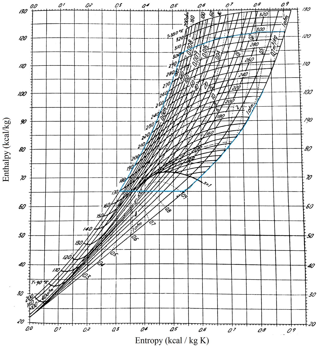
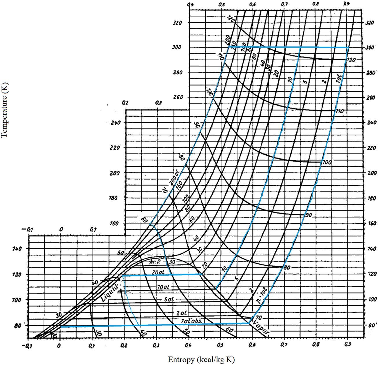
Hausen diagram: It represents temperature on the y-axis versus entropy on the x-axis (Hausen, 1926). It has parametric lines for pressure and enthalpies. Below the bell line the gas–liquid mixtures can be seen. This is the region for air liquefaction. See Fig. 3.1.

Figure 3.1 Hausen diagram. Adapted with permission from: Hausen, 1926. Hausen, H., 1926. Der Thomson-Joule-Effekt und die zustandsgrossen der Luft. C. Forsch. Arb. Ing.-Wes. Heft 274.

Mollier diagram

This diagram dates back to 1904 when Richard Mollier plotted the total heat versus entropy. There are parametric lines for pressure and temperature, and discontinuous lines for constant specific volume. See Fig. 3.2.

Figure 3.2 Mollier’s diagram. Adapted with permission from: Vancini, C.A., 1961. La sintesi dell’ammoniaca, Hoepli, Milano.

The liquefaction process

This process, devised by von Linde, consists of four basic steps. First, the gas is compressed isothermally. Next, it is cooled down at constant pressure. The gas is then expanded, and finally, the gas and liquid phases are separated.

1. Compression. This represents the only work input to the system. From basic thermodynamics it can be proved that the minimum theoretical isothermal work assuming ideal gases is given by:

$W = Δ H - T_{o} Δ S = - \int_{1}^{2} P d V = R T_{o} \ln (\frac{P_{2}}{P_{1}})$ $W = Δ H - T_{o} Δ S = - \int_{1}^{2} P d V = R T_{o} \ln (\frac{P_{2}}{P_{1}})$ (3.1)

(3.1)

2. Isobaric cooling. The noncondensed fraction of the stream is used to cool down the compressed gas.

3. Expansion. There are several alternatives to expand the gas phase. Karl von Linde in 1895 proposed the use of a valve. This expansion occurs at constant enthalpy. Later, in 1902, George Claude used an isentropic expansion, wherein a large volume contraction occurs. The work generated in this expansion can be estimated using Eqs. (3.2) and (3.3):

$W = Δ H - T_{o} Δ S = - \int_{1}^{2} p d V = P V^{k} = K$ $W = Δ H - T_{o} Δ S = - \int_{1}^{2} p d V = P V^{k} = K$ (3.2)

(3.2)

$W = \frac{n R \cdot k \cdot (T)}{((k - 1))} \frac{1}{η_{c}} ({(\frac{P_{out}}{P_{in}})}^{\frac{k - 1}{k}} - 1);$ $W = \frac{n R \cdot k \cdot (T)}{((k - 1))} \frac{1}{η_{c}} ({(\frac{P_{out}}{P_{in}})}^{\frac{k - 1}{k}} - 1);$ (3.3)

(3.3)

However, k is not constant, and thus the use of diagrams makes the computation of the work easier.

4. Phase separation. The nonliquid phase is recycled and its energy integrated to cool down the compressed air.

There are two variables that determine the efficiency of the liquefaction cycle. On the one hand, the air has to be compressed to ensure that we enter the two-phase region upon expansion (see Fig. 3.1). The work involved is the energy that the cycle consumes, and is given by Eq. (3.4):

$W = Δ H - T_{o} Δ S = R T_{o} \ln (\frac{P_{2}}{P_{1}})$ $W = Δ H - T_{o} Δ S = R T_{o} \ln (\frac{P_{2}}{P_{1}})$ (3.4)

(3.4)

On the other hand, the cooling obtained in the expansion along a constant enthalpy line could be estimated using Linde’s equation, Eq. (3.5), where k has an average value of 2·10⁴ bar⁻¹·K:

$Δ T = k \frac{P_{2} - P_{1}}{T^{2}}$ $Δ T = k \frac{P_{2} - P_{1}}{T^{2}}$ (3.5)

(3.5)

Therefore, we are interested in a high-pressure difference, $(P_{2} - P_{1}) ↑$ $(P_{2} - P_{1}) ↑$ , and low-pressure ratio, $(\frac{P_{2}}{P_{1}}) ↓$ $(\frac{P_{2}}{P_{1}}) ↓$

A simple computation for two cycles with the same pressure difference and different pressure ratio results in large energy savings (see Table 3.2). The first option consumes 3.6 times more energy.

Table 3.2

Energy Consumption in Linde’s Cycle

	Cycle 1	Cycle 2
P₁ (atm)	1	50
P₂ (atm)	150	200
P₂/P₁	150	4
P₂−P₁ (atm)	150	150
Energy (J)	360	100

Example 3.1

Check the use of Linde’s equation $(Δ T = k \frac{P_{2} - P_{1}}{T_{1}^{2}})$ $(Δ T = k \frac{P_{2} - P_{1}}{T_{1}^{2}})$ for an isenthalpic expansion with k=2·10⁴ atmK, P [=] atm and T [=] K.

Solution

Take the enthalpy line of 90 kcal/kg. For different expansions, compute the final temperature (T₂) using Linde’s equation. This value is compared to the one we read in Hausen diagram. Using the actual value for T₂, we compute the actual value for k. Table 3E1.1 shows the results. We see that the theoretical value for k=20,000 atmK is only valid in specific regions along the isenthalpic line.

Table 3E1.1

Results

	T₁ (K)	P₁ (atm)	P₂ (atm)	T₂ (eq)	T₂ (diagram)	k real
h=90 kcal/kg	233	200	150	214.5801	226	7600.46
	226	150	100	206.4213	214.5	11,747.48
	214.5	100	80	205.8063	210	10,352.31
	210	80	60	200.9297	200	22,050
	200	60	40	190	190	20,000
	190	40	30	184.4598	185.5	16,245
	185.5	30	20	179.6878	180	18,925.64
	180	20	10	173.8272	173.6	20,736
	173.6	10	5	170.2818	170	21,698.61
	170	5	2	167.9239	168.2	17,340
	168.2	2	1	167.4931	168.2	0

Linde–Hampson air liquefaction cycle

Description

The simplest alternative is a cycle comprising the four stages described earlier. Fig. 3.3 shows the flowsheet for the system. First, an isothermal compression from 1 to 2. Second, the compressed air is cooled down at constant pressure in a heat exchanger using the nonliquid fraction as cooling agent. Once the compressed air is cold enough, it is expanded through a valve, typically down to atmospheric pressure. The air is then laminated into a liquid and a gas phase. If we now describe this cycle on the Hausen diagram, we start with atmospheric air at 300K and 1 atm at point 1.

The atmospheric air is compressed from 1 atm to 200 atm at constant temperature, point 2 in Fig. 3.4 for the Hausen diagram or Fig. 3.5 for the Mollier diagram. After each compression stage, the energy generated must be removed from the system. Next, a heat exchanger is used to cool down the air from point 2 to point 3. Subsequently, the air is expanded in the valve until atmospheric pressure, point 4. We now have a gas–liquid mixture that we separate, obtaining liquid air (4′) and gas air (4″) that is the cooling agent for the heat exchanger. Therefore, we see that energy is integrated within our process. This process is also called the “simple regenerative cycle,” devised by Karl von Linde in 1895 in Munich. The actual yield to liquid air is low (Kerry, 2007).

Figure 3.4 Linde’s cycle in Hausen’s diagram.

Figure 3.5 Linde’s cycle in Mollier’s diagram.

Analysis

An energy balance is performed on the volume within the curved cornered rectangle in Fig. 3.3. Using a basis of 1 kg we have:

$1 kg H_{2} = f H_{4'} + (1 - f) H_{1'} + q$ $1 kg H_{2} = f H_{4'} + (1 - f) H_{1'} + q$ (3.6)

(3.6)

where f is the fraction of liquid air, q is the heat loss, and H_i is the enthalpy of point i. Note that in cryogenic systems the energy losses correspond to the energy that enters the system. Solving for f, we have Eq. (3.7):

$f = \frac{H_{1'} - H_{2} - q}{H_{1'} - H_{4'}}$ $f = \frac{H_{1'} - H_{2} - q}{H_{1'} - H_{4'}}$ (3.7)

(3.7)

Under ideal operating conditions, the nonliquid air exits the process under the same initial conditions that as it was fed into it.

${H'}_{1} = H_{1}$ ${H'}_{1} = H_{1}$ (3.8)

(3.8)

Furthermore, there should not be any losses (q=0). Typically this means that the heat exchanger is perfectly isolated. Therefore, the optimal fraction of liquid air obtained would be as follows:

$f = \frac{H_{1} - H_{2}}{H_{1} - {H'}_{4}}$ $f = \frac{H_{1} - H_{2}}{H_{1} - {H'}_{4}}$ (3.9)

(3.9)

Thus, the energy for compressing the air is given by Eq. (3.10):

$W = Δ H - T_{o} Δ S = (H_{2} - H_{1}) - T_{o} (S_{2} - S_{1})$ $W = Δ H - T_{o} Δ S = (H_{2} - H_{1}) - T_{o} (S_{2} - S_{1})$ (3.10)

(3.10)

where T_o is the feed temperature, which is supposed to be kept constant. Alternatively, we can compute it as (PV=constant):

$W = Δ H - T_{o} Δ S = - \int_{1}^{2} P d V = R T_{o} \ln (\frac{P_{2}}{P_{1}})$ $W = Δ H - T_{o} Δ S = - \int_{1}^{2} P d V = R T_{o} \ln (\frac{P_{2}}{P_{1}})$ (3.11)

(3.11)

Note that there are a number of simplications:

• No pressure drops are considered in the analysis.

• When the air enters the two-phase region, an equilibrium is obtained and the liquid phase gets more concentrated in the less volatile species while the gas phase is enriched with the nitrogen; thus the exit streams do not have the same composition.

• The compression should be carried out in a multicompression system where at each stage the air is heated up and later cooled down. Thus, the path from 1 to 2 is not given by a straight line, but has peaks. Typically, the compression ratio is 4–5 per stage, which avoids surpassing 204°C.

Let us illustrate the performance of the cycle with an example.

Example 3.2

Compute the liquid fraction obtained in a Linde cycle considering:

• point 1 in Fig. 3.4 is at 27°C and 1 atm, and

• point 2 is at 27°C and 200 atm.

The air is expanded to atmospheric pressure.

Solution

Molliere’s diagram and Hausen’s diagram are used in the solution of this example.

Using Molliere’s diagram:

Look for the enthalpies and entropies of the different points of the cycle in Fig. 3E2.1, corners in the cycle.

H₁=122 kcal/kg	S₁=0.9 kcal/kgK
H₂=114 kcal/kg	S₂=0.525 kcal/kgK
H_4′=22 kcal/kg	S_4′=0.0 kcal/kgK

Figure 3E2.1 Reading of the air properties for example 3.2.

Thus, assuming ideal operation of the cycle, the liquid fraction becomes:

$f = \frac{H_{1} - H_{2}}{H_{1} - H_{4'}} = \frac{122 - 114}{122 - 22} = 0.08 \frac{{kg}_{liquidair}}{{kg}_{air}}$ $f = \frac{H_{1} - H_{2}}{H_{1} - H_{4'}} = \frac{122 - 114}{122 - 22} = 0.08 \frac{{kg}_{liquidair}}{{kg}_{air}}$

Next, compute the work using either the readings from the diagram:

$W_{1 \to 2} = (H_{2} - H_{1}) - T_{o} (S_{2} - S_{1}) = (114 - 122) \frac{kcal}{kg} - 300 K (0.525 - 0.9) \frac{kcal}{kg K} = 105 \frac{kcal}{kg}$ $W_{1 \to 2} = (H_{2} - H_{1}) - T_{o} (S_{2} - S_{1}) = (114 - 122) \frac{kcal}{kg} - 300 K (0.525 - 0.9) \frac{kcal}{kg K} = 105 \frac{kcal}{kg}$

Or the equations derived from the thermodynamic model:

$W_{1 \to 2} = n R T \ln (\frac{P_{2}}{P_{1}}) = \frac{1}{29} \cdot 8.314 \cdot 300 \cdot \ln (200) = 456 kJ / kg \equiv 109 kcal / kg$ $W_{1 \to 2} = n R T \ln (\frac{P_{2}}{P_{1}}) = \frac{1}{29} \cdot 8.314 \cdot 300 \cdot \ln (200) = 456 kJ / kg \equiv 109 kcal / kg$

We see that both values are similar, within the approximation error due to our reading of the information on the diagram and the assumption of ideal gas used in Eq. (3.11). The energy computed previously is referred to one kilogram of initial air. If we refer the energy to the actual liquid produced we have:

$W_{1 \to 2} = \frac{105 \frac{kcal}{kg}}{0.08 \frac{{kg}_{liquid}}{{kg}_{air}}} = 1325 \frac{kcal}{{kg}_{liquid}}$ $W_{1 \to 2} = \frac{105 \frac{kcal}{kg}}{0.08 \frac{{kg}_{liquid}}{{kg}_{air}}} = 1325 \frac{kcal}{{kg}_{liquid}}$

The minimum in energy consumed is computed as that needed to liquefy all the initial air, assuming constant temperature, since the energy provided to the system is an isothermal compression. The standard value is T_o=300K. Thus:

$\begin{matrix} W_{\min} & = W_{1 \to 4'} = (H_{4'} - H_{1}) - T_{o} (S_{4'} - S_{1}) \\ = (22 - 122) \frac{kcal}{kg} - 300 K (0.0 - 0.9) \frac{kcal}{kg K} = 170 \frac{kcal}{kg} \end{matrix}$ $\begin{matrix} W_{\min} & = W_{1 \to 4'} = (H_{4'} - H_{1}) - T_{o} (S_{4'} - S_{1}) \\ = (22 - 122) \frac{kcal}{kg} - 300 K (0.0 - 0.9) \frac{kcal}{kg K} = 170 \frac{kcal}{kg} \end{matrix}$

Therefore, the efficiency of the cycle is computed as the ratio between the minimum work, and the work used per kg of liquid air obtained:

$η = \frac{W_{\min}}{W_{1 \to 2}} = 0.13 \approx 13 %$ $η = \frac{W_{\min}}{W_{1 \to 2}} = 0.13 \approx 13 %$

Using Hausen’s diagram:

In this case, the level rule is used to determine the temperatures before and after the expansion, T₃ and T₄. Thus, calling F the feed, L the liquefied air, and V the nonliquefied fraction, LF is the distance from point 4’ to 4 and FV, that from 4 to 4”.

$f \cdot L F = (1 - f) \cdot F V$ $f \cdot L F = (1 - f) \cdot F V$

We measure on the diagram (Fig. 3E2.2) the distance between both edges of the two-phase region, where LV=6.5 cm. Thus, we solve for LF:

$L F = \frac{1 - f}{f} F V = \frac{1 - f}{f} (6.5 - L F) \Rightarrow L F = \frac{\frac{1 - f}{f} 6.5}{1 + \frac{1 - f}{f}} = 5.98$ $L F = \frac{1 - f}{f} F V = \frac{1 - f}{f} (6.5 - L F) \Rightarrow L F = \frac{\frac{1 - f}{f} 6.5}{1 + \frac{1 - f}{f}} = 5.98$

Figure 3E2.2 Lever rule in Hausen’s diagram.

Using the distance computed, we allocate point 4 in Fig. 3E2.2. Since the expansion is isenthalpic, H₃=H₄, equal to 66 kcal/kg. Alternatively, we can compute the enthalpy by performing an energy balance to the phase separator once the liquefied fraction is known:

$1 kg \cdot H_{4} = f \cdot H_{4'} + (1 - f) H_{4 ″} = 0.08 \cdot 22 + (1 - 0.08) H_{4 ″}$ $1 kg \cdot H_{4} = f \cdot H_{4'} + (1 - f) H_{4 ″} = 0.08 \cdot 22 + (1 - 0.08) H_{4 ″}$

where H_4″ and H_4′ are equal to 70 kcal/kg and 22 kcal/kg, respectively. Thus:

$H_{4} = 66 kcal / kg$ $H_{4} = 66 kcal / kg$

Just to close the loop we can perform an energy balance to the heat exchanger to validate the heat integration.

$\begin{array}{l} 1 kg \cdot (H_{2} - H_{3}) = (1 - f) (H_{1'} - H_{4'}) \\ 1 kg \cdot (114 - 66) = (1 - f) (122 - 70) \\ 48 \approx 47.84 \end{array}$ $\begin{array}{l} 1 kg \cdot (H_{2} - H_{3}) = (1 - f) (H_{1'} - H_{4'}) \\ 1 kg \cdot (114 - 66) = (1 - f) (122 - 70) \\ 48 \approx 47.84 \end{array}$

Example 3.3

Linde’s cycle with energy losses. Compute the liquefied fraction of a system that corresponds to a modified version of example 3.2. In this case the energy loss in the system is 2 kcal/kg and the temperature difference (T₁ – T_1′) is equal to 3°C.

Solution

According to any of the diagrams, H_1′=121.3 kcal/kg (24°C and 1 atm). Performing an energy balance to the system:

$f = \frac{H_{1'} - H_{2} - q}{H_{1'} - H_{4'}} = \frac{121.3 - 114 - 2}{121.3 - 22} = 0.053 \frac{{kg}_{liquid air}}{{kg}_{air}}$ $f = \frac{H_{1'} - H_{2} - q}{H_{1'} - H_{4'}} = \frac{121.3 - 114 - 2}{121.3 - 22} = 0.053 \frac{{kg}_{liquid air}}{{kg}_{air}}$

As expected, the liquefied fraction is lower than in the ideal case. Thus, the energy to liquefy a kg of air in this case becomes:

$W_{1 \to 2} = \frac{105 \frac{kcal}{kg}}{0.053 \frac{{kg}_{liquid}}{{kg}_{air}}} = 1981 \frac{kcal}{{kg}_{liquid}}$ $W_{1 \to 2} = \frac{105 \frac{kcal}{kg}}{0.053 \frac{{kg}_{liquid}}{{kg}_{air}}} = 1981 \frac{kcal}{{kg}_{liquid}}$

And the efficiency is given by:

$η = \frac{W_{\min}}{W_{1 \to 2}} = \frac{170}{1981} = 0.0858$ $η = \frac{W_{\min}}{W_{1 \to 2}} = \frac{170}{1981} = 0.0858$

The evolution of the liquefaction processes aims to increase the liquefied fraction, improving the energy efficiency of the processes and reducing the cost of investment. From the original Linde’s cycle, there are several modifications. The first one considers the use of external cooling using ammonia. The cycle was renamed as the Linde–Hampson cycle with precooling. It is based on the fact that around −33°C the isenthalpic lines have a steeper slope. In Fig. 3.6 the flowsheet for the process and the scheme of the thermodynamic cycle are presented. Ammonia is used to cool down the compressed air. Therefore, there are three cooling steps. The first one cools the compressed air from room temperature just a few degrees. Next, ammonia is used to save cooling capacity from the nonliquefied fraction so that it is possible to cool the compressed air a bit further. The third cooling step uses the nonliquefied fraction for the final cooling of the compressed air to reach point 3 in the diagram. By doing this, the energy extracted from the system in the evaporation of the ammonia is somehow saved so that cold nonliquified air is still available to further reduce the temperature of the compressed air.

Figure 3.6 Linde–Hampson cycle with precooling.

The example here does not use either of the diagrams presented above, but uses a process simulator, CHEMCAD, to compute the liquefied fraction.

Example 3.4

Compute the liquefied fraction of a Linde–Hampson cycle with precooling using ammonia.

Solution

It is not the aim of the book to introduce the reader to the use of software for chemical engineering purposes; better textbooks can be found for that purpose (Martín, 2014). Here we only present the stages needed to build the flowsheet:

1. Format Engineering Units.

2. Select components: For CHEMCAD, air is considered as a component in itself; we also select ammonia.

3. Thermodynamics: Select the thermodynamic model to compute the mass and energy balances. In this case equations of state are recommended by the simulator.

4. Drawing the flowsheet. Use the palette to the right to drag your units from there to the main window. Bear in mind that the feeds and the products are the arrows in the palette. The compression cannot be performed in a single step since the pressure ration is large. We follow the rule of thumb:

$\sqrt[n]{\frac{P_{2}}{P_{1}}} \leq 4$ $\sqrt[n]{\frac{P_{2}}{P_{1}}} \leq 4$

Thus, we use a four-stage compression system with intercooling. The efficiency of the compressors is assumed to be 90%, and they operate as polytropic ones. After each compression stage, the air is cooled down again to the initial temperature, 300K.

The most challenging part for the simulation is the recycling of the nonliquefied air. Since the energy balance must hold, we need to have cold available in the nonliquified fraction to cool down the compressed air. We use three heat exchangers that will allow two feeds and two products each. The compressed air is the main stream, and as cooling agents we have ammonia and the nonliquefied fraction. The intermediate heat exchanger is the one using ammonia. Finally, we use a valve to reduce the pressure up to 1 atm, and a flash to separate the liquid air from the nonliquefied fraction. Fig. 3E4.1 shows the flowsheet for the example.

Figure 3E4.1 Linde–Hampson with precooling cycle simulation.

Just for reference, Fig. 3E4.2A–C shows some of the characteristics of the units involved: a compressor, a heat exchanger, and the flash unit.

Figure 3E4.2 (A) Compressor unit. (B) Initial heat exchanger. (C) Flash.

The following table shows the results of the problem. We see that we can liquefy up to 16% of the air, which is twice as much as the best value presented so far in the text (Table 3E4.1).

Table 3E4.1

Results From the Linde’s Cycle With Precooling Simulation

Stream No.	7	16	17	6
Name
- - Overall - -
Molar flow kmol/h	0.0057	0.0023	0.0023	0.0288
Mass flow kg/h	0.1651	0.0400	0.0400	0.8349
Temp C	−194.6961	−33.4446	−33.4435	−194.6961
Pres atm	200.0000	1.0000	1.0000	1.0000
Vapor mole fraction	1.000	0.0000	0.7763	1.000
Enth MJ/h	0.0000	−0.16831	−0.12519	−0.18522
Tc C	−140.7000	132.5000	132.5000	−140.7000
Pc atm	37.7400	112.7848	112.7848	37.7400
Std. sp gr. wtr=1	0.862	0.619	0.619	0.862
Std. sp gr. air=1	1.000	0.588	0.588	1.000
Degree API	32.6531	97.1314	97.1314	32.6531
Average mol wt	28.9510	17.0310	17.0310	28.9510
Actual dens kg/m3	880.5709	681.4407	1.1173	4.6153
Actual vol m3/h	0.0002	0.0001	0.0358	0.1809
Std liq m3/h	0.0002	0.0001	0.0001	0.0010
Std vap 0 C m3/h	0.1278	0.0526	0.0526	0.6464

EQUIPMENT SUMMARIES
Heat Exchanger Summary
Equip. No.	3	12	13
Name
1st Stream T Out C	1.0000	−30.0000	−111.0000
Calc Ht Duty MJ/h	0.0338	0.0431	0.1379
LMTD (End points) C	24.3340	13.4630	19.5290
LMTD Corr Factor	1.0000	1.0000	1.0000
1st Stream Pout atm	200.0000	200.0000	200.0000
2nd Stream Pout atm	1.0000	1.0000	1.0000

Example 3.5

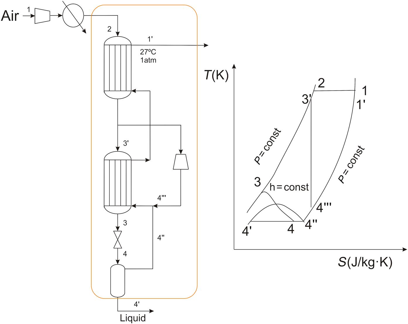
Compute the liquefied fraction obtained in the process given in Fig. 3E5.1 considering that the isenthalpic expansion occurs at 20 atm (60 kcal/kg). Determine the energy removed from the system using ammonia as the cooling agent.

Solution

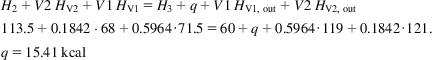
We perform a global energy balance from point 2 in Fig. 3E5.1 considering that we have two exists of nonliquid air, one at 20 atm and the other at 1 atm. Thus, following the notation on Fig. 3E5.1 and reading in Fig. 3E5.2 we have:

$H_{3} (20 atm, 160 K) = 60 kcal / kg (problem data),$ $H_{3} (20 atm, 160 K) = 60 kcal / kg (problem data),$

$H_{L1} (liq . Sat . 20 atm) = 43 kcal / kg,$ $H_{L1} (liq . Sat . 20 atm) = 43 kcal / kg,$

$H_{V 1} (vap . Sat . 20 atm) = 71.5 kcal / kg,$ $H_{V 1} (vap . Sat . 20 atm) = 71.5 kcal / kg,$

$H_{L 2} (liq . Sat . 1 atm) = 22 kcal / kg,$ $H_{L 2} (liq . Sat . 1 atm) = 22 kcal / kg,$

$H_{V 2} (vap . Sat . 1 atm) = 68 kcal / kg .$ $H_{V 2} (vap . Sat . 1 atm) = 68 kcal / kg .$

Figure 3E5.2 Thermodynamic scheme of the liquefaction process in example 3.5.

We have two expansions and thus we applied the level rule twice. For the first one,

$\begin{array}{l} F = L 1 + V 1 \\ 1 kg H_{3} = L 1 H_{L 1} + V 1 H_{V 1} \end{array}$ $\begin{array}{l} F = L 1 + V 1 \\ 1 kg H_{3} = L 1 H_{L 1} + V 1 H_{V 1} \end{array}$

where L1=0.4035 kg, V1=0.5964 kg.

For the second expansion we have the following mass and energy balances:

$\begin{array}{l} L 1 = V 2 + L 2 \\ H_{L 1} L 1 = V 2 H_{V 2} + L 2 H_{L 2} \end{array}$ $\begin{array}{l} L 1 = V 2 + L 2 \\ H_{L 1} L 1 = V 2 H_{V 2} + L 2 H_{L 2} \end{array}$

Solving the system of equations: L2=0.2192 kg, V2=0.1842 kg.

We now perform a global energy balance to compute the energy removed from the system, q:

$\begin{array}{l} 1 kg \cdot H_{2} = V 2 H_{V 2, out} + L 2 H_{L 2, out} + q + V 1 H_{V 1, out} \\ 113.5 = 0.1892 \times 121 + 0.2192 \times 22 + q + 0.5964 \times 119 \\ q = 15.42 kcal \end{array}$ $\begin{array}{l} 1 kg \cdot H_{2} = V 2 H_{V 2, out} + L 2 H_{L 2, out} + q + V 1 H_{V 1, out} \\ 113.5 = 0.1892 \times 121 + 0.2192 \times 22 + q + 0.5964 \times 119 \\ q = 15.42 kcal \end{array}$

Alternatively, we can perform the energy balance to the heat exchanger alone:

$\begin{array}{l} H_{2} + V 2 H_{V 2} + V 1 H_{V 1} = H_{3} + q + V 1 H_{V 1, out} + V 2 H_{V 2, out} \\ 113.5 + 0.1842 \cdot 68 + 0.5964 \cdot 71.5 = 60 + q + 0.5964 \cdot 119 + 0.1842 \cdot 121 \\ q = 15.41 kcal \end{array} .$ $\begin{array}{l} H_{2} + V 2 H_{V 2} + V 1 H_{V 1} = H_{3} + q + V 1 H_{V 1, out} + V 2 H_{V 2, out} \\ 113.5 + 0.1842 \cdot 68 + 0.5964 \cdot 71.5 = 60 + q + 0.5964 \cdot 119 + 0.1842 \cdot 121 \\ q = 15.41 kcal \end{array} .$

The problem can be stated differently. In case there is no precooling, compute the temperature at which we expand the stream.

Mass Balance to flash 1	F=V1+L1
Energy Balance to flash 1	F·H₃=V1 H_V1+L1 H_L1
Mass Balance to flash 2	L1=V2+L2
Energy Balance to flash 2	L1·H_L1=V2 H_V2+L2 H_L2
Global energy balance	F H₂=V2 H_{V2, out}+ L2 H_L2,out+V1 H_{V1, out}

Assuming F=1, the system consists of five equations and five variables, where

$H_{2} = 113.5 kcal / kg,$ $H_{2} = 113.5 kcal / kg,$

$H_{L 1} (liq . Sat . 20 atm) = 43 kcal / kg,$ $H_{L 1} (liq . Sat . 20 atm) = 43 kcal / kg,$

$H_{V 1} (vap . Sat . 20 atm) = 71.5 kcal / kg,$ $H_{V 1} (vap . Sat . 20 atm) = 71.5 kcal / kg,$

$H_{V 1, out} (out, 20 atm) = 123 kcal / kg,$ $H_{V 1, out} (out, 20 atm) = 123 kcal / kg,$

$H_{L 2} (liq . Sat . 1 atm) = 22 kcal / kg,$ $H_{L 2} (liq . Sat . 1 atm) = 22 kcal / kg,$

$H_{V 2} (vap . Sat . 1 atm) = 68 kcal / kg,$ $H_{V 2} (vap . Sat . 1 atm) = 68 kcal / kg,$

$H_{V 2, out} (out, 1 atm) = 121 kcal / kg .$ $H_{V 2, out} (out, 1 atm) = 121 kcal / kg .$

We solve the system using EXCEL. The results can be seen in Table 3E5.1. For further insight on the use of solver for chemical engineering problems we refer the reader to Martín (2014).

Table 3E5.1

Results

		H₂	H₃	H_sat	H_out
F	1	113.5	67.458693
L1	0.14180025			43
V1	0.85819975			71.5	121
L2	0.07706535			22
V2	0.0647349			68	123
	M balance flash 1	1	1	0
	E balance flash 1	67.458693	67.458693	0
	M balance flash 2	0.14180025	0.14180025	0
	E balance flash 2	6.0974106	6.0974106	0
	Global balance	113.5	113.5	0

Claude’s cycle

Description

There are other alternatives to increase the liquefied fraction. In 1902 George Claude from the University of Paris used an expansion engine that was reversible and adiabatic so that the expansion was isentropic. Thus in the Claude cycle the air (or another gas) is compressed, typically to 40 atm. After cooling using nonliquefied fractions, a fraction is diverted and expanded. The expanded gas is mixed with the cold nonliquefied gas so that the mixture is used to cool down the compressed air. The diverted fraction is around 75% of the feed. See Fig. 3.7 for the flowsheet and the thermodynamic cycle. This technique was welcomed in the industry at the time since it required lower operating pressures and increased energy efficiency. The isentropic efficiency is defined as the ratio between the actual enthalpy difference in the expansion and the enthalpy difference for the ideal isentropic case (Fig. 3.8).

Figure 3.7 The Claude cycle for air liquefaction.

Analysis

1 kg of fed air undergoes the following path along the flowsheet.

Performing an energy balance to the discontinuous line rectangle we have:

$1 kg H_{2} + q = f g H_{4'} + [(1 - f) g + (1 - g)] H_{1'} + W_{Δ S = 0}$ $1 kg H_{2} + q = f g H_{4'} + [(1 - f) g + (1 - g)] H_{1'} + W_{Δ S = 0}$ (3.12)

(3.12)

$W_{Δ S = 0} = (1 - g) (H_{3'} - H_{4 ‴})$ $W_{Δ S = 0} = (1 - g) (H_{3'} - H_{4 ‴})$ (3.13)

(3.13)

$1 kg H_{2} + q = f g H_{4'} + [(1 - f) g + (1 - g)] H_{1'} + (1 - g) (H_{3'} - H_{4 ‴})$ $1 kg H_{2} + q = f g H_{4'} + [(1 - f) g + (1 - g)] H_{1'} + (1 - g) (H_{3'} - H_{4 ‴})$ (3.14)

(3.14)

$f = \frac{(H_{2} - H_{1'}) - (1 - g) (H_{3'} - H_{4 ‴}) + q}{g (H_{4'} - H_{1'})}$ $f = \frac{(H_{2} - H_{1'}) - (1 - g) (H_{3'} - H_{4 ‴}) + q}{g (H_{4'} - H_{1'})}$ (3.15)

(3.15)

Under ideal conditions:

$q = 0, H_{1'} \to H_{1}$ $q = 0, H_{1'} \to H_{1}$ (3.16)

(3.16)

Thus:

$f = \frac{(H_{1} - H_{2}) + (1 - g) (H_{3'} - H_{4 ‴})}{g (H_{1} - H_{4'})}$ $f = \frac{(H_{1} - H_{2}) + (1 - g) (H_{3'} - H_{4 ‴})}{g (H_{1} - H_{4'})}$ (3.17)

(3.17)

To evaluate the cycle we propose the following example.

Example 3.6

Compute the liquefied fraction obtained in a Claude cycle where the air is compressed up to 40 atm, and the diverted fraction to the expansion machine is 75%. Assume that (H_3′–H_4″′) is equal to 17 kcal/kg.

Solution

In any of the above presented diagrams we read:

$\begin{array}{l} H_{1} = H_{1'} = 122 kcal / kg \\ H_{4'} = 22 kcal / kg \\ H_{2} = 119 kcal kg \end{array}$ $\begin{array}{l} H_{1} = H_{1'} = 122 kcal / kg \\ H_{4'} = 22 kcal / kg \\ H_{2} = 119 kcal kg \end{array}$

Substituting in Eq. (3.17):

$\begin{array}{l} f = \frac{(H_{1} - H_{2}) + (1 - g) (H_{3'} - H_{4 ‴})}{g (H_{1} - H_{4'})} = \frac{122 - 119 + 0.75 \cdot 17}{0.25 \cdot (122 - 22)} = 0.63 \\ f g = 0.63 \cdot 0.25 = 0.1575 \frac{{kg}_{liquid air}}{{kg}_{air}} \end{array}$ $\begin{array}{l} f = \frac{(H_{1} - H_{2}) + (1 - g) (H_{3'} - H_{4 ‴})}{g (H_{1} - H_{4'})} = \frac{122 - 119 + 0.75 \cdot 17}{0.25 \cdot (122 - 22)} = 0.63 \\ f g = 0.63 \cdot 0.25 = 0.1575 \frac{{kg}_{liquid air}}{{kg}_{air}} \end{array}$

To compute the work required it is assumed that the power obtained in the expansion is accounted for as produced for the global energy balance:

$\begin{array}{l} W_{1 \to 2} = H_{2} - H_{1} - T_{o} (S_{2} - S_{1}) = 119 - 122 - 300 (0.655 - 0.905) = 72 \frac{kcal}{kg} \\ W_{aportar} = \frac{W_{1 \to 2} - W_{3 \to 4 ‴}}{f g} = \frac{72 - 0.75 \cdot 17}{0.1575} = 376 \frac{kcal}{{kg}_{liquid air}} \\ η = \frac{W_{\min}}{W_{provided}} = \frac{170}{376} = 0.45 \end{array}$ $\begin{array}{l} W_{1 \to 2} = H_{2} - H_{1} - T_{o} (S_{2} - S_{1}) = 119 - 122 - 300 (0.655 - 0.905) = 72 \frac{kcal}{kg} \\ W_{aportar} = \frac{W_{1 \to 2} - W_{3 \to 4 ‴}}{f g} = \frac{72 - 0.75 \cdot 17}{0.1575} = 376 \frac{kcal}{{kg}_{liquid air}} \\ η = \frac{W_{\min}}{W_{provided}} = \frac{170}{376} = 0.45 \end{array}$

Comparing these results with the previous ones, we see that the yield to liquid air is similar to the one obtained for the precooled Linde cycle, but the energy required is far lower.

Phillips’s cycle

The cycle is similar to the Linde’s one, but in this case the cooling occurs at constant specific volume, which increases the efficiency. Fig. 3.9 represents the thermodynamic cycle using the Mollier diagram. For the evaluation of this cycle, it is the most appropriate diagram.

To illustrate the performance of this cycle, consider example 3.7.

Example 3.7

Air at 27°C and 15 atm is compressed up to 200 atm, removing the heat generated. The air is next cooled at constant volume until it reaches the saturation point. A valve is used to expand the air to 1 atm. Compute the efficiency of the Phillips’s cycle described.

Using Mollier’s diagram we read the enthalpies and entropies of the different points of the process.

H₁=121.6 kcal/kg	S₁=0.7236 kcal/kgK
H₂=114 kcal/kg	S₂=0.525 kcal/kgK
H_4′=22 kcal/kg	S_4′=0.0 kcal/kgK

An enthalpy balance is formulated assuming ideal behavior of the cycle.

$\begin{array}{l} 1 kg \cdot H_{2} = f \cdot H_{4'} + (1 - f) \cdot H_{1} \Rightarrow f = \frac{H_{1} - H_{2}}{H_{1} - H_{4'}} \\ f = 0.076 {kg}_{liquid} {/ kg}_{air} \end{array}$ $\begin{array}{l} 1 kg \cdot H_{2} = f \cdot H_{4'} + (1 - f) \cdot H_{1} \Rightarrow f = \frac{H_{1} - H_{2}}{H_{1} - H_{4'}} \\ f = 0.076 {kg}_{liquid} {/ kg}_{air} \end{array}$

This value is slightly larger than the one obtained with the Linde’s simple cycle method. Next, the energy requirement is computed as follows:

$W_{1 \to 2} = (H_{2} - H_{1}) - T_{o} (S_{2} - S_{1}) = (114 - 121.6) - 300 \cdot (0.525 - 0.736) = 55.4 \frac{kcal}{kg}$ $W_{1 \to 2} = (H_{2} - H_{1}) - T_{o} (S_{2} - S_{1}) = (114 - 121.6) - 300 \cdot (0.525 - 0.736) = 55.4 \frac{kcal}{kg}$

It is the smallest value seen so far when comparing the different cycles. As per kg of liquid air:

$W_{1 \to 2} = \frac{55.4 \frac{kcal}{kg}}{0.076 \frac{{kg}_{liquid air}}{{kg}_{air}}} = 729 \frac{kcal}{{kg}_{liquid air}}$ $W_{1 \to 2} = \frac{55.4 \frac{kcal}{kg}}{0.076 \frac{{kg}_{liquid air}}{{kg}_{air}}} = 729 \frac{kcal}{{kg}_{liquid air}}$

The minimum theoretical work is given as that required to obtain a kilogram of liquid air:

$\begin{matrix} W_{\min} & = W_{1 \to 4'} = (H_{4'} - H_{1}) - T_{o} (S_{4'} - S_{1}) \\ = (22 - 121.6) \frac{kcal}{kg} - 300 K (0.0 - 0.736) \frac{kcal}{kg K} = 120.9 \frac{kcal}{{kg}_{liquid air}} \end{matrix}$ $\begin{matrix} W_{\min} & = W_{1 \to 4'} = (H_{4'} - H_{1}) - T_{o} (S_{4'} - S_{1}) \\ = (22 - 121.6) \frac{kcal}{kg} - 300 K (0.0 - 0.736) \frac{kcal}{kg K} = 120.9 \frac{kcal}{{kg}_{liquid air}} \end{matrix}$

And the yield results in:

$η = \frac{W_{\min}}{W_{1 - 2}} \cdot 100 = 16.58 % > example 3.2$ $η = \frac{W_{\min}}{W_{1 - 2}} \cdot 100 = 16.58 % > example 3.2$

Cascade cycle

This method can be dated back to 1890 when Kamerlingh-Onnes in Leyden used a series of refrigerants for his experimental work on cryogenics. Further development by Keesom in 1930 provided the highest efficiency in liquefaction so far. In this scheme, each refrigerant has a boiling point in decreasing order. Typically we use ammonia, ethylene, methane, and nitrogen. Their boiling points are 240K, 189K, 112K, and 77K, respectively. See Fig. 3.10 for the flowsheet. The advantage of the cycle is that it piece-wise approximates an ideal reversible cycle, resulting in an efficient thermodynamic process. The expansion takes place through a valve at low pressure, with a low increase in entropy. In spite of its efficiency, the refrigerant losses (leaks), the complexity of the operation, and the high investment have prevented its use in air separation (Kerry, 2007). Table 3.3 shows the energy involved per kg of liquid air obtained. We need 1.7 kg of initial feed of air, and the energy is 464 kcal/kg_liquid. The liquid fraction increases up to 0.59 kg_{liquid air}/kg air (Vancini, 1961).

Table 3.3

Energy Consumption in the Cascade Cycle (Vancini, 1961)

Species	Energy Cost
1.70 kg Air	200 kcal
0.33 kg NH₃	44 kcal
0.96 kg C₂H₄	90 kcal
0.66 kg CH₄	130 kcal
	464 kcal

Air distillation

Air liquefaction is the first stage in separating air into its components. When the vapor–liquid equilibrium is established, the vapor phase gets concentrated in the volatile component and vice versa. The boiling points of nitrogen (T_b=77.3K) and oxygen (T_b=90.1K) result in them being obtained from the top and bottom of the column, respectively (Latimer, 1967). Before feeding the air into the columns it is compressed, filtered, cleaned (using molecular sieves to remove water, CO₂, and other impurities), and then cooled down to almost liquefaction (Timmerhaus and Flynn, 1989).

Linde’s Simple Column

This is the simplest process to separate air into its components. It was industrially used at the beginning of the XX century. The system consists of a single column that operates slightly above atmospheric pressure. The feed to the column is cold air from a liquefaction process. The compressed air is cooled using the separated nitrogen and oxygen (see Fig. 3.11), and it is used as hot utility. It boils the oxygen, and is then expanded before it is fed into the column. The column operates as a stripping one. As the air rises through the column it gets concentrated in nitrogen, the most volatile of the two. A stream rich in nitrogen exits from the top while another stream rich in oxygen is obtained from the bottom. The purity limit in the nitrogen is limited since no rectification section of the column is present (see Fig. 3.12). The slope of the q line depends on the fraction of liquid that we can obtain after cooling and expanding the air. The oxygen is recovered over the liquid, and has a composition of around 95% oxygen because it carries the argon, while for the top the nitrogen is recovered at 90% purity, as seen in the XY diagram.

Figure 3.12 X–Y diagram for the simple column.

Simple Column With Recycle

Recompression: The simple column design evolved to improve the purity of the nitrogen. To achieve that, part of the nitrogen from the top of the column is recompressed, cooled by using it as hot utility in the boiler of the column, expanded, and fed as if it were the reflux of the column. The compressed air is also used as hot utility in the reboiler. See Fig. 3.13A for the scheme of the system.

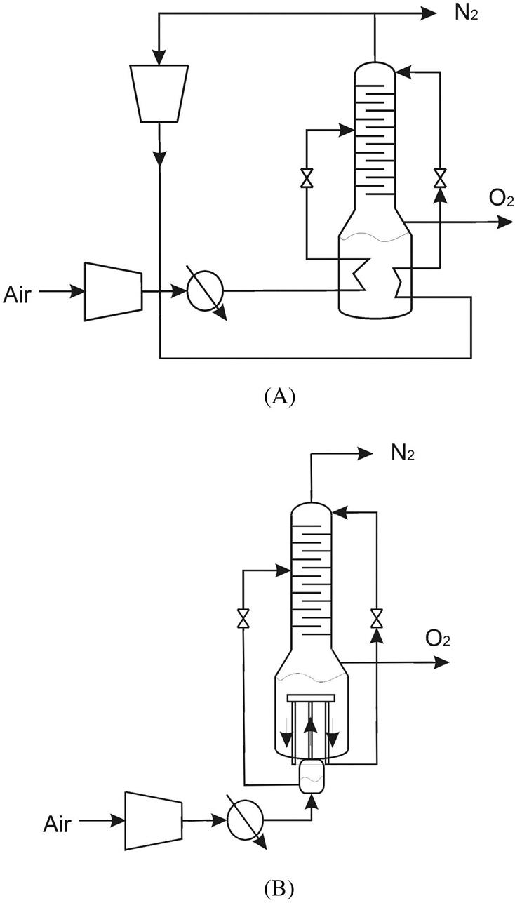
Claude’s Column: Claude also presented his design for a distillation column. It had a dephlegmator kind of device so that the compressed air at 25 atm was fed to the column. In a tubular device submerged in liquid air, the compressed gas rises. Part of the vapor liquefies and returns to the feed chamber. The gas phase, rich in nitrogen, goes down via two lateral pipes, and also liquefies. The nitrogen is gathered at the annular space and is used as recycle for the column. The liquid oxygen is fed to the column after expansion. See Fig. 3.13B for a scheme of the device.

Linde’s Double Column

Linde’s double column represented a technological breakthrough. The system consists of two columns that operate at different pressures (see Fig. 3.14). The low-pressure column typically works at 1 atm, and the higher-pressure column works at 5 atm. Air is used as hot utility in the high-pressure column so that it cools down. Next, it is expanded to obtain a liquid fraction and fed to the column. The bottoms of the column, recovered over the liquid of the high-pressure column reboiler, are expanded to 1 atm and fed to the lower-pressure column. The distillate of the high-pressure column is also expanded to 1 atm and used as reflux. This stream, rich in nitrogen, is fed at the top of the lower-pressure column. Therefore, only two streams are obtained from the system, both from the low-pressure column. From the bottoms, at about 90K, a stream rich in oxygen exits the system. The concentration is no more that 95%, due to the presence of argon in this stream. From the top, a stream rich in nitrogen at about 78K is produced.

Both columns are thermally coupled (see Fig. 3.14). The condenser of the high-pressure column acts as a reboiler for the higher-pressure column. For heat to be exchanged, a temperature gradient must be maintained. In this configuration, a temperature difference of about 4–5K is typically used. This temperature difference can be proven using the equilibrium diagrams. Typically there is no stripping region in the higher-pressure column since the operation of the upper column increases the oxygen concentration of the bottoms efficiently. The bottoms of the high-pressure column contain around 40% oxygen.

Example 3.8

Evaluate the operation of Linde’s double column. The low- and high-pressure columns work at 1 atm and 5 atm, respectively. The products are N₂, 98% molar, and O₂, with a purity of 96%. The air fed to the system is at 120K and 200 atm.

Solution

Antoine vapor pressure equation for N₂: $\ln (P_{v}) = (14.9542 - \frac{588.72}{(T (° C) + 273.15 - 6.6)})$ $\ln (P_{v}) = (14.9542 - \frac{588.72}{(T (° C) + 273.15 - 6.6)})$

Antoine vapor pressure equation for O₂: $\ln (P_{v}) = (15.4075 - \frac{734.55}{(T (° C) + 273.15 - 6.45)})$ $\ln (P_{v}) = (15.4075 - \frac{734.55}{(T (° C) + 273.15 - 6.45)})$

We assume ideal behavior for both cases and compute the XY diagram for the system as follows:

$\begin{array}{l} y_{N_{2}} = \frac{P_{Vap, N_{2}} x}{P_{Total}} \\ P_{T} = P_{O_{2}} + P_{N_{2}} = y_{O_{2}} \cdot P_{Total} + y_{N_{2}} \cdot P_{Total} = P_{Vap, O_{2}} (1 - x) + P_{Vap, N_{2}} x \to x = \frac{P_{Total} - P_{Vap, O_{2}}}{P_{Vap, N_{2}} - P_{Vap, O_{2}}} \end{array}$ $\begin{array}{l} y_{N_{2}} = \frac{P_{Vap, N_{2}} x}{P_{Total}} \\ P_{T} = P_{O_{2}} + P_{N_{2}} = y_{O_{2}} \cdot P_{Total} + y_{N_{2}} \cdot P_{Total} = P_{Vap, O_{2}} (1 - x) + P_{Vap, N_{2}} x \to x = \frac{P_{Total} - P_{Vap, O_{2}}}{P_{Vap, N_{2}} - P_{Vap, O_{2}}} \end{array}$

The operating line for the rectifying section is obtained by performing a mass balance to the higher section of the column:

$V_{n} = L_{n - 1} + D (Low pressure)$ $V_{n} = L_{n - 1} + D (Low pressure)$

$V_{n} y_{n} = L_{n - 1} x_{n - 1} + D \cdot x_{D} \to y_{n} = \frac{L_{n - 1}}{V_{n}} x_{n . - 1} + \frac{D}{V_{n}} x_{D}$ $V_{n} y_{n} = L_{n - 1} x_{n - 1} + D \cdot x_{D} \to y_{n} = \frac{L_{n - 1}}{V_{n}} x_{n . - 1} + \frac{D}{V_{n}} x_{D}$

$V_{n} + D_{2} = L_{n - 1} + D_{1} (High pressure)$ $V_{n} + D_{2} = L_{n - 1} + D_{1} (High pressure)$

$V_{n} y_{n} + D_{2} x_{D, 2} = L_{n - 1} x_{n - 1} + D \cdot x_{D, 1} \to y_{n} = \frac{L_{n - 1}}{V_{n}} x_{n . - 1} + \frac{D_{1} x_{D, 1} - D_{2} x_{D, 2}}{V_{n}}$ $V_{n} y_{n} + D_{2} x_{D, 2} = L_{n - 1} x_{n - 1} + D \cdot x_{D, 1} \to y_{n} = \frac{L_{n - 1}}{V_{n}} x_{n . - 1} + \frac{D_{1} x_{D, 1} - D_{2} x_{D, 2}}{V_{n}}$

The corresponding operating line for the stripping section is as follows:

$V_{m} = L_{m - 1} - W$ $V_{m} = L_{m - 1} - W$

$V_{m} y_{m} = L_{m - 1} x_{m - 1} + W x_{w} \to y_{m} = \frac{L_{m - 1}}{V_{m}} x_{m - 1} + \frac{W}{V_{m}} x_{W}$ $V_{m} y_{m} = L_{m - 1} x_{m - 1} + W x_{w} \to y_{m} = \frac{L_{m - 1}}{V_{m}} x_{m - 1} + \frac{W}{V_{m}} x_{W}$

..................Content has been hidden....................

You can't read the all page of ebook, please click here login for view all page.

Table of Contents for Chapter 3. Air

Create new playlist

Sign In

Sign Up

Air

Abstract

Keywords

3.1 Introduction

3.1.1 Composition

3.1.2 Uses

3.2 Air Separation

3.2.1 History

3.2.2 Classification of Air Separation Methods

A Physical separation

B Chemical separation

3.2.2.1 Physical separation

3.2.2.1.1 Cryogenic methods: air liquefaction and distillation

Mollier diagram

The liquefaction process

Linde–Hampson air liquefaction cycle

Claude’s cycle

Phillips’s cycle

Cascade cycle

Air distillation

Table of Contents for
Chapter 3. Air