
We assume that the flows of the species are approximately constant across each section of the column:
The feed to the column is partially liquid. Thus we define the liquid and vapor fraction of the feed as ![]() and
and ![]() , respectively:
, respectively:
Thus the q line can be written as follows:
We now present the mass balances. See Fig. 3E8.1 for the flow across the low-pressure column.

Low-pressure column:
Let f be the liquefied fraction from stream D2 and g the liquefied fraction from stream R2:

Thus the operating lines at the rectifying and stripping sections, as well as the q line, are given as follows:
f corresponds to a flowrate of pure saturated nitrogen at 5 atm and −178°C that is expanded to 1 atm. In the Hauser diagram we can see the result of that expansion (see Fig. 3E8.2). Using the lever rule we can compute the liquefied fractions. We assume that both streams are air, and thus the Hauser diagram can be used to compute both:

Solving the mass balances (see Table 3E8.1), we compute the operating lines. Next, we use the McCabe method to determine the number of trays needed in the low-pressure column (see Fig. 3E8.3).
Table 3E8.1
Results of Low-Pressure Column
| F | D | R | ||||
| Feed | 100 | 80.4347836 | 19.652174 | −1E-06 | ||
| Feed N2 | 79 | 78.0217401 | 0.97826087 | 79.000001 | ||
| y | L/V | D/V | L1 | 34.9999959 | ||
| Rectifying | 0.4882486 | 0.49639886 | L1′ | 80.244566 | ||
| y | L′/V′ | R/V′ | V1 | 71.6847847 | ||
| Stripping | 1.32243618 | 0.01612181 | V1′ | 60.6793487 |


High-pressure column:
The energy balances to the condenser–reboiler couple both columns and determine the flows at the high-pressure column (Fig. 3E8.4):

A mass balance to the feed tray is as follows:
where h is the liquefied fraction in the feed to the column. Thus the operating lines and the q line are as follows:
In Table 3E8.2 we present the results of the mass balances and the operating lines. Next, using the McCabe method, the number of trays needed at the high-pressure column is six (Fig. 3E8.5).


Argon separation and purification
Argon is a valuable product that is in relatively high quantities in the air. It is possible to modify the double column to obtain argon from air (see Fig. 3.15). A stream from the low-pressure column is extracted at the level where Ar concentration is maximum, around 12%. This vapor is rectified in an auxiliary column that uses a partial condenser. As refrigerant of the second column, a fraction of the oxygen stream from the bottoms of the high-pressure column is used, after expansion. The bottoms of the auxiliary column are returned to the low-pressure column, while the distillate is the Ar produced at 98% purity. Oxygen is the main impurity of the Ar and can be eliminated using chemical separation, for instance, deoxoreactors where water is produced from the oxygen impurity.

Neon can also be separated. It is more volatile than nitrogen and can be obtained by rectification of the liquid product from the top of the high-pressure column. Neon comes with nitrogen and helium as impurities.
The evolution of liquefaction and separation processes has resulted in the current liquefaction processes (Linde, 2015). Fig. 3.16 shows the flowsheet of the typical layout of one of those plants. In the first stage air is compressed. Next, it is purified using molecular sieves to remove moisture, dust, and other impurities such as CO2 or hydrocarbons. Then, the compressed air is cooled down using nonliquid oxygen and nitrogen. Subsequently, a double distillation column (Linde’s design) with an auxiliary column for Ar recovery is used. The products obtained are not only gaseous oxygen and nitrogen, but also liquid oxygen and nitrogen. The oxygen comes from the bottoms of the low-pressure column, and the nitrogen from the top of the low-pressure column.

Storage
Two storage devices can be highlighted: vacuum insulated tanks and dewars. Vacuum insulated tanks consist of a double-walled vessel. The internal wall is made of stainless steel and the outer wall is made of carbon steel. Between them the chamber is under vacuum, filled with perlite as insulation. The size of these tanks range from 1 m3 on, and they are typically designed for 14 atmg. It is also possible to have an evaporator to control the pressure inside the tank and another one to serve gas products. Dewars are cryogenic mobile devices. They also have the same double-wall structure as the tanks. Their size ranges from liters to 1 m3, and the designed pressure is 1.4 atmg. The discharge is carried out from the bottoms, and they have an internal evaporator for pressure control. Fig. 3.17 shows schemes for both.

3.2.2.1.2 Noncryogenic air separation
From an industrial perspective, liquid gases are expensive, but sometimes they are regasified for further use. Thus, a number of technologies have been developed to separate the air components without need for liquefaction. In this section, we discuss two alternatives, the use of pressure or temperature cycles known as Pressure Swing Adsorption (PSA) and Temperature Swing Adsorption (TSA), and the use of membranes. Note that these technologies are not fully developed, but they are gaining attention in the market.
Pressure Swing Adsorption cycles
The use of PSA cycles to produce oxygen or nitrogen is based on the adsorption of one of the two on a bed of particular material. Typically, since air is free, in industry there is no recovery of the purge or the adsorbed species. The operation of these cycles consists of four stages: (a) pressurization, (b) adsorption, (c) depressurization, and (d) desorption. In order to ensure continuous operation of the plant, two beds operate in parallel at any one time. Fig. 3.18 shows the operation of the cycle and the pressure at the bed. An excess in the purge increases the purity of the effluent. A defect results in higher contamination.

Unlike TSA, PSA systems do not degrade the adsorbent and can operate longer without substitution. However, the presence of moisture and drops must be avoided. Filters are used to remove them before the air is fed to the PSA system.
The production of nitrogen above 99.5% purity consists of adsorbing the oxygen out of the air. The bed for this process consists of molecular sieves, either Zeolite 4 A or active carbon Bergbau–Foschung operating at 6–8 atmg. Desorption occurs at atmospheric pressure. The purge stream consists of oxygen at 35–50% by volume. The energy consumption in the production of nitrogen is around 0.1 kWh/Nm3, and presents a lower investment than required for cryogenic units.
The production of oxygen uses a PSA system where the adsorbent is either Zeolite 13X or 5 A to adsorb the nitrogen. The working conditions are 1–3 atmg for adsorption, but the oxygen production cannot surpass 1500 Nm3/h. Furthermore, the oxygen produced has a low purity, lower than 90%, and contains Ar and N.
Apart from PSA systems for the production of oxygen, Vacuum Pressure Swing Adsorption can be used. In this case, gas desorption occurs below atmospheric pressure, 0.5 atmg. These units can produce up to 50 t/d, with more or less the same purity as the PSA systems (Pressure Swing Adsorption Picks Up Steam, 1988).
Membranes
Gas separation using membranes is based on the different diffusion rates of the species. It is a process governed by Henry’s and Fick’s Laws. The permeability, a measure of the capacity of the membrane to transport gases, is the product between the Henry’s Law constant and the diffusivity coefficient. The permeate is concentrated in the quicker-diffusing gases while the reject or purge comprises the slower-diffusing gases (Membranes, 1990).
Fick’s Law dictates the diffusion rate:
(3.18)
where Di is the diffusivity (m2/s) of species i across the membrane, ci is the concentration across the membrane, and z the distance. At steady state, we can compute the flux of component i across the membrane as follows:
(3.19)
where δ is the thickness of the membrane. Thus, assuming that two gas phases are in contact through a membrane, to the left we have a total pressure P1 and a partial pressure of each component given by:
(3.20)
To the right, we have P2. For component i to diffuse, P1>P2. Fig. 3.19 shows the scheme of the process. Gas solubility in polymers, the membrane, is assumed to follow Henry’s Law (Perry and Green, 1997).
Henry’s Law states:
(3.21)
Thus
(3.22)
where permeability is computed as ![]() . The relative permeability of one gas compared to another depends on the molecule size and the interactions with the polymeric membrane. We can establish a relative scale of diffusion rate of the main gases involved in chemical processes:
. The relative permeability of one gas compared to another depends on the molecule size and the interactions with the polymeric membrane. We can establish a relative scale of diffusion rate of the main gases involved in chemical processes:
Nitrogen and oxygen diffuse slowly across membranes while CO2 is five times quicker than oxygen. Water vapor can go through polar membranes easily, but not as easily across nonpolar polymers. This relative diffusion velocity results in the composition of the resulting permeate and reject phases. Based on the velocity, membranes are typically used to obtain nitrogen at 93–99%.
(3.23)
The separation factor provided by a membrane, Si,j, is defined as the ratio in concentrations of two species at both sides of the membrane:
(3.24)
 (3.24)
The selectivity of the membrane to both gases, ![]() , is the limit of the separation fraction for a certain pressure difference.
, is the limit of the separation fraction for a certain pressure difference.
3.2.2.2 Chemical separation
These systems are based on the reactivity of the different gases in the mixture. Oxygen is much more reactive, generating some oxide and liberating the nitrogen. The deoxo process can be used to remove the traces of oxygen as water using hydrogen as reactant. Alternatively, we can have processes like 2BaO+O2↔2BaO2 that go forward at 500°C and backward to recover the oxygen at 700°C.
Selection of the methods depends on two factors: production capacity and purity of the gas required. Membranes are typically used for 1–1000 Nm3/h of nitrogen and purities up to 99%. PSA can be used when slightly higher purity is needed, up to 10,000 Nm3/h. Higher purity and production capacity requires the use of cryogenic fractionation. In the case of oxygen production, PSA is recommended for 1–1000 Nm3/h and up to 95% purity. Any other purity requires cryogenic fractionation.
Table 3.4 shows a brief comparison of the technologies discussed. It presents the status of the maturity of the technology, the relative economics, the purity of the products, and operating limitations (Smith and Klosek, 2001).
Table 3.4
Comparison of Air Separation Technologies
| Process | Status | Economics | Byproduct Capability | Purity Limit (% volume) | Startup/Shutdown Time |
| PSA | Semimature | $$$$$$ | Poor | 95 | Minutes |
| Chemical | Developing | Unknown | Poor | >99 | Hours |
| Cryogenic | Mature | $$ | Excellent | >99 | Hours |
| Membrane | Semimature | $ | Poor | 40 | Hours |

3.3 Atmospheric pollution
There are two main sources of atmospheric pollution: natural, due to processes such as fire, volcanoes, fogs, etc., and artificial, due to human activities. Among them we can find phenomena like city smog, industrial smog, and the presence of gaseous species such as NOx, SO2, CO, CO2, smoke, or odors.
3.4 Humid air
Air can have a certain amount of moisture as a function of the conditions. Assuming ideal behavior, the total pressure results from the contribution of both gases, the air and the vapor:
(3.25)
Vapor pressure is a function of the temperature. Thus the higher the temperature the larger the amount of water vapor that the air can hold. If the air cannot handle a certain amount of water, then it condenses. This occurs for vapor pressures above the saturation at a certain temperature. Bear in mind that the presence of water vapor in air is an industrial problem for several processes. For instance, when dealing with solids, humidity can cause agglomeration, reducing the quality of the product (eg, detergents). In other cases, such as in the production of sulfuric acid, the presence of vapor generates the acid over time, representing a safety problem due to the corrosion of the pipes and reactor.
Here, the concepts of humid air are presented before they are applied to some simple examples.
(3.28)
We can use Antoine correlations to compute the saturation vapor pressure. In the case of water, we can use the following equations:
(3.29)
 (3.29)
Similarly, we can proceed for other vapor species such as ethanol or ammonia.
Example 3.9
Evaluate the process that transforms stream 1 from its initial conditions to the final ones given below. Determine whether water condenses, and compute the heat load for cooling this stream.
Stream 1, initial conditions: P=750 mmHg, T=40°C, φ=0.7
Stream 1, final conditions: P=2550 mmHg, T=22°C
Solution
If the specific moisture at the beginning is larger than that at the end, water must condense since the air cannot hold the difference. Thus, using the concepts presented above, both specific moisture contents at the beginning and at the end, assuming saturation, are as follows:
Since yfinal<yini, water must condense. For 100 kg of dry air, initially 103.37 kg of gas are compressed (100·(1+yini)) and cooled. The gas phase at the end of the process consists of 100.48 kg, (100·(1+yfinal)); therefore the difference, 2.89 kg, has to condense. We now perform an energy balance:

Example 3.10
Determine if mixing of the following two streams results in water condensation. The working pressure is 760 mmHg.
| Stream 1 | 100 kgda/s, T=54°C, φ=0.95 |
| Stream 2 | 100 kgda/s, T=9.6°C, φ=0 |
Solution
Stream 1

Stream 2
Similarly:
Mass balance to water (assuming no condensation):

For energy balance, we compute the temperature of the mixture:
At this temperature, with the computed specific moisture, the relative humidity becomes:
φ=1.46>1→Water condenses
Therefore the mass and energy balances must consider the condensed water, COND:
Energy balance:

Mass balance to water:
This is a complex problem to solve. We present here two methods: EXCEL and GAMS. For further details on the use of these packages, the reader can find the basics in Martín (2014).
EXCEL
We define the variables in different cells and use “solver” as shown in Fig. 3E10.1.
| m1 | 100 |
| m2 | 100 |
| H1 | 76.1 |
| H2 | 2.3 |
| y1 | 0.1045 |
| y2 | 0 |
| Tm (G14) | 39.7656916 |
| Pv | 54.5073231 |
| Hm | 39.0271005 |
| Ym | 0.04790204 |
| COND (G18) | 0.86959147 |
| Balance(G19) | 2.1368E-09 |

GAMS
In this case we define the data as scalar, the variables to be computed as positive variables, and write the equations of the problem by hand:
Scalar
mass1 /100/
mass2 /100/
T1 /54/
T2 /9.6/
phi1 /0.95/
phi2 /0/
Ptotal /760/;
positive variables
y1, y2, H1, H2, Hm, COND, ysat, Pv1, Pv2, Pvm, Tm;
variable
Z;
equations
BM, BE, y_1, y_2, H_1, H_2, pv_1, pv_2, H_sat, y_sat, pv_sat, obj;
BM.. mass1*y1+mass2*y2 =E= (mass1+mass2)*ysat +COND;
BE.. mass1*H1+mass2*H2=E=(mass1+mass2)*Hm+ COND*Tm;
H_1.. H1 =E= (0.24+0.46*y1)*T1+597.2*y1;
y_1.. y1 *(Ptotal-phi1*Pv1)=E= 0.62*phi1*Pv1;
pv_1.. Pv1 =E= exp(18.3036-3816.44/(227.02+T1));
H_2.. H2 =E= (0.24+0.46*y2)*T2+597.2*y2;
y_2.. y2 *(Ptotal-phi2*Pv2)=E= 0.62*phi2*Pv2;
pv_2.. Pv2 =E= exp(18.3036-3816.44/(227.02+T2));
H_sat.. Hm =E= (0.24+0.46*ysat)*Tm+597.2*ysat;
y_sat.. ysat *(Ptotal-Pvm)=E= 0.62*Pvm;
pv_sat.. Pvm =E= exp(18.3036-3816.44/(227.02+Tm));
Tm.LO=0;
Tm.UP=100;
obj.. Z =E= 2;
Model Ejem10 /all/;
solve Ejem10 Using NLP Maximizing Z
Example 3.11
Compute the temperature that a stream of air at 800 mmHg, that at 20°C has a relative moisture of 0.85, has to be heated to so that when mixed with a second stream of air, whose dew point is 50°C, does not cause water to condense.
Solution
We draw the psychometric diagram for 800 mmHg. To do that, for each temperature, compute the vapor pressure using the Antoine equation, and with it, the specific humidity at saturation using Eq. (3.26). See Fig. 3E11.1.

Next, the specific moisture of the second stream is computed. Since it is saturated at 50°C, y2 is equal to 0.08. We draw a horizontal line at y equal to 0.08. Subsequently, we allocate the initial point representing steam 1. At 20°C, φ is equal to 0.85. Thus y1 is equal to 0.012. See the square in Fig. 3E11.1.
In order for both streams to mix without condensation, we draw a line that, starting at the original conditions of stream 1, is tangent to the saturation line at 800 mmHg. The cross between this line and the horizontal one, corresponding to the specific moisture of the second stream, gives the temperature at which stream 1 has to be heated to in order to avoid condensation independently of the proportion in which both streams are mixed.
It turns out that 70°C is the solution to the problem.
Example 3.12
Determine in what proportion the following two air streams, when mixed, condense:
Stream 1 T=10°C, φ=0.55
Stream 2 T=45°C, φ=0.70
The atmospheric pressure is 700 mmHg.
Solution
First, the saturation line is computed. For a number of temperatures we compute the specific moisture at saturation. Next, both mixtures are plotted as squares (see Fig. 3E12.1). Finally, mass and energy balances are formulated. It is assumed that the resulting mixture is saturated; then φ=1.

If we draw a straight line between the two points, we see that there may be two points where saturation occurs. This is only an approximation to realize the possibility of two solutions.

This is a nonlinear system of equations, and there are actually two solutions:
| Sol 1 | 18.23°C; |
| Sol 2 | 27.85°C; |

Example 3.13
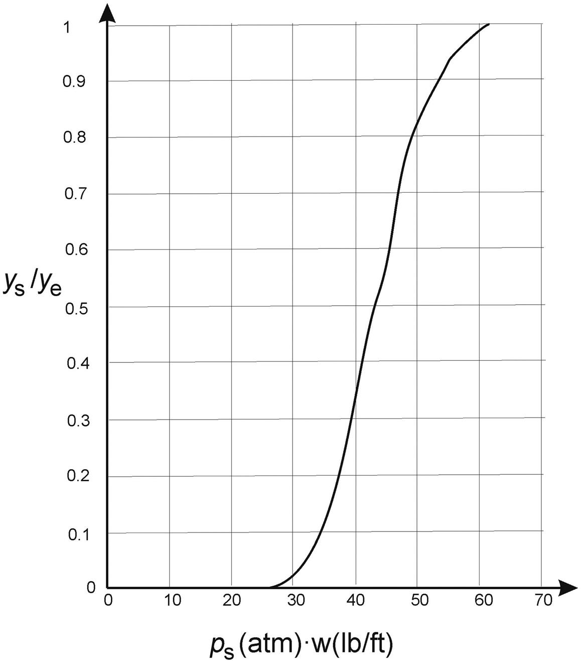
Atmospheric air at 25°C and φ=0.85 is processed using an adsorbent bed to maintain the relative humidity of the product at 0.25. The total gas flow is 45 m3/min. The desiccant bed is made of silica gel and its dimensions are 15 inches (height) by 5 feet (radius). The adsorption capacity can be seen in Fig. 3E13.1. Compute the fraction of air bypassed as a function of time, and how long the bed can be in operation before regeneration.
Solution
Fig. 3E13.2 presents a scheme of the operation. We used the following notation:
ys: Air specific moisture exiting the bed (kg/kgdry air)
ye: Air specific moisture fed to the bed (kg/kgdry air)
yf: Air specific moisture required (kg/kgdry air)
We compute the specific humidity entering, ye, and that required for the product air, yf:
We perform a mass balance to water where x is the bypassed fraction of the initial stream:
The mass flow is given as follows:

The fraction bypassed changes with time, and therefore not only x, but also the humidity of the air exiting the bed is as follows:


Thus for pressures at the bed, the ratio ys/ye is computed. With that, at different time intervals we average the humidity and compute the bypassed fraction. Discretizing the differential equation, the time is determined (see Table 3E13.1). Fig. 3E13.3 shows the profile of the evolution of the bypass fraction and the specific moisture exiting the bed:
Table 3E13.1
Results of the Discretized Operation of the Adsorbent Bed
| Psatw | w | ys/ye | ys | DW | ymed | x | Dt | t | y | x |
| 0 | 0 | 0 | 0 | 1008.1691 | 0 | 0.42222222 | 1194 | 0 | 0 | 0.42222222 |
| 28 | 1008 | 0 | 0 | 72.0120789 | 0.0001499 | 0.41737011 | 85 | 1193.92208 | 0 | 0.42222222 |
| 30 | 1080 | 0.02 | 0.00029981 | 144.024158 | 0.00089942 | 0.39183354 | 162 | 1278.49202 | 0.00029981 | 0.41737011 |
| 34 | 1224 | 0.1 | 0.00149903 | 108.018118 | 0.00224855 | 0.33974346 | 112 | 1440.52981 | 0.00149903 | 0.39183354 |
| 37 | 1332 | 0.2 | 0.00299806 | 108.018118 | 0.00374758 | 0.27029946 | 101 | 1552.47033 | 0.00299806 | 0.33974346 |
| 40 | 1440 | 0.3 | 0.00449709 | 0 | 1653.75772 | 0.00449709 | 0.27029946 | |||
| 0 | ||||||||||
| 1654 |


3.5 Problems
P3.1. In a Linde-type liquefaction process, air is compressed to 100 atm and expanded to 1 atm. The liquid fraction is 0.0385 kg/kg. Assuming that the heat loss is 0.313 kcal/kg and the temperature difference in the hot end of the heat exchanger is 2.8°C, compute the temperature of the compressed air before expansion.
P3.2. Air is liquefied using a modified Linde-type cycle. Atmospheric air at 80.6°F is compressed up to 100 atm. It is cooled down using the nonliquefied fraction and expanded isentropically to 1 atm, separating the gas and liquid phases. The liquefied fraction is 0.28 and the flowrate of air 0.83 ft3/s, measured at 1 atm, and 60°F, determine:
1. The temperature of the cold extreme of the heat exchanger assuming that the energy losses of the system are 40 BTU per kmol of fed air. The ΔT in the hot stream is 5°F.
2. The energy required by the compressor, as well as that produced in the expansion.
P3.3. Atmospheric air is liquefied using a process as in Fig. P3.3. Air at 27°C and 1 atm is compressed using 538.7 kJ/kg of initial air in a compressor whose efficiency is 80%. The compressed air is cooled down at constant pressure with the nonliquefied air. Next, it is expanded isenthalpically to obtain a liquid fraction of 0.05. Assume that all the heat losses take place in the heat exchanger. Compute the pressure of the air at the hot extreme of the heat exchanger (P1), the temperature of the nonliquefied air (T4), and the energy loss per kg of atmospheric air.
P3.4. Determine the liquid fraction of a process such as in Fig. P3.4, considering two isenthalpic expansions. The first one expands the air to 20 atm at 60 kcal/kg of enthalpy, and then the liquid fraction is further expanded to 1 atm.
P3.5. A flowrate of 1000 ft3/min of air at 70°F and 80% moisture is to be processed and fed to a facility with only 10% moisture. Silica gel is used as the absorbent bed (see Fig. P3.5). Part of the initial feed is bypassed dynamically so that the final moisture is controlled. The vessel diameter can be up to 5 ft and the operating time before regeneration must be 3 h. Assuming isothermal operation, determine the bed diameter and its depth. The absorption capacity can be seen in the figure.
P3.6. A Claude-type cycle is used to liquefy air originally at 1 atm and 300K. It is expected that the system recovers 10% of the compression energy that has compressed the air up to 80 atm. Fifty percent (50%) of the initial stream is sent to the expansion machine. Assume that the heat loss of the system is 6 kcal/kg of the initial processes air and that the nonliquefied fraction exits the system 3°C below the initial temperature. Determine:
3. And compare the system to another one that compress the air up to 200 atm, assuming net losses of 6 kcal/kg and that the air exits at 297K.
P3.7. The technical department has received three alternatives for the liquefaction of air. Atmospheric air at 1 atm and 27°C is fed to each one and the nonliquefied fraction exits the system at 24°C and 1 atm. System I is a nonideal Linde cycle, while systems II and III use different refrigerants before expansion. Which one will you recommend to the CEO (Table P3.7)?
P3.8. Air is liquefied using a modified Linde cycle with two consecutive compression stages, the first one from 1 to 20 atm, and the second one from 20 to 150 atm (see Fig. P3.8). The compressed air is cooled down with nonliquefied fractions. The cold air is expanded from 150 atm to 20 atm, and after being used to cool down compressed air, recycled before the second compression stage. The mixture of both streams is at 25°C. The liquid air at 20 atm is expanded to 1 atm. Determine the liquid fraction and the work required at each stage per kg of initial air.
P3.9. The technical department receives the task of suggesting a system to liquefy air using only one expansion stage so that if the heat losses are 3 kcal/kg of initial air, it allows production of a liquid fraction of at least 15%. Initial air is at 27°C and 1 atm, and the nonliquefied fraction exits the system at 24°C and 1 atm (see Fig. P3.9). Determine the temperature at the inlet of the gas–liquid separator.
P3.10. A simple stripping tower processes partially liquefied air whose liquid fraction is the same as that obtained from a simple Linde system. The Linde system processes atmospheric air at 27°C and 1 atm that is compressed up to 200 atm and operates ideally with no heat loss. The column produces a residue that is 5% molar in nitrogen and obtains 95% of the maximum ideal composition in the distillate. Determine the number of trays and the distillate composition.
P3.11. A Linde cycle with prerefrigeration processes atmospheric air at 27°C and 1 atm. It compresses up to 200 atm. It is expanded to 1 atm and the nonliquefied fraction exits at 24°C. The heat losses in the system are 3 kcal/kg. Three different refrigerants are available. The aim is to obtain a liquid fraction of 0.15 kg per kg of initial air (at least). Each refrigerant has a cost and generates a certain environmental burden. The emission cost for the facility is 50 €/t of CO2. Select the most appropriate refrigerant (Table P3.11).
P3.12. A Linde-type air liquefaction system is used in a certain facility. The energy consumption of the plant is 109 kcal/kg of fed air. The liquefied fraction turns out to be 20% when 15 kcal/kg of refrigeration is used, and 29% when using 25 kcal/kg of refrigeration. Assume that the loss of energy is a constant fraction of the refrigeration. The nonliquid air exits at 290K and 1 atm. Determine the operating pressure and the design pressure of the compressor, and also its efficiency.
P3.13. A simple Linde column is used to produce rich oxygen and nitrogen. Over the top vapor with 85% in nitrogen is obtained. It represents 95% of the maximum concentration possible. From the bottom, a stream with 5% nitrogen is produced. Determine the liquefied fraction of the air fed to the column, a feasible air liquefaction cycle, and the number of trays for the column.
P3.14. Determine the refrigeration needed in a cycle (like the one in Fig. P3.14) to produce 0.3 kg of liquid air per kg of initial feed, assuming that the first expansion is down to 20 atm and the second one to 1 atm.
P3.15. In a Linde simple column system (see Fig. 3.11), air is fed at 300K. It is compressed up to 200 atm. It is cooled down with the gas products N2 and O2, which exit the column at their boiling points of 77K and 90K, respectively, with the system at 127K. Compute the number of trays assuming that the nitrogen purity is 95% of the one corresponding to the thermodynamic equilibrium, and that the oxygen contains 5% nitrogen. Assume that the Hauser diagram (Fig. 3.1) holds for all enthalpy computations.
P3.16. Determine the maximum pressure at which a stream at 10°C and a specific humidity of 0.0045 kgs/kgdryair, and a second stream at 45°C and 0.048 kgs/kgdryair, can be mixed in any proportion with no condensation.


Table P3.7
| I | II | III | |
| Compressed air | 200 atm 300K | 100 atm 300K | 100 atm 300K |
| Heat losses | 2 kcal/kg initial air | – | – |
| Refrigeration | 5 kcal/kg initial air | 8 kcal/kg initial air | |
| Electricity cost | 0.15 €/kWh | 0.15 €/kWh | 0.15 €/kWh |
| Refrigerant costs | – | 0.0025€/kg liq. air produced | 0.004€/kg liq. air produced |
| Environmental impact | 0.02·(W (kcal/kgliquid air))+0.25·(QRefrigeration (kcal/kgliquid air)) | ||
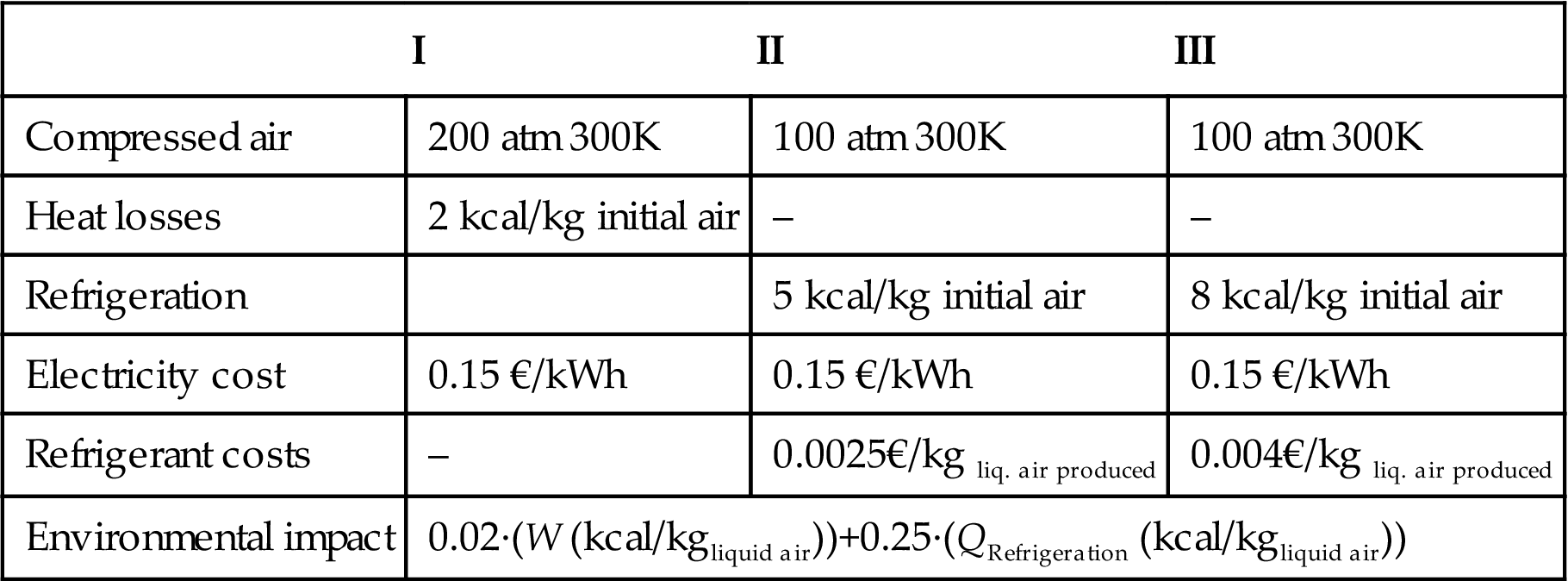
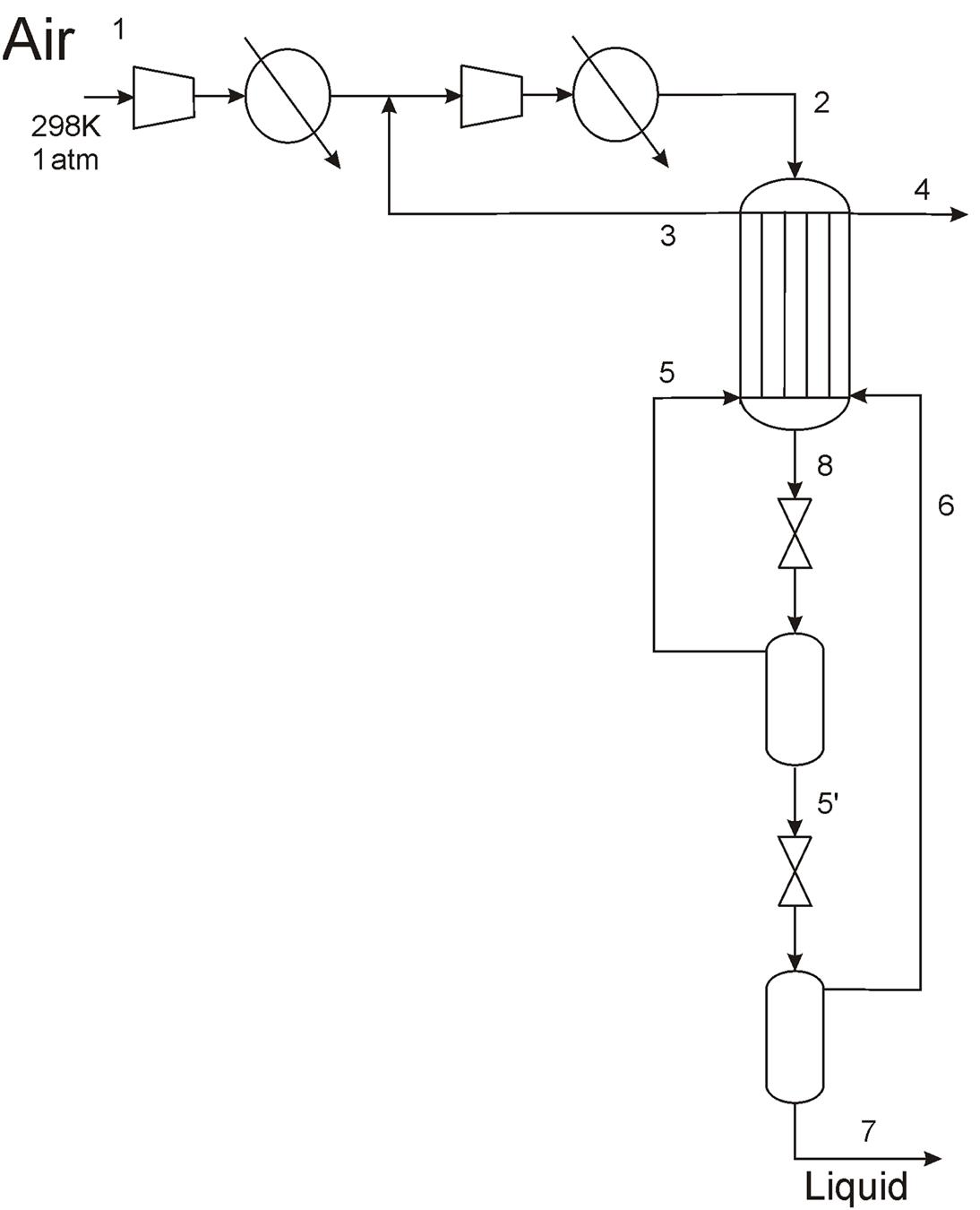

Table P3.11
| I | II | III | |
| Q (kcal/kg initial air) | 15 | 20 | 25 |
| Coste (€/kcal refrigerant) | 4 | 5 | 6 |
| Impact (kg CO2 produced/kcal refrigerant) | 45 | 40 | 20 |

