Keywords

Process synthesis; mass and energy balances; flowsheeting; sustainable and safety design

2.1 Introduction to Process Engineering

The word design refers to a creative process searching for the solution to a particular problem. When it comes to chemical processes, the aim is to come up with the stages and the units that transform a raw material or a number of raw materials into a desired set of products. At this point we must refer to the book by Rudd, Powers, and Siirola (1973), the first one to present this procedure as a systematic process. The field of chemical process engineering finds in that work its first textbook.

A chemical plant or facility comprises a number of operations and reactors that allow the transformation of raw materials into products of interest and their purification. The typical stages are as follows:

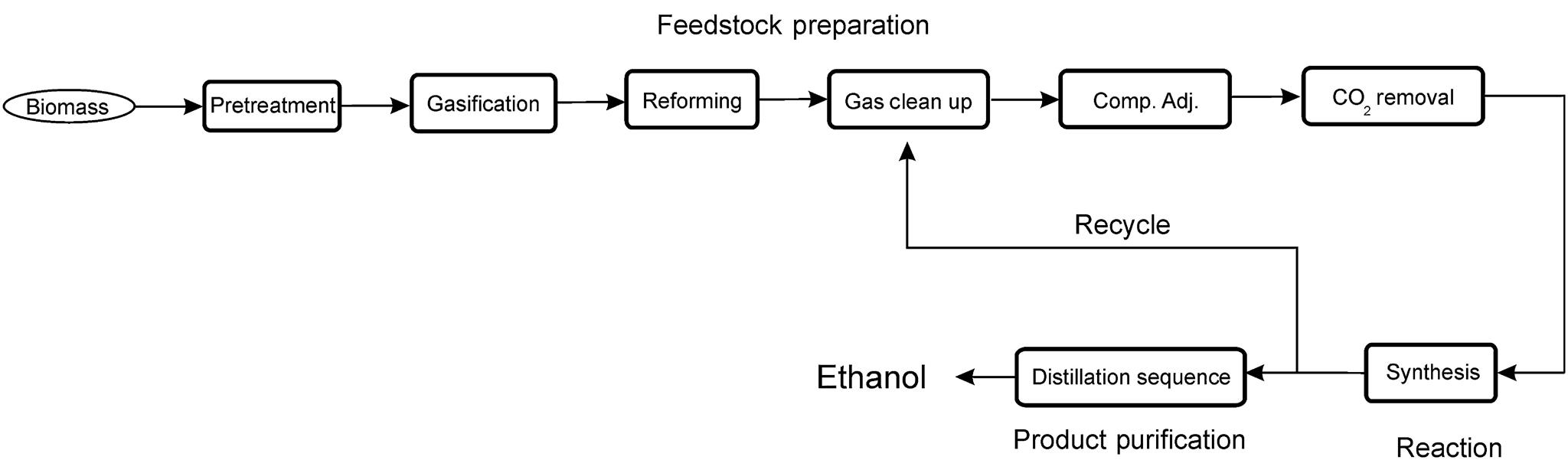
In Fig. 2.1 we present the scheme for the production of ethanol via biomass gasification. We see the different stages of any chemical process. Biomass is processed so that the size is appropriate for gasification. Next, the raw syngas is purified from hydrocarbons, hydrogen sulfide (H₂S), ammonia (NH₃), etc., and its composition adjusted in terms of the hydrogen (H₂) to carbon monoxide (CO) ratio. Subsequently, the gas reacts to produce not only the desired product, ethanol, but also methanol, propanol, and butanol. Furthermore, the conversion of the syngas is not complete, and the unreacted gases are separated and recycled, while the liquid products are separated via distillation. This process also has emission control units in the form of sour gas capture. Carbon dioxide (CO₂) and H₂S are removed from the gas stream because they are poisonous for the catalyst.

The process engineer is the person responsible for putting together the flowsheet that defines the path from the raw materials to the products. His main aim is to find the optimal way to obtain a product with the specifications that meet the demand at the lowest cost, under safe conditions, and with the lowest environmental impact. Therefore, process optimization has an important role. Before 1958, the good economic situation allowed a number of rules that resulted in units being overdesigned. In addition, environmental constraints were relaxed to help grow the economy. However, as times became tougher, the processes were designed and operated closer to their optimal specifications. Therefore, the process engineer had a more difficult task. Nowadays, overdesign is a burden for the profitability of the facility.

Making decisions on the best process is a tough problem in itself. First, there are multiple alternatives for almost every processing stage. Furthermore, there is no single design criterion, but a number of them. Economic evaluation is the one every manager will ask for first. However, society is concerned with the environment and the security of the people that work in the plant and close by. Therefore, environmental assessment, safe operation, and flexibility are other concerns that transform the original problem into a multiobjective one.

There are four main problems that the process engineer typically has to address:

The project consists basically of deciding:

The process engineer must consider all of these aspects when dealing with a process. Process design can be divided into four stages.

2.2 Principles of Process Design

In this section we present to the reader methods to sketch the flow diagram for a process. Some of the methods will not be further pursued in this text, but it is important that the reader becomes acquainted with the words and terms in process design. All these methods aim to propose a systematic way of evaluating the large number of alternatives that the process engineer has to consider in order to come up with a process flowsheet.

A. Hierarchy Decomposition

In this method, proposed by Douglas in 1985 and later modified by R. Smith at the University of Manchester (UMIST by that time) (Smith, 2005), there are five decision levels.

B. Superstructure Optimization

This method consists of the formulation of a mathematical problem where all the alternative processes are modeled based on mass and energy balances, thermodynamic equilibrium, rules of thumb, experimental data, etc. The optimal flowsheet is extracted from the superstructure by solving the problem. For further details see Biegler et al. (1997), Kravanja and Grossmann (1990), and Yeomans and Grossmann (1999).

C. Evolutionary Methods

These are based on know-how and a previously available design. Using the original process as a starting point, it is modified to address its weaknesses and/or to increase capacity.

In order to the reader to have a better understanding of the processes that will be described in the following chapters, we are going to briefly comment on the first of the three methods. However, in some processes (eg, air liquefaction, lead chambers), evolutionary methods are behind the development of alternatives for improving the yield, as it will be shown in the following chapters.

2.2.1 Douglas hierarchy (Douglas, 1988)

2.2.1.1 Level 1: batch versus continuous process

We use a batch process under the following circumstances:

• Low production capacity (typically below 5×10⁵ kg/y).

• Multiproduct plants (eg, cosmetics and detergents).

• Special market properties such as seasonality (eg, ice cream and buñuelos) or aging (eg, fresh food).

• When there are scale-up problems. For instance, in batch exothermic reactions, the larger volumes do not maintain the area-to-volume ratio, and heat transfer problems may appear.

2.2.1.2 Level 2: input–output structure

At this level we try to answer a number of questions related to the purity of the raw material: Should we purify them? The purity of the byproducts: Should we recycle or eliminate them? Do we need to purge part of the recycle to avoid build-up within the process? Furthermore, can the unreacted raw materials be recycled or not? We also need to evaluate the number of product streams of the process. Based on this black box analysis of the process, the preliminary economic potential of the alternatives can be determined in order to disregard the worst ones. To address all of these questions there are some basic rules:

• If the impurity is not inert, we need to remove it.

• If the impurity is in the feedstock and it is in the gas phase, we process it.

• If the impurity is in a liquid feedstock and it is a product or a byproduct, we process the feedstock though a separation stage.

• An impurity in large amount must be removed.

• If the impurity is an azeotrope, we process it.

• We must determine when it is easier/cheaper to eliminate the impurity from the feedstock or from the products.

• If the boiling point of the impurity is lower than −48°C, we need to purge it or use membrane separation.

• Oxygen, water, or air are used in excess as reactants.

• The number of product streams depends on the boiling point of the gases and liquids that we obtain. Solids are evaluated separately.

• Valuable byproducts are sold.

• Avoid buildup in the process.

2.2.1.3 Level 3: recycle

This decision level is used to evaluate the reaction step. The aim is to determine the reaction steps required, the recycle streams, and the need for an excess of one of the reactants. For that we need to know the kinetics and equilibrium governing the chemical reaction or reactions in order to figure out how it/they can be altered. Typically the reactions involve heat transfer, and sometimes the design of the reactor is heavily conditioned by how we can remove the heat generated. The effect of the reaction on the economic potential is addressed at this level.

Apart from know-how on the reaction step, a set of general rules can also help in decision-making:

• There exist optimal conditions for the operation of the reactor in terms of feedstock composition, pressure and temperature, and reactor configuration for heat removal as a result of the chemical reaction or reactions taking place.

• If there are several reactions that require different operating conditions, a number of reactors are needed.

• If the reaction is exothermic, but the increase in the temperature is lower than 10%, the reaction operates as adiabatic.

• For an endothermic reaction, heat can be provided directly for isothermal operation and low production capacity, or indirectly for higher production capacity.

• The aim is to reach 96–98% of the equilibrium conversion.

2.2.1.4 Level 4: separation structure

From this point on, the separation costs are included in the evaluation. The product stream from the reactor is evaluated as follows:

• If it is in the liquid phase, the separation is based on species volatility. If the relative volatility is larger than 1.1, distillation is selected, otherwise liquid–liquid separations can be considered.

• If we have a gas–liquid mixture, a flash separation is used to separate phases.

• If the reactor operates at high temperature, the products are cooled down and condensed. If the cooled liquid phase comprises only reactants, it is recycled. If it contains only products, it is sent to further purification. The gas phase is sent to vapor recovery. The reactants are recycled. We can avoid flash separation if the amount of vapor is small. In that case the multiphase stream is sent to liquid separation.

• If the product is in the vapor phase, the stream is cooled down to condense a fraction and separate the phases. The condensed liquid is processed as described above. Sometimes cooling is not enough and compression can be used to separate the phases. Otherwise, if the phases cannot be separated, partial condensation is considered.

• If the products in a stream have no value, the stream is not further processed.

Another method is the one proposed by Jaksland et al. (1995), which consists of two levels. In the first level, the mixture is characterized to identify the separation technique based on the vapor pressure ratio. In level two, we select the separation task, the sequence of separations, and determine the need for solvent and type.

In this stage we see that distillation is the most important operation to separate liquid mixtures. Distillation is an energy-intense operation. When a mixture of components is to be separated, the order of their separation determines the cost of the product. Therefore, much effort has been placed on systematically determining the cheapest distillation sequence. There are two main approaches: heuristic rules and mathematical optimization. For the sake of this text we focus on the first one and leave the reader with the reference for the second (Biegler et al., 1997).

Synthesis of distillation sequences (Rudd et al., 1973, Jiménez, 2003)

Relative volatility, of the species involved determine the separation of the mixture. If it is 1, there is no way. If it is 1–1.1, it is difficult. If it is 1.1 or higher, it is easy. Thus, if the relative volatility of two species is lower than 1.1, distillation is not an option.

The problem we face here is the large number of options; for example, for three components, assuming sharp splits, there are two different flowsheets:

$\begin{array}{c}(\mathrm{ABC})-[(\mathrm{A})-(\mathrm{BC})]-[(\mathrm{B})-(\mathrm{C})]\\ (\mathrm{ABC})-[(\mathrm{AB})-(\mathrm{C})]-[(\mathrm{A})-(\mathrm{B})]\end{array}$

For four components we get five flowsheets. In general, let N be the number of components; the number of units, N_o, is given as

$N_{\mathrm{o}}=\frac{[2(N-1)]!}{(N-1)!N!}$ (2.1)

(2.1)

For a one distillate–one bottom column, the general rules are as follows:

1. Remove corrosive or reacting component first.

2. Remove products as distillates.

Heuristics for Column Sequencing

H1. Forbidden splits:

a. Don’t use distillation if the relative volatility is lower than 1.05.

b. If (α−1)_{extractive dist.}/(α−1)_{reg. distillation} <5, use ordinary distillation.

c. If (α−1)_{sep liq–liq}/(α−1)_{reg. distillation} <12, use ordinary distillation.

d. Consider absorption as a candidate if refrigeration is needed for distillation.

H2. The next separation is that with the largest relative volatility. Easy first, difficult last.
This rule is based on the size of the column. The minimum number of stages in a distillation column can be computed as given by Eq. (2.2):

$N_{\min }=\frac{\log \left[\left(\frac{x_{i,D}}{1-x_{i,D}}\right)\left(\frac{1-x_{j,W}}{x_{j,W}}\right)\right]}{\log {\alpha }_{ij}}$ (2.2)

(2.2)

where α is the relative volatility, and x_i is the molar fraction of component i in the feed, F, or the distillate, D. Therefore, the larger the relative volatility, the shorter the column.

H3. Remove the most abundant component first.
The size of the column (its diameter) is a function of the vapor phase across it as given by Eq. (2.3), where V is the vapor flow and u the vapor velocity across the column, ρ the density, and K the design constant:

$D=\sqrt{\frac{4V({\mathrm{m}}^3/s)}{\pi u(m/s)}}=\sqrt{\frac{4V({\mathrm{m}}^3/s)}{\pi K\sqrt{\frac{{\rho }_{\mathrm{L}}-{\rho }_{\mathrm{V}}}{{\rho }_{\mathrm{L}}}}}}$ (2.3)

(2.3)

Furthermore, the flowrate of the vapor phase has to be reboiled. Thus, the energy at the reboiler increases for higher flowrate. If we reduce the flow processed in the column by separating the most abundant sooner, the following columns will be smaller and the energy consumption lower.

H4. If the α and concentration are not very different, use direct sequence (most volatile first).
The justification behind this rule is again related to the energy consumption and the diameter of the column. Let’s assume a mixture ABC equimolecular with similar relative volatilities between the components AB and BC, and that the feed is saturated liquid.
Direct Separation: See Fig. 2.2 for the flow pattern across the column.
Indirect Separation: See Fig. 2.3 for the flow pattern across the column.
Therefore, the direct sequence is cheaper.

H5. Remove mass separation agent in the next column.

H6. Favor sequences that do not break desired products. We save a column or more.
These rules must be applied in order of priority, and every time a decision on the separation of products is to be made.

Example 2.1

Let’s look at an example for the separation of a mixture courtesy of Prof. I.E. Grossmann. Fig. 2E1.1 presents an example for the use of the heuristic rules.

The order for the volatilities of the species and the values are given below:

$\begin{array}{ll}\mathrm{O}(\mathrm{I})\hfill & :\text{ABCDEF}\hfill \\ \mathrm{O}(\mathrm{II})\hfill & :\text{ACBDEF}\hfill \\ \hfill & {\alpha }_{\mathrm{I}}\mathrm{A}/\mathrm{B}2.45,\mathrm{B}/\mathrm{C}1.18,\mathrm{C}/\mathrm{D}1.03,\mathrm{E}/\mathrm{F}2.5\hfill \\ \hfill & {\alpha }_{\mathrm{II}}\mathrm{C}/\mathrm{B}1.17,\mathrm{C}/\mathrm{D}1.7\hfill \end{array}$

Solution

H1. Exclude (C/D)_Ι since α_Ι=1.03

${(\mathrm{B}/\mathrm{C})}_{\mathrm{{\rm I}}}1.18\mathrm{vs}{(\mathrm{C}/\mathrm{B})}_{\mathrm{{\rm I}}\mathrm{{\rm I}}}1.170.18/0.17<5\to \mathrm{exclude}{(\mathrm{C}/\mathrm{B})}_{\mathrm{{\rm I}}\mathrm{{\rm I}}}$

H2. Separate largest α

${\alpha }_{\mathrm{{\rm I}}(\mathrm{{\rm A}}/\mathrm{B})}2.45.$

Similarly,

${\alpha }_{\mathrm{{\rm I}}(\mathrm{E}/\mathrm{F})}2.5$

H3. Get rid of most abundant

$\mathrm{A}/\mathrm{B}=5\mathrm{A}\mathrm{E}/\mathrm{F}=12\mathrm{F}$

Small amounts.

H4. Direct sequence favors → (A/B)_I

The desired products are BDE & C (Fig. 2E1.2).

1. We can separate C/BDE using extractive distillation. However, H1 does not recommend the use of extractive distillation.

2. We can separate BC/DE. Again, H1 does not recommend the use of regular distillation since the relative volatility is lower than 1.05.

3. We separate B/CDE using regular distillation (α=1.18).
Next, we separate C/DE using extractive distillation (α=1.7):

$\frac{{(\alpha -1)}_{\mathrm{II}}}{{(\alpha -1)}_{\mathrm{I}}}=\frac{1.7-1}{1.03-1}\ge 5$

We mix B and (DE)

Example 2.2

We have a mixture of propane (45.4 kmol/h), isobutane, (136.1 kmol/h), n-butane (226.8 kmol/h), i-pentane (181.4 kmol/h), and n-pentane (317.4 kmol/h) with relative volatilities of C₃/iC₄=3.6, iC₄/nC₄=1.5, nC₄/iC₅=2.8, iC₅/nC₅=1.35. Determine the sequence of distillation columns to separate the mixture.

Solution

Using H2 we separate (C₃|iC₄ nC₄ iC₅ nC₅).

Using H2 we separate (iC₄ nC₄|iC₅ nC₅).

Using H2 we separate (iC₄|nC₄) (iC₅|nC₅).

2.2.1.5 Level 5: heat recovery and integration

Hierarchy decomposition considers heat integration as the last stage in process design. However, energy consumption represents one of the major economic burdens of any process, and therefore energy integration must be considered along with process synthesis. In fact, at Level 3 we already considered the operation of the reaction involving heat transfer. The aim of this stage is to identify the sources of energy within our process and reuse it in a systematic way. We consider two cases for heat integration due to their impact on the economy of the processes: the heat exchanger networks (HENs), to determine the minimum utility cost; and in the second step the design the structure of the network and multieffect columns, which have proved to be extremely useful to reduce energy consumption in bioethanol production processes.

Heat exchanger networks

Utilities Minimization

Given:

• a set of hot streams that require cooling and a set of cold streams that need energy,

• flowrates and inlet/outlet temperatures are known,

• heat capacities are assumed constant,

• and the utility streams are known,

we aim to design the HEN that minimizes the operating and capital costs. Let us illustrate with an example.

Example 2.3

Design a HEN with minimum consumption of utilities for the stream in Table 2E3.1.

Table 2E3.1

Data for Example 2.3

Streams	Fcp (kW/°C)	Tin (°C)	Tout (°C)	Heat Flow (kW)
C1	15	360	600
C2	13	300	450	5550
H1	10	600	320
H2	20	540	320	7200
				−1650

From the first law of thermodynamics, we need 1650 kW of cooling. However, it is not possible to find a network with 1650 kW (see Fig. 2E3.1).

The procedure for computing the minimum utilities required is as follows:

1. Create temperature intervals. Assume a minimum ΔT_min (HRAT–heat recovery approach temperature), for instance, 10°C. For cold streams, there must be a stream that is at least T+ΔT_min above; ie, for the stream at 260°C, there should be another stream at 270°C. For hot streams, in order to cool them down, we need a stream 10°C below; ie, for the 93°C stream, we need another stream at 83°C.

2. Compute the heat available at each interval, k, and that required. $Q_k=\sum _{i\in \mathrm{cold\; or\; hot}}{F}_i\cdot c_{p,i}\cdot \mathrm{\Delta }{T}_k$

3. Accumulate the heat available and that required; they are the cascades of hot and cold streams. $Q_{\mathrm{available}}={\sum _k{Q}_k|}_{\mathrm{hot}};Q_{\mathrm{required}}={\sum _k{Q}_k|}_{\mathrm{cold}};$

4. Plot the cascades (see Fig. 2E3.1). The change in curvature is given when a second stream contributes to the composite hot and cold curves, respectively. In the figure it is possible to compute the minimum needs for utilities as the difference in the extremes of the curves when they touch. The required energy and the refrigeration needed are computed when both curves are at DT difference. To compute this point we continue the procedure.

5. Determine the Composite Curve (GCC) by accumulating the net energy at each interval k. The minimum value (most negative) is the energy required. By adding this value to the GCC on top we find the required energy, and at the bottom the cooling needs. Table 2E3.2 shows the results for the pinch.
The minimum utilities required are computed when the hot and cold composites are put close so that the distance between them is ΔT_min. Fig. 2E3.2 shows this point. We have horizontally displaced one of the curves so that the hot composite is above the cold one and the distance between them at the closest point in the y axis, the pinch, is ΔT_min. The horizontal distance at the top and at the bottom of the curves gives the minimum heat to be provided and the minimum energy to be removed from the system.

Table 2E3.2

Pinch Example 2.3 Results

Source: Courtesy of Prof. I.E. Grossmann.

HEN Structure

The idea is to minimize the area and the energy to be removed and that provided. Thus, a few heuristics that can be used are the following:

• High temperature streams are integrated first.

• Streams with high heat loads are integrated next.

• Search for larger gradients of temperatures.

• Look for larger global heat transfer coefficients.

Extreme alternatives:

a. Every hot stream with a cooling utility;

b. Every cold stream with a heating utility.

c. Recover as much heat as possible using the least amount of utilities;

Usually, there are many alternatives.

Near optimal HEN usually exhibits:

a. Minimum utility cost for a given DT_min (HRAT+10K).

b. Fewest number of units.

Targeting (Pinch analysis) method:

1. Predict (a) and (b).

2. Develop a network that satisfies (a) and (b).

a. As presented in the previous point

For maximum heat exchange, place curves as close as possible within ΔT_min+HRAT. Note:

HRAT=20K	600 kW heating	2250 kW cooling
HRAT=10K	450 kW heating	2100 kW cooling
HRAT=5K	375 kW heating	2025 kW cooling
HRAT=0K	300 kW heating	1950 kW cooling (Absolute minimum)

1. Determine the excess or need of energy in each interval.

2. Cascade heat with 0 kW heating.

3. Cascade minimum heating:

a. Minimum cooling.

b. Temperature below zero entry-pinch,

Note that there will not be heat transfer across the pinch and we can divide the network into two above and below the pinch,

In the problem table we see that the maximum deficit of energy is 600 kW, which is the energy that needs to be provided.

b. Minimum number of heat exchangers (N_min)

For each subnetwork assume at least one stream is exhausted in each match.

According to Euler’s theorem, for n nodes:

${\mathrm{N}}_{\min }=n(\mathrm{hot})+n(\mathrm{cold})+n(\mathrm{utilities})-1$

The following example illustrates this procedure:

Example 2.4

Design a heat exchanger network (HEN) for the streams in Example 2.3.

Solution

In our case

Streams Above Pinch: H1, C1, steam	Nmin=1+1+1−1=2
Stream Below Pinch: H1, H2, C1, C2, cooling water	Nmin=2+2+1−1=4
	Total=6

• We are looking for a network with 600 kW of heating and 2250 kW of cooling with the pinch at 540–520K.

• It should also have six units (two above the pinch and four below).

The subnetwork above the pinch is shown in Fig. 2E4.1.

Below the pinch, we have several alternatives. Fig. 2E4.2 shows the subnetworks where H2 and H1 are used to heat up C1 and C2, respectively.

However, if we try to use H2 to heat up C1, we have temperature cross.

Thus, the final network is of the form shown in Fig. 2E4.3.

The matches diagram is given by Fig. 2E4.4. We plot the hot and cold streams as lines assuming that the temperature decreases to the right. The matches are represented by lines connecting the streams that exchange energy. We place heat exchangers to represent the heat provided or removed using utilities.

Source: Courtesy of Prof. I.E. Grossmann.

Multieffect columns

In the case of the production of ethanol from corn grain, one of the most energy consuming pieces of equipment is the distillation column known as a “Beer column.” It contributes to almost 50% of the energy of the process. Using multieffect columns the energy consumption is reduced by nearly half, and the cooling needs are also reduced. The operation of the system of columns consists of treating the feed at different pressures so that the boiler of the low-pressure column acts as a condenser for the high-pressure column. The variables are the operating pressures of the columns as well as the fraction of the feed (α_i) that goes to each one of the columns. We have to make sure that T_Reb > T_Cond + ΔT_min. Fig. 2.4 shows a scheme for a system of two columns operating as multieffect.

The formulation of the problem is given by the mass balance to the initial splitter, the temperature constrains so that heat can be transferred from the reboiler of the lower pressure columns to the condenser of the higher pressure columns, and the energy balances so that the heat exchanged between them matches and the mass and energy balances to each of the columns. A pressure increase from the lower pressure column to the higher pressure columns is enforced by a constraint (see Eq. 2.4).

Karuppiah et al. (2008) used this technology in the production of ethanol from corn, resulting in $3 million savings in steam just in the columns (see Fig. 2.5).

$\begin{array}{l}F=\sum _k{F}_k\hfill \\ T{b}_k\le T{c}_{k+1}+dt,k\in \mathrm{COL}\hfill \\ T{b}_k\le T{c}_k+dt,k\in \mathrm{COL}\hfill \\ Q{b}_k=Q{w}_{k+1}\hfill \\ P_{k+1}\ge P_k\hfill \\ M\&E_k\hfill \end{array}$ (2.4)

(2.4)

2.3 Flow Diagrams

2.3.1 Types

Flow diagrams are a way to present information from the process Westerberg et al. (1979). Depending on the audience they are intended for, different formats and standards are applied.

1. Process diagrams.
They are simple representations of the process with no technical details. Their aim is diverse, from publicity and advertising to providing a technical sketch.

a. Block flow diagrams. They consist of a number of boxes representing each of the units or groups of units. The boxes are connected through arrows. See Fig. 2.6.

b. Block flow process diagram. It is used for simple representation of the entire process. Typically all the units of the process are represented and linked by arrows, indicating the direction of the flow. Some major operating conditions are added to highlight them. It is the basis for the engineering process diagrams. See Fig. 2.7.

c. Graphic process diagram. It is widely used in publicity or to sell the project to managers. It is free, and they are not standardized. See Fig. 2.8.

d. Sankey diagram: It shows the flow of energy or mass involved in the process, typically as a whole. It allows identifying energy losses. See Fig. 2.9.

2. Process flow diagrams. They are the major source of information regarding a process, from the stream data to equipment sizing. The symbols that are used for the units and the way of reporting information on the operating conditions are standarized. Anyone in the field can interpret the diagram (see Fig. 2.10). The information on the streams must be provided here. See Section 2.4 for a detailed list of variables. A special type of engineering process diagram is the so-called Piping and Instrumentation Diagram. It includes everything from the size of the pipes and their material to the controllers and measuring devices needed for controlling the operation of the facility (see Fig. 2.11). Within the flag for a controller, the variable that is being measured and the action are reported using a legend. Typically there is a system of three letters XYY; Table 2.1 shows these letters.

Table 2.1

Letters for Instrumentation

	First Letter (X)	Second or Third Letter (Y)
A	Analysis	Alarm
B	Burner flame
C	Conductivity	Control
D	Density or specific gravity
E	Voltage	Element
F	Flowrate
H	Hand	High
I	Current	Indicate
J	Power
K	Time or time schedule	Control station
L	Level	Light or low
M	Moisture or humidity	Middle or intermediate
O		Orifice
P	Pressure or vacuum	Point
Q	Quantity or event
R	Radioactivity or ratio	Record or point
S	Speed or frequency	Switch
T	Temperature	Transit
V	Viscosity	Valve, damper, louver
W	Weight	Well
Y		Relay or compute
Z	Position	Drive

In this special diagram the information related to the equipment is provided. For instance, we need to describe the units in parallel or the spare units that are needed in the process. With respect to the units, we provide the size, the thickness (Schedule) of the pipes and the equipment, the materials of construction and the isolation, type, and thickness. In Table 2.2 the typical operating information for the units reported in the diagrams is known. We also need to provide control information such as indicators, controllers, recorders, etc. Finally, the utilities used in the process must be provided.

Table 2.2

Typical Information Displayed

Unit	Information
Towers	Size (height and diameter), pressure, temperature Number and type of trays Height and type of packing Materials of construction
Heat exchangers	Type: gas–gas, gas–liquid, liquid–liquid, condenser, vaporizer Process: duty, area, temperature, and pressure for both streams Number of shell and tube passes Materials of construction: tubes and shell
Vessels and tanks	Height, diameter, orientation, pressure, temperature, materials of construction
Pumps	Flow, discharge pressure, temperature, ΔP, driver type, shaft power, materials of construction
Compressors	Actual inlet flow rate, temperature, pressure, driver type, shaft power, materials of construction
Fired heaters	Type, tube pressure, tube temperature, duty, fuel, material of construction

2.3.2 Symbols: Process Flowsheeting

Each of the units involved in a process flowsheet has its symbol. Fig. 2.12 shows the symbols for a number of typical equipment types. The units are referred to using their initials, such as C for compressors and turbines, E for heat exchangers, H for fire heaters, P for pumps, R for reactors, T for towers, TK for storage tank, V for vessels, and also a number, since typically there are various units of the same category in the plant.

Control instrumentation and the values provided in the flowsheet legend to report a flow rate using different units, mass or molar, pressure and temperature, etc. Fig. 2.13 shows the classic symbols for the control equipment, with lines representing the types of signals and flags for the information on the diagram.

2.4 Mass and Energy Balances Review

Mass and energy balances must provide the information for the streams displayed in the diagrams presented in Section 2.3. Typically the following information is to be included:

Sometimes there is an error in the global mass balance, especially if there are experimental data or correlations used to perform the balances. There is a maximum: even if the balances hold, it does not mean that they are correct. Finally, the presentation of the results must accurately display the number of significant digits. There are two approaches to performing the mass and energy balances for a facility: equation-based and modular. The first one is the option of choice in most of this text, and a review of the principles is provided below. However, the use of computers in chemical engineering has spread, and modular simulators have been developed, such as CHEMCAD or ASPEN. For an introduction to the use of software for solving chemical engineering problems, we refer the reader to Martín (2014).

2.4.1 Equation-Based Approach

The model for each unit and for the process itself comprises all the first principle equations that govern the system. It is out of the scope of this book to provide a detailed review of the principle chemical processes, those of unit operations or chemical reaction engineering; other books are better suited for this. Here we only present a brief review of the principles that will be used for the calculations in this book. We refer the reader to specific literature for further information (Houghen et al., 1959; Baasel, 1989; Walas, 1990; Fogler, 1997; Perry and Green, 1997; McCabe et al., 2001; Seider et al., 2004; Towler and Sinnot, 2012).

2.4.1.1 Mass and energy balances

They are based on the thermodynamic principles of conservation:

Mass balance with no chemical reaction, ie, mixers, separators, heat exchangers:

Mixer, heat exchanger,

$\sum _{i\in \mathrm{inlet}}{m}_{i,j}=m_{\mathrm{out},j}\forall j$ (2.5)

(2.5)

Splitter,

$\begin{array}{ll}{m}_{\mathrm{out}-k,j}\hfill & =({\xi }_k)m_{\mathrm{in},j}\forall j\hfill \\ \sum _k{\xi }_k\hfill & =1\hfill \end{array}$ (2.6)

(2.6)

Mass balance with chemical reaction

a. Elementary balance:

$\sum _{\mathrm{in}}{n}_i=\sum _{\mathrm{out}}{n}_i$ (2.7)

(2.7)

b. Stoichiometry:

$aA+bB\to cC+dD\begin{array}{cc}{n}_{\mathrm{A}}& =n_{\mathrm{A},\mathrm{ini}}-a/a·n_{\mathrm{A},\mathrm{ini}}·X\\ n_{\mathrm{C}}& =n_{\mathrm{C},\mathrm{ini}}+\frac{c}{a}{n}_{\mathrm{A},\mathrm{ini}}·X\end{array}$ (2.8)

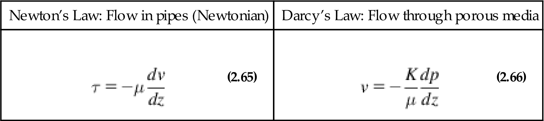
(2.8)

where X is the conversion for the reaction. We define conversion as the fraction of the limiting reagent that has reacted. The reagent in excess is defined with respect to the stoichiometry of the reaction and the limiting reagent. Selectivity, S, refers to the fraction of the converted reagent that produces a certain product in multiple reaction systems.

c. Electrochemical reactions:

Redox potential:

$E_{\mathrm{Reaction}}=E_{\mathrm{semi}\_\mathrm{reduction}}-E_{\mathrm{semi}\_\mathrm{oxidation}};E>0\mathrm{Spontaneous}$ (2.9)

(2.9)

Nerst equation:

$E=E°-\frac{R·T}{n·F}·\ln \left[Q\right]$ (2.10)

(2.10)

Power:

$e·F·V\equiv I·t·V$ (2.11)

(2.11)

Charge flow:

$e·F\equiv I·t$ (2.12)

(2.12)

Equivalencies:

$1\mathrm{C}=1\mathrm{A}\cdot \mathrm{s};\mathrm{F}=\mathrm{C}/\mathrm{mol};1\mathrm{C}=\mathrm{V}\cdot \mathrm{F},\mathrm{V}=\mathrm{J}/\mathrm{C}$

2.4.1.2 Energy balances

• Enthalpy diagrams: Mollier, Hausen, enthalpy composition. In these diagrams the Lever rule is useful for computing mixture composition and enthalpies.

• Specific enthalpy (flow enthalpy–sensible heat; we can also correct c_p with pressure):

$H(T)=H_{T_{\mathrm{ref}}}^T=\underset{T_{\mathrm{ref}}}{\overset{T}{\int }}{c}_{p,i}(T)dT=\underset{T_{\mathrm{ref}}}{\overset{T}{\int }}(A+BT+C{T}^2+D{T}^3)dT\approx \overline{c_p}(T-T_{\mathrm{ref}})$ (2.13)

(2.13)

• Enthalpy of reaction:
Heat of formation. We compute it as given by Eqs. (2.14) and (2.15), depending on the aggregation stage of reference of the chemical for gases and liquids, respectively.
Gas:

$\mathrm{\Delta }{H}_{\mathrm{f},T}=(H_T^{T_{\mathrm{ref}}}+\mathrm{\Delta }{H}_{\mathrm{f},T_{\mathrm{ref}}})$ (2.14)

(2.14)

Liquid:

$\mathrm{\Delta }{H}_{\mathrm{f},T}=\lambda (T)+H_{T_{\mathrm{ref}}}^T+\mathrm{\Delta }{H}_{\mathrm{f},T_{\mathrm{ref}}}=c_{p,\mathrm{liq}}(T-T_{\mathrm{ebul}})+\lambda (T_{\mathrm{ebul}})+H_{T_{\mathrm{ref}}}^{T_{\mathrm{ebull}}}+\mathrm{\Delta }{H}_{\mathrm{f},T_{\mathrm{ref}}}$ (2.15)

(2.15)

Enthalpy of mixtures. For acids and alkalis in water we need to consider the energy involved in the dilution or concentration, heat of dilution. However, in most cases heats of mixing are negligible and enthalpies can be considered as additive.
Heat of reaction: Assuming the heat of formation at reference temperature for the species in the final aggregation state, we have the heat of reaction:

$\sum _{j=\mathrm{in}}\sum _i{n}_i{(H_T^{T_{\mathrm{ref}}}+\mathrm{\Delta }{H}_{\mathrm{f},T_{\mathrm{ref}}})}_i+{\text{Q}}_{\text{reaction}}=\sum _{k=\mathrm{out}}\sum _i{n}_i{(H_T^{T_{\mathrm{ref}}}+\mathrm{\Delta }{H}_{\mathrm{f},T_{\mathrm{ref}}})}_i$ (2.16)

(2.16)

To compute the enthalpy of the components, the Hess principle holds (see Fig. 2.14). Alternatively it can be computed using heat of combustion of the species.

• Polytropic compression. We compute the work involved by integrating Eq. (2.17). Typically, a compression ratio not larger than 4 or 5 is used based on rules of thumb.

$W=-\int PdV;P{V}^{\gamma }=cte$ (2.17)

(2.17)

$W(\mathrm{Comp})=(F)\cdot \frac{8.314\cdot k\cdot (T_{\mathrm{in}}+273.15)}{((\mathrm{MW})·(k-1))}\frac{1}{{\eta }_s}\left({\left(\frac{P_{\mathrm{out}}}{P_{\mathrm{in}}}\right)}^{\frac{k-1}{k}}-1\right)$ (2.18)

(2.18)

• Adiabatic energy balance:

$\sum _{j-\mathrm{in}}\sum _{i}H(T)+Q_{\mathrm{in}}+Q_{\mathrm{gen}}+W_{\mathrm{in}}=\sum _{k-\mathrm{out}}\sum _{i}H(T)+Q_{\mathrm{out}}+Q_{\mathrm{losses}}+W_{\mathrm{out}}$ (2.19)

(2.19)

2.4.1.3 Equilibrium relationships

2.4.1.3.1 Chemical equilibrium

To compute the composition of a stream under chemical equilibirum, the equilbrium constants can be formulated as a function of pressures. In this case we talk about apparent constants, or as a function of the fugacity, if the data are available. For simplicity, we present two examples where as a function of the partial pressures:

a. There is no variation in the number of moles (CO+H₂O↔H₂+CO₂),

$k{p}_{\mathrm{WGS}}=\frac{P_{{\mathrm{H}}_2}{P}_{{\mathrm{CO}}_2}}{P_{\mathrm{CO}}{P}_{{\mathrm{H}}_2\mathrm{O}}}=\frac{y_{{\mathrm{H}}_2}{y}_{{\mathrm{CO}}_2}}{y_{\mathrm{CO}}{y}_{{\mathrm{H}}_2\mathrm{O}}}=\frac{n_{{\mathrm{H}}_2}{n}_{{\mathrm{CO}}_2}}{n_{\mathrm{CO}}{n}_{{\mathrm{H}}_2\mathrm{O}}}=\exp (-3.798+4160/T)$ (2.20)

(2.20)

b. There is variation in the number of moles (CH₄+H₂O↔3H₂+CO),

$k{p}_{\mathrm{SR}}=\frac{P_{{\mathrm{H}}_2}^3{P}_{\mathrm{CO}}}{P_{{\mathrm{CH}}_4}{P}_{{\mathrm{H}}_2\mathrm{O}}}=\frac{y_{{\mathrm{H}}_2}^3{y}_{\mathrm{CO}}}{y_{{\mathrm{CH}}_4}{y}_{{\mathrm{H}}_2\mathrm{O}}}{P}_t^2=\frac{n_{{\mathrm{H}}_2}^3{n}_{\mathrm{CO}}}{n_{{\mathrm{CH}}_4}{n}_{{\mathrm{H}}_2\mathrm{O}}{n}_{\mathrm{TOT}}^2}{P}_t^2=\exp (30.42-27106/T)$ (2.21)

(2.21)

2.4.1.3.2 Phase equilibrium

Gas–liquid equilibrium

Humidification

Molar moisture (Dalton’s Law):

$y_m=\frac{P_{\mathrm{v}}}{P_{\mathrm{T}}-P_{\mathrm{v}}}=\frac{\phi P_{\mathrm{v}}^{\mathrm{sat}}}{P_{\mathrm{T}}-\phi P_{\mathrm{v}}^{\mathrm{sat}}}$ (2.22)

(2.22)

Specific moisture:

$y=\frac{M{w}_{\mathrm{cond}}}{M{w}_{\mathrm{dryair}}}\frac{P_{\mathrm{v}}}{P_{\mathrm{T}}-P_{\mathrm{v}}}=\frac{M{w}_{\mathrm{cond}}}{M{w}_{\mathrm{dryair}}}\frac{\phi P_{\mathrm{v}}^{\mathrm{sat}}}{P_{\mathrm{T}}-\phi P_{\mathrm{v}}^{\mathrm{sat}}}$ (2.23)

(2.23)

Relative moisture:

$\phi =\frac{P_{\mathrm{v}}}{P_{\mathrm{v}}^{\mathrm{sat}}}$ (2.24)

(2.24)

Vapor pressure for water: Antoine correlations. We can extend it to other species such as ammonia, methanol, etc.

$\ln (P_{\mathrm{v}}(\mathrm{mmHg}))=18.3036-\frac{3816.44}{227.02+T(°\mathrm{C})}$ (2.25)

(2.25)

Specific volume:

$v=\frac{RT}{P}\left(\frac{1}{M{w}_{\mathrm{g}}}+\frac{y}{M{w}_{\mathrm{v}}}\right)$ (2.26)

(2.26)

$\mathrm{Heat}\text{capacity}(\text{per}\mathrm{kg}\mathrm{of}\mathrm{dry}\text{air})=c_{p,g}+c_{p,v}y$ (2.27)

(2.27)

$\mathrm{Enthalpy}(\mathrm{reference}\mathrm{temperature}0°\mathrm{C}=(c_{p,g}+c_{p,v}y)T+{\lambda }_{T=0°\mathrm{C}}·y$ (2.28)

(2.28)

Flash Calculations

We formulate the mass balances and the equilibrium relationships as follows:

$F=V+L$ (2.29)

(2.29)

$F{z}_i=V{y}_i+L{x}_i$ (2.30)

(2.30)

$y_i=K_i{x}_i$ (2.31)

(2.31)

where F, V, and L are the flows; and z_i, y_i, and x_i are the molar fractions of component i in the feed, the vapor phase, and the liquid phase, respectively. K_i is the equilibrium constant computed as P_v/P_total, Raoult’s Law. Combining the equations (i corresponds to noncondensables, j are the condensables):

$y_i=\frac{z_i}{\frac{V}{F}+\left(1-\frac{V}{F}\right)·\left(\frac{1}{K_i}\right)}$ (2.32)

(2.32)

$x_i=\frac{z_j}{(K_j-1)·\left(\frac{V}{F}\right)+1}$ (2.33)

(2.33)

$\begin{array}{c}{K}_i\gg 1==>V\cdot y_i\approx F\cdot z_i\\ K_j\ll 1==>L\cdot x_i\approx F\cdot z_j\end{array}==\to y_i=\frac{f_i}{V}=\frac{f_i}{\sum f_i},x_i=\frac{y_i}{K_i}=\frac{f_i}{K_i·\sum f_i}$ (2.34)

(2.34)

This simplification holds if there are no K values from 0.1 to 10. The gas composition of the condensables and uncondensables is given by:

$l_i=L\cdot x_i=\frac{f_i·\sum f_j}{K_i·\sum f_i}$ (2.35)

(2.35)

$v_i=f_i-l_i=f_i\left(1-\frac{\sum f_j}{K_i\sum f_i}\right)$ (2.36)

(2.36)

The liquid composition of the condensables and uncondensables is given by:

$v_j=\frac{K_j·f_j·\sum f_i}{\sum f_j}$ (2.37)

(2.37)

$l_j=f_j\cdot \left(1-\frac{K_j·\sum f_i}{\sum f_j}\right)$ (2.38)

(2.38)

Distillation Columns

The operation is based on the differences in the relative volatility of the species (Fig. 2.15). The computation of the dew and bubble points is carried out as per Eqs. (2.39) and (2.40):

Dew points,

$\frac{1}{P_{\mathrm{T}}}=\sum _{i=1}^n\frac{y_i}{P_{\mathrm{v},i}}$ (2.39)

(2.39)

Bubble points,

$P_{\mathrm{T}}=\sum _{i=1}^n{x}_i{P}_{\mathrm{v},i}$ (2.40)

(2.40)

where P is the pressure, x is the molar fraction in the liquid phase, and y is the molar fraction in the gas phase.

The operation of the column is characterized by the number of stages (see Eq. 2.41) and the minimum reflux ratio that allows the operation (Eq. 2.42). Typically, the operating reflux ratio is around 1.1–1.5 times the minimum:

Minimum number of trays:

$N_{\min }=\frac{\log \left[\left(\frac{x_{i,\mathrm{D}}}{1-x_{i,\mathrm{D}}}\right)\left(\frac{1-x_{j,\mathrm{W}}}{x_{j,\mathrm{W}}}\right)\right]}{\log {\alpha }_{ij}}$ (2.41)

(2.41)

Minimum reflux ratio (Fenske Equation):

${\left(\frac{L}{D}\right)}_{\min }=R_{\min }=\frac{1}{{\alpha }_{ij}-1}\left[\frac{x_{i,\mathrm{D}}}{x_{i,\mathrm{F}}}-{\alpha }_{ij}\frac{(1-x_{i,\mathrm{D}})}{(1-x_{i,\mathrm{F}})}\right]$ (2.42)

(2.42)

where α is the relative volatility, x is the molar fraction of distillate, D, W, of residue, feed, F, and L is the liquid flow returning to the column as reflux. The actual number of trays can be easily computed based on the McCabe iterative procedure. We perform mass balances to the column as given by Eqs. (2.43) and (2.44):

Global balance to the column:

$F=D+W$ (2.43)

(2.43)

Balance to the most volatile component:

$F·x_f=D·x_{\mathrm{D}}+W·x_w$ (2.44)

(2.44)

The operating lines in both sections of the column are computed by performing mass balances to the condenser and the reboiler section, including them. For the rectifying section:

$V_n=L_{n-1}+D$ (2.45)

(2.45)

$V_n{y}_n=L_{n-1}{x}_{n-1}+D·x_{\mathrm{D}}\to y_n=\frac{L_{n-1}}{V_n}{x}_{n.-1}+\frac{D}{V_n}{x}_{\mathrm{D}}$ (2.46)

(2.46)

To obtain the operating line for the stripping section, Eqs. (2.47) and (2.48) are used:

$V_m=L_{m-1}–W$ (2.47)

(2.47)

$V_m{y}_m=L_{m-1}{x}_{m-1}+W{x}_{\mathrm{w}}\to y_m=\frac{L_{m-1}}{V_m}{x}_{m-1}+\frac{W}{V_m}{x}_{\mathrm{W}}$ (2.48)

(2.48)

Assuming that there is no change in the total flow across the column based on the small mass transfer rate from the liquid phase to the vapor phase, the operating lines become:

$y_n=\frac{L}{V}{x}_{n.-1}+\frac{D}{V}{x}_{\mathrm{D}}$ (2.49)

(2.49)

$y_m=\frac{L\prime }{V\prime }{x}_{m-1}+\frac{W}{V\prime }{x}_{\mathrm{W}}$ (2.50)

(2.50)

The feed can be in different aggregation states as compressed liquid, saturated liquid, a vapor liquid mixture, saturated vapor, and superheated vapor. We define the liquid and vapor fractions as ${\mathit{\Phi }}_{\mathrm{L}}$ and ${\mathit{\Phi }}_{\mathrm{V}}$, respectively:

${\mathit{\Phi }}_{\mathrm{L}}=\frac{L\prime -L}{F}$ (2.51)

(2.51)

${\mathit{\Phi }}_{\mathrm{V}}=\frac{V-V\prime }{F}$ (2.52)

(2.52)

Thus the feed line, q line, is given by:

$q=\frac{{\mathit{\Phi }}_{\mathrm{V}}-1}{{\mathit{\Phi }}_{\mathrm{V}}}{x}_{n.}+\frac{1}{{\mathit{\Phi }}_{\mathrm{V}}}{x}_f$ (2.53)

(2.53)

Alternatively, Gilliland’s equation, Eq. (2.54), can be used, where R is the reflux ratio (L/D) and N the number of trays:

$\frac{N-N_{\min }}{N+1}=0.75\left[1-{\left(\frac{R-R_{\min }}{R+1}\right)}^{0.5688}\right]$ (2.54)

(2.54)

Absorption Columns

The operation is based on the gas–liquid equilibrium. To evaluate it, we consider two alternatives, whether ideal (Raoult’s Law) or nonideal (Henry’s Law) hold:

Raoult’s Law (ideal),

$y_{\mathrm{A}}{P}_{\mathrm{T}}=x_{\mathrm{A}}{P}_{v,A}$ (2.55)

(2.55)

Henry’s Law (nonideal),

$y_{\mathrm{A}}{P}_{\mathrm{T}}=HC$ (2.56)

(2.56)

where y and x are the molar fractions of A in the vapor and in the liquid phases, P_T is the total pressure and $P_{v,A}$ the vapor pressure, C represents concentration, and H is Henry’s constant. From a mass balance $L\cdot x_o+V{y}_2=L{x}_1+V\cdot y_1$ and Henry’s Law $y_1=H{x}_1$,

$\left(\frac{y_{n+1}-y_1}{y_{n+1}-H{x}_{\mathrm{o}}}\right)=\frac{A^{n+1}-A}{A^{n+1}-1}\mathrm{with}A=\frac{L}{V}\cdot \frac{1}{H}$ (2.57)

(2.57)

Thus the theoretical number of trays is computed as follows (Kremser–Brown–Sounders):

$N_{\min }=\frac{\log \left[\left(\frac{y_{n+1}-H{x}_{\mathrm{o}}}{y_1-H{x}_{\mathrm{o}}}\right)\left(\frac{A-1}{A}\right)+\frac{1}{A}\right]}{\log A}$ (2.58)

(2.58)

Gas Law

Throughout the text we will consider the behaviors of the gases as ideal (Eq. 2.59). However, operating at high pressures different thermodynamic models may be needed, including compressibility factors or more complex ones such as Peng Robinson, etc.

$PV=nRT$ (2.59)

(2.59)

Liquid–liquid equilibrium

Partition coefficient is given by:

$k_{\mathrm{i}}=\frac{C_{E,i}}{C_{R,i}}$ (2.60)

(2.60)

where C is the concentration of component i in the extracted phase, E, and in the refinate, R. Triangular diagrams will also be used in the text.

2.4.1.4 Mass, heat, and momentum transfer

A number of units such as membranes, evaporators, and the flow in reactor pipes will be analyzed using principles of mass, heat, and momentum balances.

Mass transfer:

Molecular: Ficks Law	Convective interphase
$N_{\mathrm{A}}=-D_{\mathrm{A}}A\frac{d{C}_{\mathrm{A}}}{dz}$ (2.61) (2.61)	$N_{\mathrm{A}}=k_{c}A(C^{*}-C)$ (2.62) (2.62)

Heat transfer:

Molecular: Fourier’s Law	Convective interphase
$q=-kA\frac{dT}{dz}$ (2.63) (2.63)	$Q=UA\mathrm{\Delta }T$ (2.64) (2.64)

Momentum transfer:

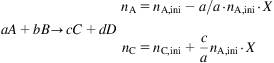
Newton’s Law: Flow in pipes (Newtonian)	Darcy’s Law: Flow through porous media
$\tau =-\mu \frac{dv}{dz}$ (2.65) (2.65)	$v=-\frac{K}{\mu }\frac{dp}{dz}$ (2.66) (2.66)

2.4.1.5 Kinetics and reactor design

Reactors are modeled using differential mass and energy balances. Furthermore, for plug flow or packed bed reactors, pressure drop is another variable. Here we briefly present the equations used to model a batch reactor, such as bioethanol production or packed bed reactors, like the ones in ammonia, methanol, or sulfuric acid production (see chapters: Nitric acid, Sulfuric acid, Biomass). The balances are based on differential mass and energy balances:

$\mathrm{In}\mathrm{flow}+\mathrm{Generation}–\mathrm{Out}\mathrm{flow}=\mathrm{Accumulation}$ (2.67)

(2.67)

2.4.1.5.1 Batch reactors

Mass balance:

$(-r_{\mathrm{A}})=-\frac{1}{V}\frac{d{N}_{\mathrm{A}}}{dt}$ (2.68)

(2.68)

Energy balance:

$\left(N_{\mathrm{Ao}}\left(\sum _{i=1}^n{\mathit{\Theta }}_i{c}_{p,i}+X\mathrm{\Delta }{c}_p\right)\right)\frac{dT}{dt}=UA(T_{\mathrm{a}}-T)+(-r_{\mathrm{A}})\left[\mathrm{\Delta }{H}_{\mathrm{R}}(T_{\mathrm{R}})+\underset{T_{\mathrm{R}}}{\overset{T}{\int }}\mathrm{\Delta }{c}_{p}dT\right]$ (2.69)

(2.69)

2.4.1.5.2 Plug flow/packed bed reactors

Mass balance:

$-\frac{d{F}_{\mathrm{A}}}{dW}=(-r_{\mathrm{A}})$ (2.70)

(2.70)

Energy balance:

$F_{\mathrm{Ao}}\left(\sum _{i=1}^n{\mathit{\Theta }}_i{c}_{p,i}+X\mathrm{\Delta }{c}_p\right)\frac{dT}{dW}=UA(T_{\mathrm{a}}-T)+(-r_{\mathrm{A}})\left[\mathrm{\Delta }{H}_{\mathrm{R}}(T_{\mathrm{R}})+\underset{T_{\mathrm{R}}}{\overset{T}{\int }}\mathrm{\Delta }{c}_{p}dT\right]$ (2.71)

(2.71)

Ergun Equation:

$\frac{dP}{dW}=-\frac{G(1-\varphi )(1+\epsilon X)}{{\rho }_{\mathrm{b}}{A}_{\mathrm{c}}{\rho }_{\mathrm{o}}{g}_{\mathrm{c}}{D}_{\mathrm{p}}{\varphi }^3}\left[\frac{150(1-\varphi )\mu }{D_{\mathrm{p}}}+1.752G\right]\frac{P_{\mathrm{o}}}{P}\frac{T}{T_{\mathrm{o}}}$ (2.72)

(2.72)

2.4.1.6 Design equations for the units

There are a number of books within the chemical engineering field that gather design rules of thumb for a large number of equipment types that help estimate energy consumption, operation of gas–liquid contact equipment, etc, eg Walas (1990).

Putting together the equations results in a large and nonlinear problem that can be solved using state-of-the-art software and solvers such as GAMS, gPROMS, and MATLAB.

2.4.2 Modular Simulation

This is the case for commercial software such as CHEMCAD or ASPEN plus, which have the units modeled as modules. Any time a property (ie, density, enthalpy, etc.) must be computed, a thermodynamic package is called that returns the value. The best performance for this software is the sequential solution of the flowsheet, since the models for each unit are very efficient and connecting them is easy. Dealing with recycling involves tearing of the streams. This technique can be automatic within the software, or can be done iteratively. For instance, for a flowsheet like the one given by Fig. 2.16, we compute stream 2, guess stream 6′, compute 3, 4, 5, and 6, and iterate until 6′=6.

2.5 Optimization and Process Control

Industrial processes must be profitable, and that requires optimization of the use of raw materials and energy. It is not the aim of this book to present the use of optimization for the design of chemical processes since there are a number of works better suited (Biegler et al., 1997). However, it is necessary to familiarize the reader with the existence and current use of mathematical optimization techniques in decision-making as a way to unveil nonobvious trade-offs. Furthermore, process control also deals with feasible operation of processes. Therefore, a process that is unstable or difficult to control is of no use in the chemical industry. We refer the reader to those courses and textbooks that address these issues in detail.

2.6 Safe Process Design

The chemical industry suffers from a number of risks due to the practices and species that are involved (Trenz, 1984). In particular, the main safety problems are related to leaks, either energy or mass leakages, fire, explosion, or uncontrolled chemical reactions. There are two concepts that we must define: hazard and risk. Hazard represents the source of danger. It is what can cause the accident. Risk measures the probability and the consequences of the accident. In other words, the possibility that an accident occurs from a particular danger, and that it causes damages and injuries, as well as impact. Thus we can compute:

$\mathrm{Risk}=\mathrm{Frequency}·\mathrm{consequences}$ (2.73)

(2.73)

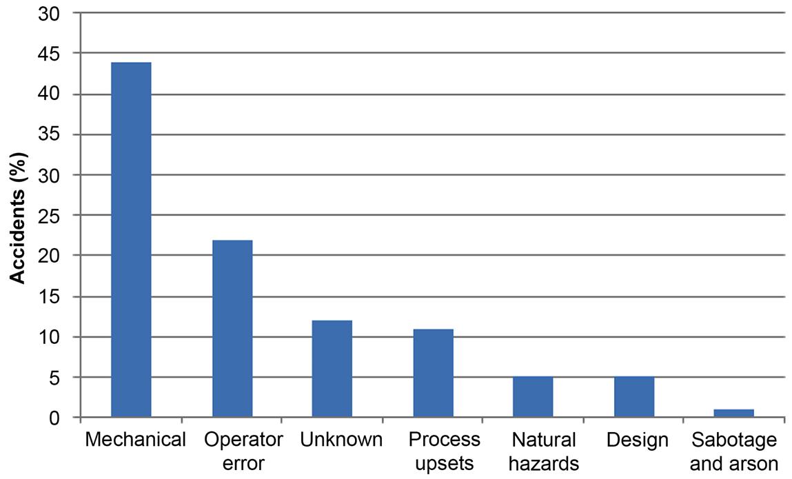
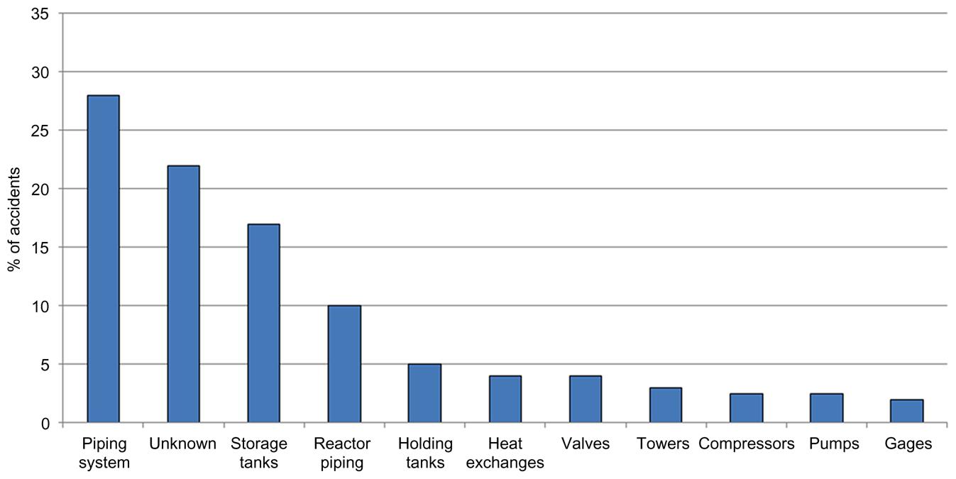
Typically, the main reasons for accidents in the chemical industry are related to mechanical problems in the units; up to 44% of accidents are due to this fact. Twenty-two percent of accidents are because of operator error, while 12% are of unknown cause. The fourth major reason, which accounts for 11% of ocurrences, is due to problems in the process. On the other hand, only 1% is due to sabotage or arson. Fig. 2.17 shows these numbers. The hardware involved in the accidents is, in most of the cases, the piping system (up to 28% of the times). Seventeen percent of accidents are due to storage tanks, 10% due to the piping system of the reactor, and 5% due to holding tanks. In general, the storage of chemicals represents a major danger. Fig. 2.18 shows the main hardware involved in accidents.

With this information at hand, industry has worked hard from different points of view to address safety issues. They can be classified into two approaches (Trenz, 1984).

Traditional approach: When a process is already out there, there is not much that can be done to change it. Mitigation and prevention measures are the most effective techniques.

Current approach: It is called inherently safe design. Safety is another criteria along the decision-making process that leads to the design of a process. The basic idea is to remove the sources of danger. It is based on the talk that Trevor Klentz presented to the Society of Chemical Industry in 1977. In consists of four main pillars:

Based on these principles, we follow a procedure to implement them along with the design of a novel process. Typically, there are three moments along the plant design when we take into account safety considerations in process design decisions, as seen in Fig. 2.19.

2.6.1 Preliminary Hazard Review

The first moment when safety must be included in the decision-making process for process design is during the feasibility study. At this point we should do the following:

List the process alternatives as a function of their safety.

Review the consequences on employees, the public, and the environment.

Review the impact of loss of utilities.

Compute the DOW index of fire and explosion. The DOW index is a quantitative method that provides an objective measure of the actual fire, explosion, and reactivity potential of the equipment and its content. It can help define the areas of potential losses.

$\mathrm{DOW}=\mathrm{Material}\mathrm{factor}·\mathrm{Process}\mathrm{Unit}\mathrm{hazard}\mathrm{factor}$

Material Factor corresponds to the intrinsic rate of potential energy release caused by fire or explosion produced by combustion or chemical reaction.

Process Unit Hazard Factor incorporates all factors that are likely to contribute to the occurrence of fire or explosion incidents. The ranking is given below:

1–60	Light
61–96	Moderade
97–127	Intermediate
128–158	Heavy
≥159	Severe

2.6.3 Detailed Design Review (Basic Engineering)

At this point, the aim is to identify potential problems associated with safety, reliability, and operability (HAZOP). Critical hazards, if identified, shall be quantified to ensure acceptable low risk. Design must be checked against all internal company standards to ensure compliance.

The HAZOP is a structured technique to identify hazards resulting from potential malfunctions in the process. However, it is essentially a qualitative process (see Fig. 2.20). The advantage of using it is that if performed early enough in the design stage, costly modifications after the plant is built can be avoided.

The typical composition of the HAZOP team to carry out the analysis consists of process engineers, chemists, design engineers, instrumentation engineers, production supervisors, and safety and environmental engineers.

Process design has to handle all the possible operating conditions, not only those ideal or typical, including startup, shutdown, process upsets, seasonal changes in the incoming raw materials, and atmospheric conditions. Therefore, it must be tested to validate it at different scales, from plant trials to pilot plant or laboratory scale, so that the design specifications are met. A workplace is a safe place, but it is not only for safety reasons that we must consider safety issues during process design; safe designs save money.

2.7 Process Sustainability

Sustainable development is a production model by which satisfying the needs of current society still maintains the rights of future generations to continue satisfying their needs. Reaching this level of thinking and compromise has been possible due to the current concern for the environment and our legacy to future generations. It represents an equilibrium between the profitable operation of the process, its social acceptance, and its considerations for environmental protection. In this way, three pillars support the entire production scheme. On the one hand, we aim to preserve the nature and environment. Furthermore, economic sustainability aims for an efficient use of raw materials and support for the use of renewable ones. Finally social sustainability aims for dignity and respect for human rights in the market economy context. Therefore, we deal with a multiobjective problem that was to be applied to the entire supply chain, not only to a particular process. Novel metrics have been developed of late to account for these three pillars in the context of process design and the chemical supply chain. While economic evaluations are a widespread practice in the chemical industry, LCA has recently been developed to include environmental effects into the analysis, and models like Jobs and Economic Development Impact (JEDI) account for the effect of the process on the economic growth of the region.

As in the previous case for the safety of a plant, there are two main approaches to deal with the wastes generated in a chemical facility:

2.8 Problems

P2.1. Determine the minimum consumption of hot and cold utilities for the steams in Table P2.1.

P2.2. Determine the minimum consumption of hot and cold utilities for the steams in Table P2.2.

P2.3. A mixture of methanol (Tb=64°C), ethanol (Tb=78°C), propanol (Tb=97°C), and butanol (Tb=117°) with α_Met/Et=2, α_Et/Prop=1.9, and α_Prop/butanol=3.5 is to be separated into pure components. The molar rates (mol/s) are 6, 20, 5, and 4, respectively. Determine the optimal distillation sequence for ethanol as the main product.

P2.4. A five-component mixture, ABCDE, in order of decreasing volatility, is to be separated. The total flow rate is 1 kmol/s, and the composition is as follows (A B C D E)=(0.2 0.4 0.1 0.1 0.2):
Regular distillation,

${\alpha }_{\mathrm{AB}}=2,{\alpha }_{\mathrm{BC}}=1.7,{\alpha }_{\mathrm{CD}}=1.5,{\alpha }_{\mathrm{DE}}=1.04(\mathrm{ABCDE});$

Extractive distillation,

${\alpha }_{\mathrm{AC}}=2.5,{\alpha }_{\mathrm{AB}}=2.4,{\alpha }_{\mathrm{CB}}=2,{\alpha }_{\mathrm{BD}}=2,{\alpha }_{\mathrm{DE}}=1.7(\mathrm{ACBDE}).$

P2.5. A mixture of four species needs to be fractionated. Determine the optimal sequence of columns. Two alternative technologies are available: regular distillation and extractive distillation. The initial flowrate is 1000 mol/h and the composition in molar fraction is as follows: A=0.1; B=0.2; C=0.3; and D=0.4. Additional data for the example:
Regular distillation,

${\alpha }_{\mathrm{AB}}=2,{\alpha }_{\mathrm{BC}}=1.5,{\alpha }_{\mathrm{CD}}=1.02,(\mathrm{ABCD});$

Extractive distillation,

${\alpha }_{\mathrm{AB}}=2.1,{\alpha }_{\mathrm{BC}}=1.5,{\alpha }_{\mathrm{CD}}=1.4(\mathrm{ABCD}).$

P2.6. Determine the minimum approximation temperature among the hot and cold streams so that the cold utility removes 1370 kW and the hot utility provides 390 kW for the streams in Table P2.6.

P2.7. Determine the minimum utilities consumption considering ΔT=10°C for the streams in Table P2.7.

P2.8. Determine the utility requirements for the system represented in Fig. P2.8. The hot composite and the cold composite curves are given as (-) and (--), respectively. Assume ΔT=25 K.

P2.9. Determine ΔT for the system in Fig. P2.9 if the hot utility provides 1000 kW. In the figure (-) represents the hot composite curve, and (..), the cold composite curve.

P2.10. Determine the sequence of distillation columns required to separate a mixture of six components A–F into individual species. The molar flows are 15, 5, 20, 25, 55, and 10 kmol/h, respectively, and the order of volatilities is ABCDEF from higher to lower. The relative volatilities are as follows:

$\begin{array}{l}{\alpha }_{\mathrm{AB}}=1.05,{\alpha }_{\mathrm{BC}}=2.5,{\alpha }_{\mathrm{CD}}=1.85,{\alpha }_{\mathrm{DE}}=1.9,{\alpha }_{\mathrm{EF}}=2.5\hfill \\ {\alpha }_{\text{AB},\text{extractive}}=1.05\hfill \end{array}$

P2.11. Determine the sequence of distillation columns required to separate a mixture of six components A–F into individual species. The molar flows are 40, 5, 10, 25, 30, and 45 kmol/h, respectively. The order of volatilities is ABCDEF from higher to lower. The relative volatilities are as follows:

$\begin{array}{l}{\alpha }_{\mathrm{AB}}=1.05,{\alpha }_{BC}=2.5,{\alpha }_{\mathrm{CD}}=1.05,{\alpha }_{\mathrm{DE}}=1.8,{\alpha }_{\mathrm{EF}}=2.5\hfill \\ {\alpha }_{\text{AB},\mathrm{extractive}}=1.7,{\alpha }_{\text{CD},\mathrm{extractive}}=1.8\hfill \end{array}$

P2.12. Compute the minimum requirement of utilities and design the optimal network among a set of cold (C) and hot (H) streams in Table P2.12.