
Learning by Classification and Discovery
This chapter will explain methods for learning by classification and discovery. The first half of this chapter describes a classification method using decision trees and Bayesian statistics. A decision tree can be generated by a simple algorithm and is an efficient method of finding regularities of massive data. Bayesian statistics can be applied to a learning algorithm for data that include noise.
The second half of this chapter explains learning by discovery as a method for problems with unknown goals. Learning by discovery can be formalized as the problem of generating new representations from data and knowledge.
9.1 Representing Instances by a Decision Tree
Let us consider the classification of objects into classes that are defined by a set of attribute-value pairs. This can be done by generating a decision tree where each class corresponds to a leaf and the classes are discriminated by tests at intermediate nodes. In order to explain how to learn to classify objects by generating a decision tree, first let us consider a method of representing objects using a decision tree.
We assume that a positive instance of a concept is represented by a set of attribute-value pairs. For example, if we want to represent “it is fair weather, low temperature, low humidity, and no wind” as a positive instance of the concept “weather,” we can use
| instance name | attribute | value |
| instance1 | weather | fair |
| temperature | low | |
| humidity | low | |
| wind | no |
When such instances are given as data, we can represent the data as a tree structure. Below we call instances data.
For example, the set of data shown in Figure 9.1(a) can be represented as the tree shown in Figure 9.1(b). In this tree, an intermediate node of the tree corresponds to the test of whether an attribute is included in the data or not, and an edge corresponds to a value. Each leaf of the tree represents some particular subset of data. Nodes and edges that correspond to attribute-value pairs not included in the data are omitted in Figure 9.1(b).
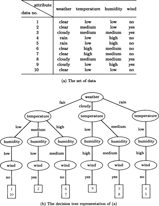
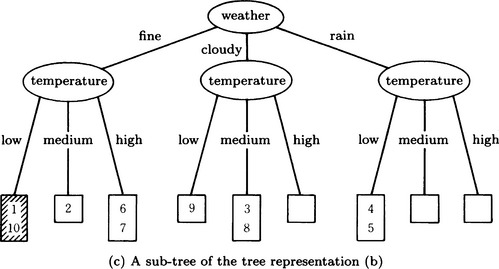
A substructure of the data represented by a tree like Figure 9.1(b) can be represented by an appropriate subtree. For example, Figure 9.1(c) is a subtree of the tree shown in Figure 9.1(b). The leaves of this subtree correspond to a subset of the given set of data. The leaf shown with the oblique line in Figure 9.1(c) corresponds to the set of data that satisfy the condition “it is fair weather and low temperature,” in other words, the set of data 1 and 10. In this way, we can concisely represent the characteristics of massive data using subtrees.
The tree representation of a concept as shown above is generally called a representation by a decision tree.
On one hand, a decision tree is one of the methods for representing a set of data declaratively. On the other hand, if we regard the procedure for following a path from the root of the tree to a leaf as representing the leaf, a decision tree can be thought of as a procedural representation of a set of data. For example, Figure 9.2 is the procedural form of the decision tree representation in Figure 9.1(c). However, note that, in this representation, the order of testing attributes is from the root of the decision tree to the leaves and is determined beforehand.
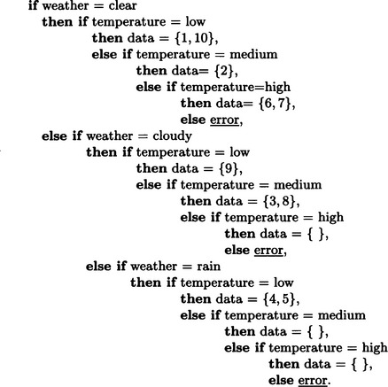
Figure 9.2 A procedural representation of the decision tree shown in Figure 9.1(c)
One advantage of considering a decision tree as a procedural representation is that we can easily represent a procedure for adding new data to the decision tree. When a procedure like Figure 9.2 is given, all we need to do to add new data, d, is to apply the procedure to d, and when d is found to be classified into leaf D, update D to D = D U {d}. Also, we can test by checking if d ∈ D whether d is new data and whether it matches already given data. A decision tree is useful both as a representation of massive data and as a procedure for adding new data.
9.2 An Algorithm for Generating a Decision Tree
In order to classify a set of data that is defined by a set of attribute-value pairs into several mutually exclusive clusters, it is sufficient to generate a decision tree representation for the data in which each leaf corresponds to some cluster. In this section we will explain a method for doing this.
As an example, let us consider the 16 objects shown in Table 9.1. This data is the information on 16 cars and consists of four attributes—the amount of exhaust, the type, existence of automatic transmission, and the color—and their corresponding values. Also, in Table 9.1, each object is classified into one of the two classes, positive instances (P) or negative instances (N). To classify the data into P or N, we can use, for example, the well-formed formula
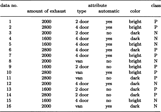
and label the data with value T by P and the other data by N. Here we represent the data as a decision tree.
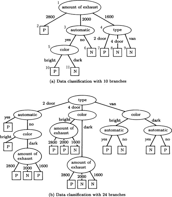
The decision tree in Figure 9.3(a) is equivalent to the representation in (9.1) in the sense that all data can be divided into P or N. The number of branches at each node in this tree is three for the amount of exhaust and the type, two for automatic transmission, and two for the color, 10 in total. Also, the decision tree in Figure 9.3(b) describes the same classification as (9.1). However, the number of branches in this tree is 24. There are generally many decision trees that classify the same set of data into clusters. This suggests that we need to generate a decision tree that can classify data efficiently.
Generally, the efficiency of a decision tree for classification depends on how simple the tree structure is. The simplicity of the tree structure can be evaluated by applying information theory. Below, we describe an algorithm for generating a decision tree for efficient data classification based on elementary information theory.
Suppose we are given a finite set of data D. Furthermore, suppose that there is a finite number of tests common to all data, t1,…,tn, and that the value viP for each attribute p ∈ {q1,…, qi} is obtained by giving the test ti to the data d. For example, for the data in Table 9.1, we set ti to be the function that gives the value Vip to the ith attribute. As an example, taking data1 and the amount of exhaust as t1, we get v11 = 2000. If we define v = f(d, t), using a function f to make the data d and the test t correspond to v, then in this example, 2000 = f(data1, amount of exhaust).
Suppose a finite number of classes c1,…, cm are given and each datum d falls into one of the c1,…, cm. For example, for the data in Table 9.1, there are two classes, P and N, and the data1 falls into P. Here, we can define c = g(d), using a function g that makes a class correspond to the data. For instance, P = g(data1) in the above example. For the set D of these data, let us consider an algorithm for generating a decision tree.
First we consider a list of three items: the node number, an edge from this node, and the node number of the child node connected by the edge. We represent a decision tree using a set of these lists. For example, the decision tree in Figure 9.3(a) can be represented as

Since using node numbers makes things complicated, we will use a test at a node instead of its node number. For example, in the decision tree in Figure 9.3(a), we will use the list (amount of exhaust 2800 P) instead of (1 2800 2). This sometimes creates two identical lists in a decision tree, but here we assume that there is only one instance of a list in a decision tree. When two identical lists exist, we can argue similarly by attaching different numbers to them. For the data in Table 9.1, the set of tests is
The set of values for each test is
Also, we represent the set of data D by a set of data numbers. For the data in Table 9.1 we use
When a leaf corresponds to a test in a decision tree, such a leaf is called an active node. The trees in Figure 9.3(a) and (b) do not have active nodes. A path from the root of a decision tree, s0, to a node s is represented as the list of nodes, Q(s) = (s0,…, s), where we use tests, or the values of tests, instead of node numbers. Consider the following algorithm:
Algorithm 9.1
(generating a decision tree for data classification)
[1] If D = ∅, then stop. H = ∅ is the decision tree we want.
[2] If c = g(dk) for all dk ∈ D, in other words, if all dk ∈ D are classified into the same class, set H = {(nil nil c)} and stop. H is the decision tree we want. Here {(nil nil c)} means the tree with only the root node c.
[3] Choose a test ti ∈ {t1,…,tn} and set H = {(nil nil ti)}. (By definition, t1 becomes an active node.)
[4] If an active node does not exist in H, stop. H is the decision tree we want.
[5] Choose one active node in H, and let it be si. Let Dij (j = 1,…, qi) be the set of dk ∈ D(Si) such that vij = f(dk, si), where D(si) is the subset of D in which the values of the tests corresponding to elements of Q(Si) − {Si} are fixed. For each Dij, do (1) and (2):
When (1) and (2) have been executed for all dij, go to [4].
As an example, let us generate using Algorithm 9.1 the decision tree in Figure 9.3(a) from the data in Table 9.1.
Since conditions [1] and [2] of Algorithm 9.1 do not hold, go to [3].
[3] Choose the test “amount of exhaust.” Set H = {(nil nil amount of exhaust)}.
[4] Since the conditions are not satisfied, go to [5].
[5] If we choose “amount of exhaust” as the active node of H, then D(amount of exhaust) = D. So, consider the following three cases:
For (i), g(d) = P for all d. Therefore, set H = {(nil nil amount of exhaust), (amount of exhaust 2800 P)}. Next, for (ii), all d′s cannot be classified into one class. So, choose a new test from {amount of exhaust, type, automatic, color} – {amount of exhaust}, where Q(amount of exhaust) = {amount of exhaust} was used. Now choose “automatic” as the test and set
For (iii), as in (ii), choose a new test from {amount of exhaust, type, automatic, color} – {amount of exhaust}. Suppose we pick “type” here. In this case, we have
[4] Since the conditions are not satisfied, go to [5].
[5] The active nodes of H are “automatic” and “type.” If we choose “automatic,” D(automatic) = {1,3,7,8,12,16}. So, consider the following two cases:
(i) for d = 1,7,12,16 yes = f(d, automatic)
(ii) for d = 3,8 no = f(d, automatic)
For (i), choose a new test from {amount of exhaust, type, automatic, color} – {amount of exhaust, automatic}. Now, suppose we choose “color.” We set H = H U {(automatic yes color)}. For (ii), since g(d) = N (d = 3,8), set H = H U {(automatic no N)}.
[4] Since the conditions are not satisfied, go to [5].
[5] Suppose we choose “type” from active nodes of H. Then D(type) = {4,5,9,13,15}. Consider the following:
(i) d = 9,13 two_door = f(d, type)
(ii) d = 4,5,15 four_door = f(d, type)
In (i), since g(d) = P, set H = H U {(type two_door P)}. In case (ii), since g(d) = N, set H = H U {(type two_door P)}. Also, since a d that makes f(d, type) = van does not exist, define g(0) = N and set H = H U {(type van N)}.
[4] Since the conditions are not satisfied, go to [5].
[5] For the active node of H “color,” update H = H U {(color bright P) (color dark N)} using the same method as described above.
The H at the end is the decision tree in Figure 9.3(a) itself. If we use the decision tree generated by Algorithm 9.1, we can classify new data. For example, if we want to classify the following new data:
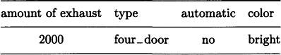
using the decision tree in Figure 9.3(a), we find that these data can be classified as N. Also, if this classification is a mistake and the data should be classified as P, rewrite (automatic new N) in the decision tree H to (automatic new type) or (automatic no color) and reexecute [5]. By doing this, we can expand H and classify data correctly. The expansion of a decision tree is generally done using the following algorithm.
Algorithm 9.2
(adding new data to a decision tree)
[1’] If the decision tree H already exists and new data d whose class is known is given, go to [6].
[6] If the class c that is obtained by letting d go though H matches the correct class of d, then stop. Otherwise, choose a new test ti ∈{t1,…,tn} − Q(c). Also, let (t v c) be the last edge in the path Q(c). In this case, set H = H U {(t v ti)} − {(t v c)} and go to [5] in Algorithm 9.1.
9.3 Selecting a Test in Generating a Decision Tree
In the algorithm for generating a decision tree that was described in Section 9.2, what to choose as a new test changes the complexity of the decision tree. This is easily seen if we compare (a) and (b) in Figure 9.3. Below, we will describe a method for generating the simplest (by one measure) decision tree possible.
Suppose the data in a data set D are classified into different classes c1,…, Cm by the decision tree H. Also, suppose that the number of data that fall into Ci is di. We assume that the probability of new data being classified into ci is ![]() In other words, we regard the size of the data subset to be classified to be the same as the probability. Under this assumption, we can look at H as a stochastic information-processing machine. In other words, H can be considered to be a machine for transmitting a message ci with probability
In other words, we regard the size of the data subset to be classified to be the same as the probability. Under this assumption, we can look at H as a stochastic information-processing machine. In other words, H can be considered to be a machine for transmitting a message ci with probability ![]() In this case, the amount of information that the machine H transmits is given by
In this case, the amount of information that the machine H transmits is given by
Now suppose, for the same decision tree H, the root node corresponds to the test tj and tj may take nj different values Vj1,…, vjnj. We set Djk = {d ∈ D/f(d, tj) = vjk} (k = 1,…,nj) for these values. Furthermore, suppose each Djk includes ![]() items of data that fall into the class Ci. The partial tree Hjk that corresponds to Djk can be considered to be a stochastic machine where the amount of information is given by
items of data that fall into the class Ci. The partial tree Hjk that corresponds to Djk can be considered to be a stochastic machine where the amount of information is given by ![]() , as in (9.2). Therefore, the amount of information is
, as in (9.2). Therefore, the amount of information is
Of (9.2) and (9.3), (9.2) is the amount of information for the decision tree H; (9.3) is the amount of information for the decision tree when we choose a test tj for the root node of H. Therefore, the increase in the amount of information as a result of choosing tj is
So, as a method for choosing a test when generating a decision tree, we can use a method that chooses tj so that
This method can be applied not only to the root node but also to any node in the decision tree. Since E(d1,…, dm) is a constant independent of the choice of the test, from (9.4), maximizing G(tj) and minimizing E′(tj) yield the same value.
We will now explain a method for choosing a test by maximizing G(tj) using the data in Table 9.1. We will only show what to choose as the test for the root node; however, we can repeat this method for the intermediate nodes. First, nine data are in the class P and seven data are in the class N, so if we set d1 = 9, d2 = 7, we have
Next, we compute G(tj) as follows for the four tests “amount of exhaust,” “type,” “automatic,” “color.”
From these, we can obtain the maximum of G(tj) for t1 = “amount of exhaust.” So, in generating the decision tree, if we choose “amount of exhaust” as the test at the root node, we can increase the amount of information at the root node to a maximum, as in the decision tree in Figure 9.3(a). As opposed to this, the tree in Figure 9.3(b) chooses as the test at the root node, “type,” which results in only a small increase in the amount of information.
In the method above, when choosing a test at each node, we need to check the classes of all the data for each possible test. Therefore, the computational complexity of the above procedure is on the order of O(x y. z) where x is the amount of data, y is the maximum number of possible tests, and z is the number of times we choose a test. This is not an exponential function of x, so it is possible to classify massive data efficiently.
9.4 Learning from Noisy Data
As we described in Section 9.3, in learning by generating a decision tree, the amount of computation necessary to generate a decision tree depends a lot on which test is chosen at each node. This becomes a serious problem particularly when there is noisy data, and data can be classified into wrong classes. Not only when using decision trees but also in dealing with massive data in general, learning from noisy data is an important problem. In this section we treat learning from noisy data.
(a) Generating a decision tree from noisy data
First, let us describe briefly learning by generating a decision tree with data containing noise. We look at whether the amount of information in the decision tree increases significantly when choosing a test tj at a node. In order to do this, let us consider the probability that the value of tj is independent of the class distribution d1,…, dm of the data set D:
Also we consider the χ2 distribution of degree of freedom nj − 1
If the value of ![]() (i = 1,…, m) is not small, we can test the hypothesis “tj is independent of the class distribution of D” using expression (9.5). In other words, if we do the x2-test at the 1% condidence level and the hypothesis is not rejected, we should not choose tj as a test. However, in the case that no tj is chosen, another method that chooses the class Ch giving dh = max{d1,…, dm} instead of a test is also possible.
(i = 1,…, m) is not small, we can test the hypothesis “tj is independent of the class distribution of D” using expression (9.5). In other words, if we do the x2-test at the 1% condidence level and the hypothesis is not rejected, we should not choose tj as a test. However, in the case that no tj is chosen, another method that chooses the class Ch giving dh = max{d1,…, dm} instead of a test is also possible.
We can generate a decision tree efficiently to some extent even if the data include noise. The above method is effective when all the data are presented simultaneously. It is difficult to apply this method when the data are presented incrementally.
(b) Processing errors in incrementally presented data
Let us consider a learning method when data are presented incrementally and include noise (in other words, the data are classified erroneously). First, we will discuss a method of processing errors for data presented incrementally based on Bayes’ theorem.
Suppose we classify data obtained by observations and experiments into several classes. To simplify, we suppose there are two classes, 0 and 1. Possible errors occur when the data that are supposed to be classified into 0 are classified into 1 and when the data that are supposed to be classified into 1 are classified into 0.*
To avoid these errors, let us represent a class statistically as one point on the interval [0,1]. For example, we allow a classification such that the (stochastic) class for the data “is 0.2.” In this case, if the true class of the data is 0, the error rate is 0.2; if the true class is 1, the error rate is 0.8. Furthermore, suppose we have a set of data D consisting of d0 items in class 0 and d1 items in class 0. The (stochastic) class that minimizes the square sum of the error rate for the classification of each datum in D is given by d1/(d0 + d1). (There is another method where, for the set D, if d0 > d1, then the class is 0, and if d0 ≤ d1, then the class is 1. These classes minimize the sum of the rate of errors in the classification of the data.)
This method is the same as the one described in Section 9.3. The method is simple, but effective when massive amounts of data are presented simultaneously. However, in actual observations and experiments, data are usually presented incrementally rather than simultaneously. In this case, we can use Bayes’ theorem as a method for dealing with errors in classification.
Let us suppose we need to judge whether a given datum is a positive instance of a concept c or not when c is represented as a set of attribute-value pairs. If we let x be the stochastic event that the datum is a positive instance of c, and let a be the event that A is an attribute of c, we can define the ratio that the expected value of the probability that x occurs is enhanced by A as
where ![]() is a complementary event of a stochastic event, e.
is a complementary event of a stochastic event, e.
On the other hand, the ratio that the expected value of the probability that x occurs is reduced by A can be defined as
Now, if we can compute s1 and s2 for all attributes A of c, their product represents a measure for judging whether the datum is a positive instance of c or not. In other words, the bigger the value of the product, the bigger the chance of being a positive instance. Actually, we cannot compute s1(a, x), s2(a, x) directly using the above definition. However, there is a simple approximation method described below.
First, note there are four kinds of matching of a datum and an attribute:
Of these, (1-2) and (2-1) are the cases that cause error. (1-2) causes errors of the first kind and (2-1) causes errors of the second kind.
Now let us consider matching a datum to a concept, and let mp, up, mn, un be the number of items for (1-1), (1-2), (2-1), (2-2), respectively. Then, s1(a, x) and s2(a, x) that are defined by (9.6) and (9.7) can be approximated by
Let us prove this.
First, from Bayes’ theorem, ![]() for any stochastic events e1 and e2. This can be applied to (9.6) and (9.7) as follows:
for any stochastic events e1 and e2. This can be applied to (9.6) and (9.7) as follows:
On the other hand, if we set N = mp + up + mn + un, by the definitions of mp, up, mn, un we have
Also, if we use ![]() we have
we have
By substituting (9.10), (9.11) into (9.9), we obtain the expressions (9.8).
Since mp, up, mn, un can be incremented each time a new datum is provided, the expressions in (9.8) can be recomputed easily each time a new datum is given.
Now, as a parameter for checking whether the concept c itself is a concept for some “positive instance” or not, we introduce
The computation of cp can be done easily each time a new datum is given.
If we use (9.8) and (9.12), the parameter for checking whether the datum x is a positive instance of the concept c or not can be given by
Also, from what we explained above, xp can be recomputed each time a new datum is given.
(c) Learning by incremental presentation of noisy data
We will explain a method for learning to classify data when noisy data are given incrementally. First, let us consider a method for judging whether the datum x presented incrementally is a positive instance of a concept c or not, when c is represented as a set of attribute-value pairs. Such a method needs at least the following functions:
Below, we consider a method of learning using the functions (1)-(4). First, let us look at (1). Suppose we are given the attributes A1,…, An and the values that Ai can take are ai1,…,aiki. Then we define the representation of a concept as follows:
(i) We represent as αij a possible value that the attribute Ai can take. Then, a characterization generally means the predicate Ai(αij), its logical conjunction, or disjunction.
(ii) A concept description element is a triple consisting of a characterization and two parameters, wp and wn, where wp and wn each are weight parameters whose value becomes larger as the characterization of positive and negative instances becomes better.
(iii) A concept is a finite set of conceptual description elements.
For example, suppose the attributes of various liquids and their possible values are given. Then, temperature(hot), temperature (hot)∨viscosity (low), color (orange) ∨ color (red), temperature (warm) ∧ color (orange) ∨ color (red) ∨ viscosity (medium) are characterizations. Since the set of an attribute’s possible values is given beforehand, the negation of an attribute’s value can be represented using a disjunction. For example, a description of the characteristic “viscosity is not high” can be represented as
Therefore, all well-formed formulas using ∧ ∨, ∼ for a given value of an attribute can be represented using definition (iii).
When the representation of a concept is defined like this, we need to give the initial representation of the concept at the beginning in order to be able to judge whether an incrementally presented datum is a positive instance of the concept or not. For example, let us choose the following as the initial representation. First, consider the concept description element (Ai(aij), 1,1) where wp = 1, wn = 1, and Ai(αij), the predicate representation of any attribute-value pair that does not include a conjunction or disjunction, is a characterization. Then, we let the set consisting of all of those elements, {(Ai(aij), 1, 1)|(j = 1, …,k;i = 1,…, n)}, be the initial representation. For example, the initial representation for the attribute-value pairs in Figure 9.4(a) can be given by Figure 9.4(b).

Now, let us assume we have the initial representation of a concept. Then, suppose we are presented with the first datum x. What we will do is (2), in other words, match the concept with the datum. This can be done by the method described in (b) by obtaining cp, mp, up, mn, un in the following way:
Algorithm 9.3
(matching a concept with a datum)
[1] Check whether the attribute of the datum d matches with each concept description element that makes up the concept.
[2] If they match, increase by 1 the value of wp that corresponds to this attribute. If not, increase by 1 the value of wn.
[3] In addition, find cp, mp, up, mn, un from the result of matching for each description element, and compute the value of the parameter xp suggesting that x is a positive instance from cp, mp, up, mn, un using (9.13).
Since the datum x has the possibility of including noise, this method does not always correctly determine whether a datum is a positive instance or not. What it can do is to determine the probability of being a positive instance. It is important for this kind of stochastic method to have an evaluation function that judges whether the representation of the concept is appropriate or not. This function is in (3). (3) is computed by updating the values of weight parameters as in [2] of Algorithm 9.3.
Finally let us look at (4), the correction of a concept. In (4), not only are the weight parameters updated but also the representation for the concept itself is corrected. This is done by searching the the concept representation space. This space is not only finite but has the structure of a complete lattice. Using this structure, we can do generalization, specialization, and negation of a concept.
For example, Figure 9.5 shows a part of the concept representation consisting of the attributes and their values shown in Figure 9.4(a). In this graph, we do specialization by searching upward, i.e., by finding, for instance, a higher node for viscosity (high) and color (white), which is viscosity (high) ∧ color (white). Generalization, on the other hand, searches the graph downward.
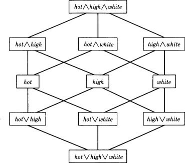
Figure 9.5 Part of the concept representation space defined by the data shown in Figure 9.4(a). (Predicate names are omitted.)
Search of the concept representation space depends on how the current concept representation and the datum are matched. For example, if the datum is misjudged, deciding that a negative instance is a positive instance, we can do specialization because the representation of the current concept is considered too general. Conversely, if the datum is misjudged to be a negative instance when it is actually a positive instance, we can do generalization since the representation is too specific. In either case we can try the negation of the well-formed formula. We can improve the efficiency of the search not only by choosing a generalization, specialization, or negation but also by combining them with various methods of heuristic search.
(d) A learning example
We explain an example of learning based on the above method. Let us consider the case where the data on cars shown in Table 1 are incrementally presented from the top. In this example, the attributes and their possible values for the data are
If we match the data with numbers 1-7 in Table 9.1 with an initial representation similar to the one in Figure 9.4(b), we obtain the result shown in Figure 9.6(a). Here the initial value of mp, up, mn, un is set to 10, and each time the value is changed, we take 99% of the changed value as the new value. For example, in Figure 9.6, the value of mp = 11.77 for the amount of exhaust (2000) means that, of the data that have been input so far, the number of positive instances where the value of “amount of exhaust” is “2000” is 11.77 using the conversion method above.
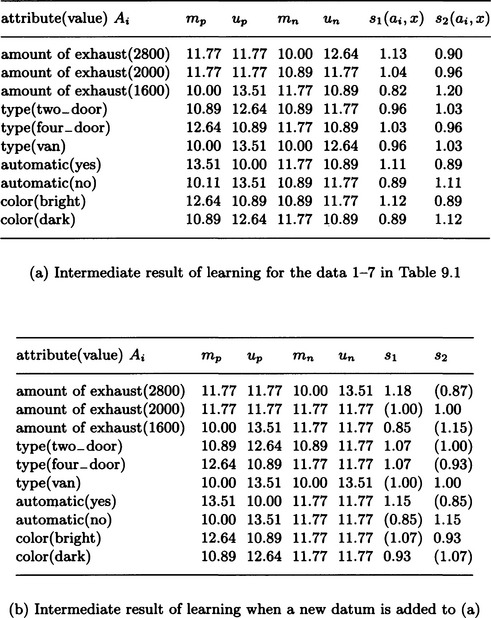
Figure 9.6 Learning example with data presented incrementally. (The data are shown in Table 9.1.)
Suppose we are given a new datum, d: amount of exhaust(2000) ∧ type(van) ∧ automatic(no) ∧ color(bright) (data number 8 in Table 9.1). For each attribute Ai, if we compute s1(ai, d) and s2(ai, d) based on (9.8), we get Figure 9.6(b). By (9.12), the value of the parameter cp becomes cp = 1.00 and, using (9.13) on these values, the probability of d being a positive instance is suggested by xp = 0.77. (The values of s1 and s2 used to obtain xp are in ( ) in Figure 9.6(b).)
As shown in Table 9.1, the datum d is a negative instance. In this case, first we need to update the values of mn and un for each characterization. For example, since the characterization of the amount of exhaust(2000) matches d, we need to increase the value of mn for the amount of exhaust(2000) using the above method. Since the amount of exhaust (1600) does not match d, the value of un is increased to account for the amount of exhaust(1600). Next, we correct the concept representation itself to a more specific one. For example, we find an a that makes s1(a, x) the minimum among characterizations that do not match the negative instance d and find an a′ that makes s2(a’, x) the minimum among the characterizations that match d. We then insert their conjunction explicitly into the representation of c. By this method, in this example, we add amount of exhaust(1600) ∧ automatic (yes) to the original representation. The attribute-value pair where s1 (a, x) takes the minimum value is automatic(no), and “automatic” takes only two values, “yes” and “no.” Thus we can also add the negation, in other words, automatic (yes). In this example, since we can add automatic (yes) by the specialization previously stated, we can also use the heuristic of not adding automatic(yes) but removing automatic (no).
9.5 Learning by Discovery
In most of the learning algorithms we described so far, the goal of the learning is given beforehand. Let’s now look at learning algorithms when the goal is not decided beforehand. Such learning is called learning by discovery. As we will explain below, learning by discovery can be used for finding regularity in massive amounts of data or generating new representations based on knowledge.
(a) Discovering regularities in data and attributes
In this section we provide an algorithm for finding relations among numeric data and representing these relations as variables. This problem, as we describe later, can be formulated as a problem whose goal state is not known beforehand. Its learning algorithm can be represented as an algorithm of search in problem solving. We start by defining a data-vector space and operations on data-vectors as follows:
Definition 1
(data-vector space) Suppose the values of n data xi (i = 1,…, n) for each of the given attributes a1,…, ak are given by vi1,…, vik (i = 1,…, n). Then the n-dimensional Euclidean space including the set of the n-dimensional vectors V = {(v1j,…,vnj)/j = 1,…,k} is called the (n-dimensional) data-vector space.
Definition 2
(product and quotient) We define the producto
and the quotient /
as binary operations on the n-dimensional data-vector space M. Note that only the vectors y that make yi ≠ 0 (i = 1,…, n) are defined.
Let X0 = {x1,…, xn}, a set of data-vectors with more than two elements, and for two arbitrary elements of X0, xi, xj, let X1 = {x1,…, xn, xi oxj} and X2 = x1,…, xn, xi/xj}. Repeating this operation for each of X1 and X2, we can generate an infinite list of sets, X0, X1, X2, …. Here we assume that in a quotient vector xi/xj all the elements of xj are not 0. Let us call this condition (*).
Let us consider X = {X0, X1, X2,…} as the state space, X0 as the initial state, each operation generating X1, X2,… as an operator, and the condition (*) in generating the quotient vector (*) as a constraint on operator application. Then finding a goal state Xg ∈ X can be regarded as problem solving. In particular, when Xg is not given beforehand, finding the goal state becomes learning by discovery according to the above definition.
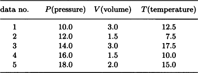
As an example, suppose we have data for the pressure P, volume V, and temperature T for some gas as shown in Table 9.2 (we ignore the units). The problem is to find some regularity among the attributes P, V, and T. Suppose the initial state of the problem is the set of the data-vectors X0 = {p, v, t} where
Then, if we generate new states by repeatedly applying the above operations to the elements of X0, p, v, t, and obtain some interesting state, we can say that we discovered a relation among P, V, T.
If we use breadth-first search on this state space, the states shown in Figure 9.7 are generated. In this case the vector p o v/t becomes a vector whose elements all have the same value (called a constant vector). A state including a vector whose elements have a constant value is an “interesting” state. Actually, the fact that pov/t is a constant vector means that PV/T = constant; in other words, Boyle’s law holds for the data in Table 9.2.
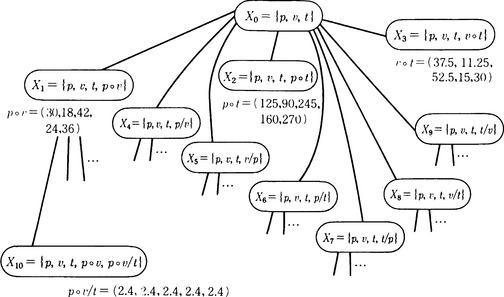
Figure 9.7 Part of the state space generated by breadth-first search from the data of Table 9.2.
This algorithm is very simple, but it can be used to give a new name to a regularity that is found and to discover higher-order regularities by regarding this regularity as a new attribute. For example, suppose we get the data 1-9 as shown in Table 9.3 by measuring the weight of the components in some samples of three kinds of gas consisting of oxygen O and nitrogen N. Suppose we apply the above method for each of the three subsets of data 1-3, 4-6, and 7-9 and, as a result, we obtain the following for the weight wo for oxygen and the weight wN for nitrogen:
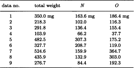
Then, if we define α = wO/wN as a new attribute common to the three kinds of gas, each gas can be said to have the characteristic that the values of the variable a differ by a multiple of an integer.
(b) A search method for discovering regularity
In this section we explain a method for discovering regularity in numeric data that is slightly different from the one explained in (a).
Suppose data are represented as the set of the pairs of attributes a1,…, ak and their values. A data-vector is defined as the vector of those k values for a datum. For such data, let us define the binary operations o (product) and / (quotient) on the data-vector space. We define the graph G which has a1,…, ak as nodes and whose edges are joined only between the attributes when the data-vector becomes a constant vector by the operation of o or /. This graph is called a proportionality graph, and we can consider the following search algorithm for G.
Algorithm 9.4
(proportionality graph search for discovering regularities)
[2] Of the maximal cliques for the graph G, find the maximum clique. Let N be the set of nodes in this clique.
[3] Pay attention only to attributes that correspond to the nodes of N and find a pair of attributes where a constant data-vector is generated by the operation o or /. (For example, use depth-first search.) In this case, generate a new node ai o aj or ai/aj corresponding to o or / and add this node to N. Also, delete ai and aj from N. Set M = MU {ai o aj} or M = MU {ai/aj}. If a pair of such attributes does not exist, then stop. The new nodes that were found so far provide the regularity in the original data.
[4] For the updated set of nodes, N, define edges only for pairs of attributes where a constant data-vector is generated using o or /. Call the resulting graph G and go to [2].
As an example, let us consider a sphere that falls down freely in a viscous medium. Suppose given data have as attributes the mass of the sphere m, the radius r, the density p, the viscosity coefficient of the medium n, the wavelength of the color λ, and the velocity v. If the data do not include noise, the initial proportionality graph G in the above algorithm is the top graph in Figure 9.8. There are three maximal cliques for this graph, {p, r}, {m, r, v, n}, {n, λ}, describing them as sets of nodes. Let us pick {m, r, v, n}, which has the largest number of nodes. If we check the regularity of the data-vectors that correspond to the attributes m, r, v, n, and notice that the vector r/m becomes a constant vector, we obtain the second graph in Figure 9.8. By repeating this process, we finally reach N = {vrn/m}, and the algorithm stops. We have found the regularity that vrn/m = constant for the original set of data.
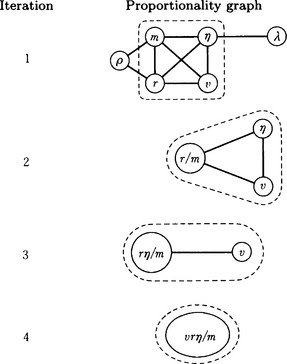
Figure 9.8 The proportionality graph search for a relation among attributes. (The maximum clique obtained during each iteration is shown inside each broken box.)
The discovered characteristic is equivalent to Stokes’ law of the viscosity of a liquid as applied to an object that falls freely.
Since Algorithm 9.4 for the proportionality graph search method chooses only the maximum cliques in [2], it sometimes cannot find regularities that can be found from other maximal cliques. This can be avoided by extending Algorithm 9.4 and doing [3] and [4] for all the maximal cliques. For example, in the example of Figure 9.8, we can obtain the regularity m/pr = constant if we choose {m, p, r} instead of {m, r, v, n} as the node set for the maximal clique.
On the other hand, this search method can cause computational explosion because it may generate and accumulate too many new nodes during the search. One method of solving this problem is the suspension search method. In this method, when the data at a generated node are not constant within predetermined intervals, no further search involving this node is performed. Such a node is called a suspended node. By doing the proportionality graph search only for nodes that are not suspended, we may avoid decreases in the search efficiency to some extent.
(c) Qualitative discovery and processing noise
So far we have described methods for discovering regularities in numeric data. There are also methods for discovering qualitative regularity of data. By classifying given numeric data into clusters, the set of data can be described by a set of rules, not just one rule. In this case, since each cluster can be thought of as a concept that is newly generated from the data, we can use for clustering the method of concept clustering described in Section 6.5. A method for finding regularities for this notion of concept is one example of qualitative discovery. Also, in this section we did not describe methods for processing noise. One method for processing noise is to allow an error range of some extent (for example, 1%) when we check the relation o or / among data-vectors.
9.6 Discovery of New Concepts and Rules
(a) Heuristic knowledge
No totally new and interesting concepts or rules have been discovered by applying the algorithm for discovering regularities described in Section 9.5. Three reasons can be given for this:
(1) Actual data include complicated noise, but the current discovery algorithms do not have powerful methods for dealing with noise.
(2) The amount of data is not sufficient or important attributes are missing.
The most important reason is (3). Knowledge used for discovery is necessary not only for processing data but also for asking what data are missing and for removing noise.
One characteristic of discovery as problem solving is the fact that the goal is unknown. This suggests that the control of search requires a lot of specific knowledge, that is, heuristic knowledge. Having lots of heuristic knowledge is a necessary condition for discovering a new interesting concept or rule. In this section, we will describe an algorithm for discovery based on massive heuristic knowledge and a simple control mechanism.
(b) Discovering a concept based on knowledge
To discover a new concept based on massive heuristic knowledge, we first need to consider how to represent heuristic knowledge. To do that, we use a representation combining frames and rules.
As an example, let us consider the domain of simple arithmetic. The frame representation of a concept in arithmetic can be described, for example, as in Figure 9.9. A slot and its filler, as shown in this example, correspond to an attribute and its value. Some attributes have a value that is fixed at the time the frame is made; other attributes have values that can change.
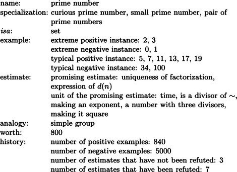
Figure 9.9 A frame representation of “prime number” (modified from Lenat, 1977).
The following is an example of heuristic rules:
if f is a function that transforms an element of the object A into an element of the object B
then consider only the elements of A that are transformed into extreme elements of B.
For example, if A and B are sets of natural numbers and f is a function for “is a divisor of ∼,” we try to generate as subsets of A “a set of numbers without divisors,” “a set of numbers that has only one divisor,” “a set of numbers that has two divisors,” “a set of numbers that has three divisors,” etc. Among them, “a set of numbers that has two divisors” is equivalent to “prime number.”
Suppose we have the following heuristic rule:
If we apply this rule to the function “is a divisor of ∼,” the inverse function of “is a divisor of ∼,” in other words, “multiplication,” is considered. Then, if we apply other heuristic rules for “multiplication,” we can obtain simpler functions.
As we can see, if we repeat the application of heuristic rules starting with known concepts, we might be able to find a new concept. For example, we may generate a concept such as “prime number” and “number with a maximal number of divisors”* from the concept “addition” and “direct product (of sets).”
The application of heuristic rules, as described in Section 9.5, uses frames for concepts and does search “where the goal state is not given beforehand” using best-first search. The direction of the search is determined by the value of the “worth” parameter that appears in each frame and heuristic rules for controlling search that have been set up separately. As the search proceeds, a new frame is generated based on the heuristic rules.
Now, many of the discovery algorithms that we have considered so far use search using heuristic rules. However, if the set of heuristic rules remains fixed, possibly only uninteresting concepts may be generated as new concepts by the search. In this case, a method for discovering heuristic rules enables us to find more interesting concepts using newly discovered rules.
As a method for discovering a heuristic rule itself, heuristic rules can be thought of as concepts and the methods described above can be used. Heuristic rules can be represented as a frame just as was done for concepts, and heuristic knowledge can be generated as a new concept using heuristic search. In this case, the original heuristic rules become meta rules that work themselves on heuristic rules.
For example, let us consider the following rule:
if no good result can be obtained even if the rule f is applied repeatedly
then consider generating a rule that is more specific than f.
The problem with using the above representation is that it is not clear what attributes to use in the frames representing heuristic rules. Generalization, specialization, analogy, and so on can also be used to generate new heuristic rules.
Summary
This chapter described methods for learning regularities in data.
9.1. Data given as a set of attribute-value pairs can be represented efficiently using a decision tree.
9.2. By using a decision tree, we can easily add data that are provided incrementally to the original tree.
9.3. There are generally many decision tree representations for a given set of data. Of such possible trees, by applying information theory, the most efficient tree for discriminating the data can be generated.
9.4. In the case in which the data include noise or in the case of incremental presentation of noisy data, there are systems that can learn to classify by applying statistical methods or Bayes’ theorem.
9.5. In the case of incremental presentation of noisy data, we can use search in the space of concept representations as an algorithm for learning the classification of data.
9.6. Learning by discovery can be formulated as problem solving whose goal state is not given.
9.7. Learning by discovery can make use of search methods such as breadth-first search, best-first search, and so on.
9.8. Discovery of heuristic rules can be done using methods for learning by discovery.
Exercises
9.1. Give a decision tree representing the following set of data:
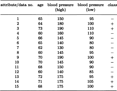
9.2. Find a decision tree that classifies the set of data shown in Exercise 9.1 into classes {+, −} that maximizes the amount of information in the sense of (9.4).
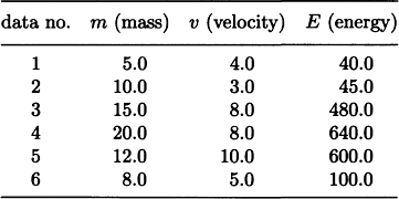
9.3. Using the method shown in Section 9.5(a), discover regularities in the following set of data (each datum gives the energy E that a wall receives when an object with mass m hits the wall at velocity v).
*In statistics, the former error is generally called an error of the first kind and the latter error is called an error of the second kind, from the standpoint of class 0.
*That a natural number n is a number with the maximal number of divisors means that ![]() where #(n) is the number of natural numbers that divides n. 1,2,4,6,12,… are numbers with a maximal number of divisors.
where #(n) is the number of natural numbers that divides n. 1,2,4,6,12,… are numbers with a maximal number of divisors.