
Learning Concepts
This chapter will discuss algorithms for learning concepts from examples. Learning concepts is the most basic kind of learning on a computer, so we need to understand it fully. We will first give the definition of a concept and general methods of learning concepts and algorithms. We will then give algorithms for version space and concept clustering.
6.1 Definition of a Concept
(a) Extensional and intensional meanings
Words such as “a triangle,” “a coffee cup,” and “a hammer” indicate a concept. An individual triangle is considered to be an example of the concept called a triangle. It is important to know how various concepts and their examples are represented in a computer when we formulate algorithms for pattern recognition and learning on a computer. In previous chapters, we represented a concept and its examples using representation techniques like class and instance; however, there we hardly defined terms such as concept and example. So, let us first define the notion of a concept.
There are two different ways of defining the meaning of a concept: extensional meaning and intensional meaning.
Definition 1
(extensional meaning) Various examples exist first and the meaning of a concept is defined by the set of these examples. This is the extensional meaning of a concept.
Definition 2
(intensional meaning) Various properties exist first and the meaning of a concept is defined by a set of these attributes. This is the intensional meaning of a concept.
Suppose we collect together all the triangles we have seen or have imagined and make the set of them. The extensional meaning of the concept “triangle” is this set. The intensional meaning of “triangle” is the set of its properties such that a triangle is surrounded by three line segments or that it is a plane figure. The extensional meaning and the intensional meaning of the same object are not necessarily the same. For example, “the brightest star in the evening (the evening star)” and “the brightest star in the morning (the morning star)” mean the same thing, Venus, in their extensional meaning, but they are different in their intensional meaning.
When we try to define a concept using extensional meaning, we need to list all its examples (it is impossible in an actual life but is possible conceptually). Using the intensional meaning, we can define a concept as a list of attributes, but, once again in real life, it is impossible to list all the possible attributes of a concept. In this book, we determine a set of attributes first and consider objects that satisfy such a set as examples of the concept. This type of definition can be considered as an approximation of a definition for the meaning of a concept that is both extensional and intensional.
The word “concept,” like “knowledge” and “learning,” has been used in philosophy and psychology. Although it is important to know the meaning of “concept” in these fields, we limit ourselves to the above approximate definition when we are dealing with learning on a computer.
(b) Representing a concept
A typical method for representing the meaning of a concept is to use a list containing the name of the concept followed by elements that are attribute-value pairs:
For example, the concept c “something big, red, and round,” can be expressed as follows using the three attributes, size, color, shape:
where size, color, and shape are the attributes representing a size, a color, and a shape, respectively, and large, red, and round are the values representing big, red, and round, respectively.
On the other hand, we also can represent the meaning of a concept using first-order predicate logic. In this case, each attribute corresponds to a predicate symbol and the name of the concept and the value correspond to arguments of the predicate. If we use the conjunction operator, a concept can generally be represented as a logical conjunction:
When a variable symbol is included in the above well-formed formula, the variable symbol is considered to be bound by the universal quantifier, ∀. If we omit the conjunction operators for simplicity, the definition of a concept can be represented as follows:
We also assume that the variable symbols in this set are bounded by universal quantifiers.
As an example, let us consider the concept c, “something big, red, and round.” If the predicate symbols for size, color, and shape are size, color, and shape, c can be represented as follows:
where large, red, and round are the constant symbols for big, red, and round, respectively. If we consider c, which we used as the name of the concept, to be a variable and use a variable symbol X, then the concept “something big, red, and round” can be represented by the well-formed formula
In this chapter, we will use a predicate logic representation for concepts unless otherwise noted.
The definition of a concept in predicate logic can vary depending on which logical operators we choose to combine predicates. We often use literals instead of general predicates to define a concept:
Definition 3
(a single concept) Suppose p1,…, pm are literals. Then P = P1 ⋀. .⋀pm, in other words, a concept defined by the logical conjunction of literals, is called a simple concept or a conjunctive concept. A simple concept is sometimes represented as a set of literals such as p = {p1,…, pm}
Definition 4
(multiple concepts) Suppose q1,…, qn are simple concepts. Then q = q1 ∨ … ∨ qn, in other words, a concept defined by the logical disjunction of concepts, is called a multiple concept or a disjunctive concept
The predicate logic representation of “something big, red, and round” is an example of a simple concept, “something big and red or small and blue” is a multiple concept and can be represented as
Besides these two kinds of concepts, there are also exclusive multiple concepts that combine simple concepts using the exclusive disjunction operator, and implicative concepts that combine concepts by an implication symbol. These concepts are not used often since their logical meaning is simple. In this book, unless otherwise noted, we will mean a simple concept when we say a concept.
(c) A concept and its instances
We can generate various instances of a concept by substituting constants for variable symbols in the definition of the concept. Let us look at the relationship between a concept and its instances. We will define an instance later in Definition 5.
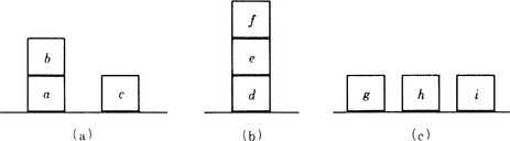
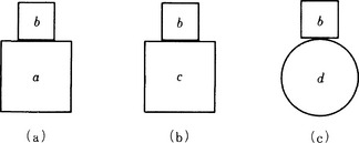
First, let us look at a figure shown in Figure 6.1. Suppose we have six literals
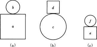
where the domain of each variable is
The conjunction of the literals
is the simple concept “two things with some kind of shape, size, and position.” Each of the three figures shown in Figure 6.1 can be regarded as representing an instance of the concept p. This is because each figure (a), (b), (c) corresponds to one of the logical expressions
that are obtained from p by applying the substitutions
Let us look at another example. Suppose, of the above six literals, we take only P2 and p3. Their conjunction is
The expression
that can be obtained by applying the substitution
to p′ is the concept meaning “something big is in a lower position.” Now, consider the substitutions ![]() and
and ![]() Then pθ1, pθ2 are special cases of the logical expressions
Then pθ1, pθ2 are special cases of the logical expressions
respectively.
contradicts pξ1.
The conjunction of literals which is an instance obtained by applying substitutions to an original concept is called a positive instance of the original concept. A conjunction of literals which is not a positive instance is called a negative instance of the original concept. pθ1, pθ2 and pξ1 are positive instances of the concept p, and p′ητ1, p′ητ2, and p′ητ3 are positive instances of p′η. pθ1 and pθ2 are positive instances of p′, but pξ1 is a negative instance of p′. Also, size(a, large) Λ position(a, upper) is a negative instance of p′. We will define positive and negative instances more accurately in Definition 5 below.
Next, let us pay attention to the fact that there are generally many concepts that have some particular conjunction of literals as a positive or negative instance. For example, for the substitution
p′η and pζ are both concepts that have pθ1 and pθ2 as positive instances and have pξ1 as a negative instance.
Although it is true that a positive (negative) instance of pζ always is a positive (negative) instance of p′η, the reverse is not true, because when we look at the concepts p and p′ as a set of literals, we have p′ ⊂ p and we have η ⊂ ζ for the substitution. In other words, the concepts associated with some particular instance are divided into more general concepts and more specific concepts depending on how we make conjunction and substitution.
To summarize what we have explained so far, let us now define an instance of a concept.
Definition 5
(positive instance and negative instance) We represent a concept, p, as the set, {p1,…,pn}, of literals constituting the concept. Suppose q is a finite set of ground literals. If ![]() holds for some substitution θ that replaces all the variable symbols included in p with constant symbols, we say that q is a positive instance of p. On the other hand, when r is a finite set of ground literals, if
holds for some substitution θ that replaces all the variable symbols included in p with constant symbols, we say that q is a positive instance of p. On the other hand, when r is a finite set of ground literals, if ![]() is true for any substitution ξ that replaces all the variable symbols with constant symbols, we say that r is a negative instance of p. We put together a positive instance and a negative instance and call them an instance. Also, when the above conditions pθ ⊂ q and
is true for any substitution ξ that replaces all the variable symbols with constant symbols, we say that r is a negative instance of p. We put together a positive instance and a negative instance and call them an instance. Also, when the above conditions pθ ⊂ q and ![]() are replaced by q
are replaced by q ![]() pθ and r
pθ and r ![]() pξ, respectively, we sometimes call q and r a positive instance and a negative instance of p, respectively.
pξ, respectively, we sometimes call q and r a positive instance and a negative instance of p, respectively.
Definition 6
(generalization) Suppose we regard each of the given positive instances P1,…, pn as a set of literals. If there exists a set of literals, p, such that for all i = 1,…, n, p ⊆ piθi holds for some θi, a substitution that replaces constant symbols with variable symbols, we call p a generalization of the positive instances p1,…, pn (based on θ1,…, θn). If we want to emphasize that p is represented by the conjunction of its elements, we specifically say that p is a conjunctive generalization. We also call it a generalization if we replace the conditions p ⊂ piθi by piθi ![]() p (i = 1,…,n).
p (i = 1,…,n).
We sometimes identify a concept whose positive instances are {p1,…, pn} with their generalization. There are usually many generalizations for a given set of positive instances of a concept. Each of those generalizations is one concept. When there are two generalizations pθ1 and pθ2 for the same set of positive instances, we determine which is more specific or more general using the following definition.
Definition 7
(specialization) We call pθ2 a specialization of pθ1 when pθ1 = pθ2ξ holds for some substitution ξ that replaces constant symbols with variable symbols. In this case we also say that pθ1 is a generalization of pθ2.
We will return to the generalization and specialization of concepts in Section 6.3.
6.2 Methods for Concept Learning
Here we will explain some methods for learning a concept from a given set of instances. These methods use algorithms that take a set of instances as input and output a concept. We need to be careful because there are generally many concepts that can be derived from the same set of well-formed formulas that make up a set of instances. So an algorithm for learning concepts cannot help but include heuristic evaluation of which concept to choose. Here, as the basic method of concept learning, we describe an application of heuristic search in problem solving.
(a) Information necessary for learning concepts
In this section we consider what is necessary in an algorithm for learning concepts. First, let us focus on what we mean by learning a concept.
Definition 8
(learning a concept) Suppose we have some positive instances p1,…, pm and negative instances q1,…, qn (m ≥ 0, n ≥ 0). We say we have learned a concept for the instances p1,…, pm, q1,…, qn if we have found a well-formed formula, r, for which there is a substitution θi (i = 1,…,m) that replaces constant symbols with variable symbols so that ![]() and for which there is no substitution ξj(j = 1,…, n) that replaces constant symbols with variable symbols so that r ⊆ qjξj (j = 1,…,n).
and for which there is no substitution ξj(j = 1,…, n) that replaces constant symbols with variable symbols so that r ⊆ qjξj (j = 1,…,n).
We say that r is a concept for the instances p1,…, pm, q1,…, qn. Learning a concept for a set of instances is called induction of the concept. Concept learning is learning by induction.
We need to pay attention to the following four things in order to improve the computational efficiency of learning concepts by a computer.
(1) Algorithms for learning concepts.
We will explain in subsection (b) algorithms for learning a concept from a given set of instances.
(2) Background knowledge and the introduction of new literals.
We need background knowledge to choose a specific concept for a given set of instances. We will explain in subsection (c) how we make use of such knowledge and how we make use of new literals when literals not included in the original set of instances appear in background knowledge.
(3) A set of instances and how they are given.
There are many ways in which a set of instances can be given to a system trying to learn a concept. For example, there are cases where only a small number of instances can be obtained or, to the contrary, where a large number of instances is given. There are cases where only positive instances are given. There are also cases where instances are obtained all at once or where they are obtained one by one.
A method that inputs all given instances at once into an algorithm for learning concepts is called simultaneous presentation; a method that inputs given instances one by one or incrementally is called incremental presentation. Simultaneous presentation is used, for example, in predicting weather from a large amount of given weather forecasting data. An example of this method is explained in Chapter 9. In an intelligent robot that is capable of learning, data for learning are usually obtained incrementally in real time. It is an example of incremental presentation.
We need to consider what representation language we can use to describe an instance and a concept. In this chapter, we use first-order predicate logic.
(b) Algorithms for learning concepts
Learning a concept from a given set of instances is generally done by replacing a constant included in the instance representation with a variable or by removing some literals from the instance. These transformations can be formalized as a problem solving process that involves generating and transforming predicates using some heuristic rules to obtain an appropriate well-formed formula. Let us define learning a concept as a problem solving process.
Definition 9
(problem solving) Suppose we have a set of positive instances, ET, a set of negative instances EF, and a set of rules, O, for transforming one well-formed formula to another. In the state space, S, where a set of well-formed formulas corresponds to a state, a rule o ∈ O can be considered to be a state transition rule on S. When we move through S to state s ∈ S using a rule o ∈ O, both ![]() and
and ![]() can be used as a constraint G, where θ and ξ are substitutions for replacing variable symbols with constant symbols. If we let c be the concept we are trying to find, then solving the problem P = 〈 S,O, G, ET, {c}〉 is called learning the concept c.
can be used as a constraint G, where θ and ξ are substitutions for replacing variable symbols with constant symbols. If we let c be the concept we are trying to find, then solving the problem P = 〈 S,O, G, ET, {c}〉 is called learning the concept c.
Although the concept c itself is used in the above definition, the structure of c is not usually known beforehand. Also, not all the elements of the state space S are known. So, in order to solve a problem P, we need to start from an initial state ET, apply a state transition rule to the current state, and generate a new state. By repeating this operation, if we find among the generated states a concept c for the original set of instances, we stop the search. In the problem solving framework, this can be done using an algorithm for heuristic search.
As an example, let us look at the three instances shown in Figure 6.2:
where p1 and p2 are positive instances and p3 is a negative instance.
We regard ET = {p1,p2} as the initial state and O = {o1, o2} as the set of state transition rules:
o1: (a rule for changing a constant into a variable)
Let p be one of the well-formed formulas included in the current state s ∈ S and p′ be the new well-formed formula obtained by replacing a constant symbol (or constant symbols) in p with a variable symbol (or variable symbols). In this case, the new state s′ ∈ S generated from s is s′ = s ∪ {p′} − {p}.
o2: (a rule for removing literals)
When q is one of the well-formed formulas included in the current state s ∈ S, we can obtain a new well-formed formula q′ by removing one of the literals in q. In this case, the new state s′ ∈ S generated from s is s′ = s ∪ {q′} − {q}.
First, let us apply the rule o1 to the state ET− For example, if we apply the substitution θ1 = {X/a} to p1 ∈ ET, we get the following state s1:
Now, for state s1, we have ![]() , so the state transition from ET to s1 satisfies the constraint. Next, we apply rule o1 to s1. For example, if we apply the substitution θ2 = {X/e} to
, so the state transition from ET to s1 satisfies the constraint. Next, we apply rule o1 to s1. For example, if we apply the substitution θ2 = {X/e} to ![]() ∈ s1 we obtain the following state, s2:
∈ s1 we obtain the following state, s2:
This state also satisfies the constraint. Now, let us apply the rule o2 to the state s2. For example, if we remove the literal on(X, d) included in ![]() , we obtain the following state that satisfies our constraint:
, we obtain the following state that satisfies our constraint:
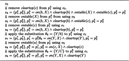
Furthermore, if we apply the rules in the order shown in Table 6.1 and continue with state transitions that satisfy our constraint, we finally obtain ![]() cleartop(Y). This c is, according to Definition 9, a concept for the instances p1, p2, and p3.
cleartop(Y). This c is, according to Definition 9, a concept for the instances p1, p2, and p3.
This example shows heuristic search in only one direction. Generally, more than one concept can be found by induction from a given set of instances, but this example does not cover the problem of how to choose one of the multiple concepts found by search. We will discuss this problem in Section 6.3.
(c) Background knowledge and introduction of new literals
There are cases when we can use background knowledge that includes literals not contained in instances. For example, suppose we have the background knowledge M
about the sample problem shown in Figure 6.2. Now if, from p1 and p2, we conclude
then {p1} ∪ M ![]()
![]() and {p2} ∪ M
and {p2} ∪ M![]()
![]() become true. So, if we repeatedly apply rules o2 and o1 to states, starting from the initial state {
become true. So, if we repeatedly apply rules o2 and o1 to states, starting from the initial state {![]() ,
,![]() } and paying attention to the negative instance p3, we can obtain tower(Y, X ) as a concept.
} and paying attention to the negative instance p3, we can obtain tower(Y, X ) as a concept.
Background knowledge is often useful for improving the efficiency of search; however, background knowledge can include literals that are not part of the original instances, as in the above example. Learning in which a new literal that does not appear in the original set of instances is included in the generated concept is called constructive learning of a concept. Learning that does not involve new literals is called selective learning of a concept.
6.3 Generalization of Well-Formed Formulas
The transition rules, o1,o2, for well-formed formules described in Section 6.2(b) are considered to be rules that generalize a well-formed formula. In this section, we will discuss the generalization of well-formed formulas, which is one of the most important problems in concept learning.
(a) MSC generalization
Let us look at the example in Figure 6.3. The three instances in Figure 6.3 can be represented as follows:
Now, let us consider four concepts
for which p1, p2, and p3 are positive instances. In c1 and c2, the number of literals is the same, but the number of variables in c2 is larger. The number of literals in c3 is smaller than the number of literals in c1. As you can see, there are differences in degree in the generalization and specialization of a concept for some given set of instances. We have already defined generalization and specialization in Definitions 6 and 7. Usually, we are interested in the most specific concepts for a given set of instances. We will explain what “the most specific” generalization is.
Let us look at generalization in the sense of Definition 6. Using the example in Figure 6.3, any one of c1,…, c4 is a generalization of p1, p2, and p3. For example, for c2, if we use the substitutions
the following is true:
Next, based on the definition of generalization given in Definition 6, we can define “the most specific” generalization.
Definition 10
(MSC generalization) Let p be the generalization obtained by applying substitutions θ1,…, θn to a given set of positive instances {p1,…, pn}. Then, if there do not exist substitutions ξi,ρi (i = 1,…, n) that replace constant symbols with variable symbols and a generalization p′ of {p1,…, pn} such that ![]() we call p an MSC generalization (maximally specific conjunctive generalization) of p1,…, pn.
we call p an MSC generalization (maximally specific conjunctive generalization) of p1,…, pn.
For example, in the previous example, if we consider c1,…, c4, p1,p2,p3 each as a set of literals, then there do not exist substitutions ξi,ρi {i = 1,2,3) and a generalization c′ where c1 = piθi (i = 1,2,3) for the following substitutions and θi (i − 1,2,3) and ![]() :
:
Therefore, c1 is an MSC generalization of p1, p2, and p3. On the other hand, c2,c3,c4 are not MSC generalizations of p1, p2, and p3. Even though an MSC generalization can be regarded as the most specific generalization, it is not always uniquely determined. However, since learning a concept often requires finding a concept that generalizes the set of instances as specifically as possible (for example, to include as few variables as possible), we usually choose one of the MSC generalizations from all the generalizations.
(b) Methods of generalization
In this section we provide methods for generalizing well-formed formulas. Rule o1 described in Section 6.2(b) can be considered a special case of the method described below.
(1) Changing a constant into a variable
This method replaces a constant symbol in a well-formed formula with a variable symbol. For example, if we consider the substitutions
for the two well-formed formulas
we will obtain the following generalization of q1 and q2:
(2) Generalization of a constant in a given structure
If relations among constants are given by a semantic network that inherits the characteristics of predicates, we can make a generalization by replacing a constant by another constant that corresponds to a node above the nodes of the original constants in the semantic network. For example, if the relations among square, triangle, and polygon are given by the semantic network shown in Figure 6.4, then for
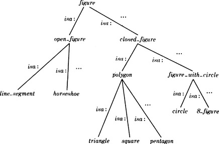
by replacing the nodes square and triangle with their parent node polygon, we can obtain the generalization
(3) Removing a literal included in a well-formed formula
When a well-formed formula is a conjunction of more than one literal, remove one or some number of literals. For example, let
(4) Deductive transformation of part of a well-formed formula
Replace some of the literals in a well-formed formula with a literal that can be deduced from those literals and, if available, background knowledge. For example, if, as background knowledge, we can use the formula
we can generalize the expression
to the following:
(Here we use the fact that we can prove q from p and the background knowledge.)
(5) Generalization using resolution
Simplifying a well-formed formula by using the inference rule ![]() , for any well-formed formulas p, q1, and q2, is called resolution. (The notion of resolution we described in Section 3.7 is an example of this kind of resolution.) Using resolution, we can generalize a given well-formed formula. For example, by extending the above rule a little, we obtain (p Λ q1 → r) Λ (∼p Λ q2 → r) → (q1 ν q2 → r) for any well-formed formula p, q1, q2, r. Using this rule, for example, on the well-formed formula
, for any well-formed formulas p, q1, and q2, is called resolution. (The notion of resolution we described in Section 3.7 is an example of this kind of resolution.) Using resolution, we can generalize a given well-formed formula. For example, by extending the above rule a little, we obtain (p Λ q1 → r) Λ (∼p Λ q2 → r) → (q1 ν q2 → r) for any well-formed formula p, q1, q2, r. Using this rule, for example, on the well-formed formula
produces the following generalization:
This is an example of a multiple concept rather than a simple concept.
By using this method as a state transition rule for learning concepts as described in Section 6.2(b), we can mechanically obtain a concept for a given set of instances. The above method, however, is a heuristic method and does not guarantee that we can always find an MSC generalization.
6.4 Version Space
As we described above, there may be many concepts for a given set of instances. To find these concepts, we can use heuristic search. Here, as an effective method for improving the efficiency of heuristic search, we will explain the method of version space, a search method that depends on the structure of the state space.
(a) An example of version space
Suppose we have four predicates representing the attributes of an object u:
We consider the following concepts, represented by a set of these predicates:
Now we leave the variable U in P1,P2,P3 as is and either substitute the constant symbol triangle, small, white, fine into W, X, Y, Z or leave W, X, Y, Z as is. We let Q be the set of concepts generated from P1,P2,P3- For example, the well-formed formula
that can be obtained by replacing W and X of P2 with triangle and small, respectively, is an element of Q. In this case, the number of elements in Q is 24 = 16. Now, we represent the elements of Q using a bit array of four 0s or 1s and let each bit correspond to one of the predicates shape, size, color, and texture. If a constant symbol has been substituted for one of the variables, W, X, Y, Z, then we make the corresponding bit 1; and if it stays as a variable symbol, we make it 0. For example, the formula p′2 is represented by 1101.
Using this representation, the relations among the elements of Qs can be represented by the graph shown in Figure 6.5, where each edge in the graph represents a substitution, the top node n1 represents the most “specific” concept, and the lowest node n3 represents the most “general” concept.
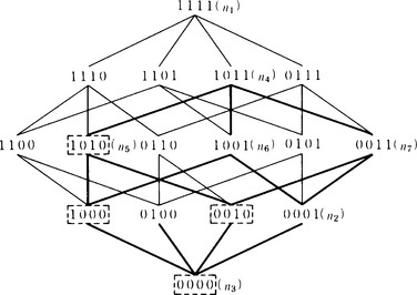
Edges or paths in the graph shown in Figure 6.5 represent substitutions. More concretely, the graph corresponds to a generalization of a well-formed formula by making constants into variables. For example, n3 is a generalization of n1, and n2 is a generalization of n1. A version space, intuitively, is a set of well-formed formulas that are related each other by generalizations as exemplified in the graph in Figure 6.5.
(b) The partial order of generalizations and version space
To explain concept learning using version space, let us give a more exact definition to version space. First, notice the fact that, as we noted in Definition 6, a generalization orders two well-formed formulas. We can describe this more generally as follows:
Definition 11
(partial order of generalizations) Let Q be a set of well-formed formulas each defined by a conjunction of literals. For qi and qj ∈ Q, we write qi ≤ qj if and only if qi is a generalization of qj. Then ≤ is a partial order on Q.* We call ≤ the partial order of generalizations.
In Definition 11, an MSC generalization corresponds to a maximal element in the partial order of generalizations.
Next, let us define version space using the partial order of generalizations.
Definition 12
(version space) Suppose the partial order of generalizations, ≤, is defined for a set of concepts, Q, and Q is a complete lattice** under ≤. In particular, there are an element q ∈ Q (the minimum element) that makes q ≤ qi and q < qj true and an element q′ ∈ Q (the maximum element) that makes qi ≤ q′ and qj ≤ q′ true for all qi,qj ∈ Q. We assume that the maximal element of the complete lattice Q corresponds to a given positive instance p. We call Qthe version space for the positive example p.
(c) Concept learning using the version space method
In a version space Q, relations among elements represent generalization relations among concepts. So we can narrow the search for a goal concept using the following rules:
(1) When a new positive example is given, only a concept obtained from that example or a concept that is more general than the example can be a goal concept.
(2) When a new negative example is given, no concept more general than the example can be the goal concept.
(3) Starting from the maximum element (the most specific case; in Figure 6.5, the top node) and the minimum element (the most general element; in Figure 6.5, the lowest node) of Q, we can narrow the possible subset including the goal concept using (1) and (2) together.
Finding a concept for a given set of examples using these rules is called concept learning by the version space method.
Let us use the version space method for the example in Figure 6.5. The concept
that is, “a white, fine-textured triangle,” is given as a new concept. Node n4 in Figure 6.5 corresponds to this concept. So, possible concepts that can be found by the version space method are n4 and the part of the graph connected by paths under n4. In Figure 6.5, this part is shown with bold lines.
in other words, “a white triangle,” is given as the concept corresponding to a negative instance. The node for this concept is n5 in Figure 6.5. Then the concept we are looking for does not exist in the part of the graph that includes n5 and that is connected by paths under n5. That is, the nodes surrounded by broken lines cannot correspond to the concept we are looking for. Now, if
that is, “a fine-textured triangle” (node n6 in Figure 6.5), is the concept for a negative instance, n6, then n2 cannot be the concept we are looking for. So, the concept we want is narrowed down to just one:
This concept corresponds to node n7 in Figure 6.5.
This example uses a small graph, but the version space method can be applied to graphs with many more nodes. The method can be used even when the elements of the space, in other words, the well-formed formulas that are candidates for the goal concept, are not known beforehand. This is true since a node of a graph can be generated every time an instance is given. In summary, concept learning using the version space method has the following features:
(1) If the maximum element and the minimum element of a version space and a method of generalization are given, we do not need to know the structure of the space beforehand.
(2) Learning a concept is possible not only when instances are input simultaneously but also when they are given one by one.
(3) When a variable is included in each element of a version space, the amount of computation can be very large.
Of these features, (1) and (2) are the most important in real use. For (3), notice that many concept relations can be formulated using a version space that does not involve variables at all.
6.5 Conceptual Clustering
So far we have described methods for concept learning from a given set of instances. On the other hand, classifying instances by finding some relation among them and separating them into several clusters so that each cluster corresponds to a concept is also an important problem in concept learning. Classifying a given set of instances into clusters so that each cluster corresponds to a different concept is called conceptual clustering.
(a) Conceptual clustering using attributes
Let us consider a conceptual clustering method that classifies instances based on attributes. Suppose that there are n objects o1,…, on, and each has some attributes represented by m variables x1,…, xm. For example, there are eight automobiles o1,…, o8, and each has the values shown in Table 6.2 for the three attributes, speed x1 ∈ {high, medium, low}, color x2 ∈ {red, blue, green}, and price x3 ∈ {high, relatively-high, relatively-low, low}. Below, using this example problem, we will explain conceptual clustering.
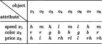
We now try to classify n given objects into several different clusters by whether their attribute-value pairs are similar or not. Suppose that the number of clusters k is given beforehand and that we have an evaluation function f that can tell us how close objects are (of course, this depends on the method of classification). Conceptual clustering by attributes can be characterized as classifying n objects into k different clusters so that the value of f is minimum. Let us look at Table 6.2. It can be rewritten as Figure 6.6 when based on attributes. Now, let us define the evaluation function f as follows:
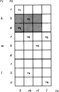
First, to determine the area surrounding some attribute-value pairs, we can specify part of the matrix shown in Figure 6.6. For example, ![]() specifies the gray area in Figure 6.6. An area around attribute-value pairs determined in this way is called an attribute complex. The number of matrix elements that are included in an attribute complex α, but do not contain an object, is called the sparseness of α and is written s(α). For example, the sparseness of the attribute complex corresponding to the gray part of Figure 6.6 is s(α) = 4. We can imagine that the higher the sparseness of an attribute complex is, the larger it will be as a cluster for classifying given objects. Suppose we have found a set of attribute complexes that can classify k objects, {α1,…, αk}, where αi (i = 1,…, k) is the attribute complex that separates the objects in the ith cluster from the other objects. We now define f as
specifies the gray area in Figure 6.6. An area around attribute-value pairs determined in this way is called an attribute complex. The number of matrix elements that are included in an attribute complex α, but do not contain an object, is called the sparseness of α and is written s(α). For example, the sparseness of the attribute complex corresponding to the gray part of Figure 6.6 is s(α) = 4. We can imagine that the higher the sparseness of an attribute complex is, the larger it will be as a cluster for classifying given objects. Suppose we have found a set of attribute complexes that can classify k objects, {α1,…, αk}, where αi (i = 1,…, k) is the attribute complex that separates the objects in the ith cluster from the other objects. We now define f as
Also, we agree that f is minimized over sets of attribute complexes that can classify k different objects. For example, in the problem in Figure 6.6, if we assume k = 2, conceptual clustering by attributes becomes the problem of finding two attribute complexes α1,α2 that divide o1,…, o8 into different clusters and that make f = s(α1) + s(α2) minimum.
Below, we will describe an algorithm for solving this kind of problem. At the heart of this algorithm is a clustering algorithm for dividing a set of objects into k clusters. By applying it recursively, we can generate a representation where clusters are hierarchically structured. Below we will show an algorithm for clustering including an algorithm for generating a cluster hierarchy. By a cover of a set of objects O, we mean a set of sets α = {Q1, …, Qm} that satisfies the property ![]() . Also, if
. Also, if ![]() hold for a cover of the set O, α = {Q1,…, Qm}, {O1,…, Om} is called a partition of O by the cover α.
hold for a cover of the set O, α = {Q1,…, Qm}, {O1,…, Om} is called a partition of O by the cover α.
Algorithm 6.1
(conceptual clustering by attributes)
[1] Let I be the upper limit of the number of iterations. Set iteration = 1, ![]() . (Setting parameter values)
. (Setting parameter values)
[2] Extract k objects o1,…, ok from the given objects. (Extracting cluster seeds)
[3] Obtain a set of attribute complexes {αi1,…, αini} that distinguishes oi from o1, …, oi−1, oi+1, …, ok for each i (i = 1,…, k).
[4] For the attribute complexes obtained in [3]:
find ![]() (where
(where ![]() ranges over only the covers of {o1,…, ok}). If fmin ≤ f0, then set f0 = fmin. Pick one of
ranges over only the covers of {o1,…, ok}). If fmin ≤ f0, then set f0 = fmin. Pick one of ![]() that give fmin, and call it
that give fmin, and call it ![]() .Go to [5].If fmin≤f0 then go to [6]. (Selecting an attribute complex that makes the evaluation function value minimum)
.Go to [5].If fmin≤f0 then go to [6]. (Selecting an attribute complex that makes the evaluation function value minimum)
[5] If iteration ≥ I, go to [6]. Otherwise, go to [7]. (Checking the number of iterations)
[6] Stop. The partition of {o1,…,ok} by the cover ![]() is a solution to the clustering. (Termination condition)
is a solution to the clustering. (Termination condition)
[7] Select one of the objects included in each of the k attribute complexes ![]() (i = 1,…, k), in
(i = 1,…, k), in ![]() , and call it oi (i = 1,…, k). These objects are selected by the following substeps. (Selecting new cluster seeds)
, and call it oi (i = 1,…, k). These objects are selected by the following substeps. (Selecting new cluster seeds)
[7.1] Do the following for each ![]() (i = 1,…, k). Let p be the vector of values for attributes of objects o in
(i = 1,…, k). Let p be the vector of values for attributes of objects o in ![]() . If there are two of these vectors, p and q, define the distance between p and q by the number of their elements that are not the same (called the Hamming distance). Obtain, as follows, the median vector
. If there are two of these vectors, p and q, define the distance between p and q by the number of their elements that are not the same (called the Hamming distance). Obtain, as follows, the median vector ![]() for the vectors, pj (j = i1,…,jnj), corresponding to objects included in
for the vectors, pj (j = i1,…,jnj), corresponding to objects included in ![]() :
:
For each dimension of the vector pj (j = i1,…,inj), pick the value that appears most often. Then let ![]() be the vector of those values.
be the vector of those values.
[7.2] Pick the vector that has the smallest Hamming distance to g(α^jii) from the vectors pj (j = i1,…, inj) corresponding to objects in ![]() (i = 1,…, k). Let the objects corresponding to this vector be the objects selected from
(i = 1,…, k). Let the objects corresponding to this vector be the objects selected from ![]() .
.
When all the objects were selected by the substeps, let iteration = iteration + 1 and go to [3].
[1] Divide the given objects into k clusters using the clustering algorithm. (Application of clustering)
[2] If the hierarchy of clusters reaches a given depth, stop. Otherwise, go to [3]. (Termination condition)
[3] Generate subclusters by applying [1] to each cluster generated in [1]. This increments the depth of the cluster hierarchy. Go to [2]. (Recursive application)
Let us apply the clustering algorithm to the example in Figure 6.6, where the upper limit of the number of iterations is set to 2.
[1] Let I = 2, iteration = 1, ![]() .
.
[2] Pick o1 and o2 from o1,…, o8 (which object is chosen influences the efficiency of the computation).
[3] Suppose we found the following attribute complexes that include o1 but do not include o2:
In this case, {o1,o4,o5,o7,o8} ∈ α11 and {o1,p3,o4,o6,o7} ∈ α12. Suppose we found the following attribute complexes that include o2 but do not include o1:
In this case, {o2,o3, o6} ∈ α12and {o2,o5, o8} ∈ α22 (There are many other sets of attribute complexes that satisfy the conditions, but we limit ourselves here to these two.)
[4] If we let ![]() for
for ![]() , only αA and αD are a cover of {o1,…, o8}. For these, using
, only αA and αD are a cover of {o1,…, o8}. For these, using
the minimum value of f is fmin = 22 and fmin < f0. The cover that gives fmin is αA, so let ![]() .
.
[5] Since iteration < 2, go to [7].
[7] The objects included in α11, o1, o4, o5, o7, o8, can be represented by the following three-dimensional vectors for the values of the attributes x1, x2, x3.
Then we can pick ![]() as the median vector. In this case, o7 is the object that is closest to g. Similarly, if we pick
as the median vector. In this case, o7 is the object that is closest to g. Similarly, if we pick ![]() as the median vector, we find that o6 is the object that is closest to g. Set iteration = 2.
as the median vector, we find that o6 is the object that is closest to g. Set iteration = 2.
[3] If we found the following attribute complexes that include o7 but do not include o6:
we have {o1, o3, o4, o7, o8} ![]() , and {o1, o4, o7, o8} ∈ α21. Also, if we found the following attribute complexes that include o6 but do not include o7:
, and {o1, o4, o7, o8} ∈ α21. Also, if we found the following attribute complexes that include o6 but do not include o7:
[4] For αA = {α11, α12},αB = {α21, α12} only αA is a cover of {o1, …, o8}. For αA we have
and ![]() since
since ![]() Go to [5].
Go to [5].
[5] Since iteration = 2, go to [6].
[6] Stop. The partition {o1, o3, o4, o7, o8}, {o2, o5, o6} by the cover ![]() is a solution of the clustering.
is a solution of the clustering.
The two clusters found in the above example turn out to be the cluster of the objects where the value of the attribute x3 is h or rh and the cluster of the objects where the value of the attribute x3 is rl or l.
The algorithm for conceptual clustering described here is a heuristic method and does not always find a clustering that makes f, the sum of the sparseness, minimum. However, not many conceptual clustering methods have been proposed where the clusters are unknown. Besides algorithms using the attribute values, as we described here, there are other conceptual clustering methods where the data are input one by one.
(b) Conceptual clustering and cluster analysis
Cluster analysis is a clustering method similar to conceptual clustering. Conceptual clustering is different from cluster analysis in that it classifies clusters according to the semantic structures of concepts. Cluster analysis cannot usually take global attributes of the data set into consideration, since it represents the value of an attribute of the data as a single number. On the other hand, conceptual clustering finds clusters based on the type of concepts it is given. Therefore, even if the distance between two objects is small in the sense of cluster analysis, if the two objects are examples of different concepts, conceptual clustering can possibly do the classification.
When we think about classification based on concepts, the goal of the classification and background knowledge are necessary elements in the classification. Although we have not denned background knowledge, we can understand its importance. For example, even variables that are not included in the attribute descriptions of a given object can be used for clustering as long as the variables and the given attributes are related by background knowledge.
Summary
In this chapter, we defined the notion of concept and its instances. We also described algorithms for learning concepts.
6.1. (Simple) concepts can be defined by the conjunction of literals, and their instances can be obtained as the conjunction of ground literals where constant symbols are substituted into variable symbols in a concept.
6.2. To learn concepts, we need to decide on an algorithm, background knowledge and its representation, a method for introducing new literals, a set of instances and a way to input them, and a method of representing instances and concepts.
6.3. Learning concepts can be done by generalizing well-formed formulas. Generalization of well-formed formulas is based on the notion of MSC generalization. Generalization can be done by heuristically applying methods like replacing constant symbols with variable symbols and applying deductive transformation.
6.4. Concept learning can be done based on an algorithm for heuristic search in problem solving. A popular method of this kind is the version space method.
6.5. One algorithm for conceptual clustering is to classify a set of instances into exclusive clusters, each corresponding to a different concept.
Exercises
6.1. Enumerate decisions that you have to make when learning concepts on a computer.
6.2. For the example problem (Figure 6.1) in Section 6.1(c), consider the conjunction of literals
and the substitution
Then show that p″ and n″ are concepts for the positive instances ![]() ,
, ![]() and the negative instance pξ1.
and the negative instance pξ1.
6.3. Find an MSC generalization of positive instances:

Also, give an example of a generalization that is not an MSC generalization. Furthermore, check if the found MSC generalization is an overgeneralization according to our knowledge. If so, devise a method for improving it.
6.4. Write a learning algorithm for integration by parts of indefinite integrals using the version space method.
*For a given set A and a binary relation ≤ on the elements of A, ≤ is a partial order on A if and only if the reflection law (ai ≤ ai), the symmetry law (if ai ≤ aj and aj ≤ ai, then ai = aj), and the transitive law (if ai ≤ aj and aj ≤ ak, then ai ≤ ak) are true for all ai, aj, ak ∈ A. For aj ∈ A, if ai ≤ aj is true for all ai ∈ A where aj ≠ ai, then aj is called a maximal element of the partial order ≤. If aj ∈ A and if aj ≥ ai is true for all aj ≠ ai, then ai is a minimal element.
**If, for each subset D of a partially ordered set Q, there exist q and q′ such that q ≤ qi and qi ≤ q′ for all qi ∈ D, then we say that Q is a complete lattice. We call q and q′ a lower bound and an upper bound of D, respectively. When D = Q, we call them the minimum and maximum elements of Q.