
Chapter 9
Parallel Patterns: Prefix Sum
An Introduction to Work Efficiency in Parallel Algorithms
Chapter Outline
9.1 Background
9.2 A Simple Parallel Scan
9.3 Work Efficiency Considerations
9.4 A Work-Efficient Parallel Scan
9.5 Parallel Scan for Arbitrary-Length Inputs
9.6 Summary
9.7 Exercises
Our next parallel pattern is prefix sum, which is also commonly known as scan. Parallel scan is frequently used to convert seemingly sequential operations, such as resource allocation, work assignment, and polynomial evaluation, into parallel operations. In general, if a computation is naturally described as a mathematical recursion, it can likely be parallelized as a parallel scan operation. Parallel scan plays a key role in massively parallel computing for a simple reason: any sequential section of an application can drastically limit the overall performance of the application. Many such sequential sections can be converted into parallel computation with parallel scan. Another reason why parallel scan is an important parallel pattern is that sequential scan algorithms are linear algorithms and are extremely work-efficient, which makes it also very important to control the work efficiency of parallel scan algorithms. As we will show, a slight increase in algorithm complexity can make parallel scan run slower than sequential scan for large data sets. Therefore, work-efficient parallel scan also represents an important class of parallel algorithms that can run effectively on parallel systems with a wide range of available computing resources.
9.1 Background
Mathematically, an inclusive scan operation takes a binary associative operator ⊕, and an input array of n elements [x0, x1, …, xn−1], and returns the output array
[x0, (x0 ⊕ x1), …, (x0 ⊕ x1 ⊕ … ⊕ xn−1)]
For example, if ⊕ is addition, then an inclusive scan operation on the input array [3 1 7 0 4 1 6 3] would return [3 4 11 11 15 16 22 25].
We can illustrate the applications for inclusive scan operations using an example of cutting sausage for a group of people. Assume that we have a 40-inch sausage to be served to eight people. Each person has ordered a different amount in terms of inches: 3, 1, 7, 0, 4, 1, 6, 3. That is, person number 0 wants 3 inches of sausage, person number 1 wants 1 inch, and so on. We can cut the sausage either sequentially or in parallel. The sequential way is very straightforward. We first cut a 3-inch section for person number 0. The sausage is now 37 inches long. We then cut a 1-inch section for person number 1. The sausage becomes 36 inches long. We can continue to cut more sections until we serve the 3-inch section to person number 7. At that point, we have served a total of 25 inches of sausage, with 15 inches remaining.
With an inclusive scan operation, we can calculate all the cutting points based on the amount each person orders. That is, given an addition operation and an order input array [3 1 7 0 4 1 6 3], the inclusive scan operation returns [3 4 11 11 15 16 22 25]. The numbers in the return array are cutting locations. With this information, one can simultaneously make all the eight cuts that will generate the sections that each person ordered. The first cut point is at the 3-inch point so the first section will be 3 inches, as ordered by person number 0. The second cut point is 4, therefore the second section will be 1-inch long, as ordered by person number 1. The final cut will be at the 25-inch point, which will produce a 3-inch long section since the previous cut point is at the 22-inch point. This gives person number 7 what she ordered. Note that since all the cutting points are known from the scan operation, all cuts can be done in parallel.
In summary, an intuitive way of thinking about inclusive scan is that the operation takes an order from a group of people and identifies all the cutting points that allow the orders to be served all at once. The order could be for sausage, bread, campground space, or a contiguous chunk of memory in a computer. As long as we can quickly calculate all the cutting points, all orders can be served in parallel.
An exclusive scan operation is similar to an inclusive operation with the exception that it returns the output array
[0, x0, (x0 ⊕ x1), …, (x0 ⊕ x1 ⊕ … ⊕ xn−2)]
That is, the first output element is 0 while the last output element only reflects the contribution of up to xn−2.
The applications of an exclusive scan operation are pretty much the same as those for an inclusive scan. The inclusive scan provides slightly different information. In the sausage example, the exclusive scan would return [0 3 4 11 11 15 16 22], which are the beginning points of the cut sections. For example, the section for person number 0 starts at the 0-inch point. For another example, the section for person number 7 starts at the 22-inch point. The beginning point information is important in applications such as memory allocation, where the allocated memory is returned to the requester via a pointer to its beginning point.
Note that it is fairly easy to convert between the inclusive scan output and the exclusive scan output. One simply needs to do a shift and fill in an element. When converting from inclusive to exclusive, one can simply shift all elements to the right and fill in value 0 for the 0 element. When converting from exclusive to inclusive, we need to shift all elements to the left and fill in the last element with the previous last element plus the last input element. It is just a matter of convenience that we can directly generate an inclusive or exclusive scan, whether we care about the cutting points or the beginning points for the sections.
In practice, parallel scan is often used as a primitive operation in parallel algorithms that perform radix sort, quick sort, string comparison, polynomial evaluation, solving recurrences, tree operations, and histograms.
Before we present parallel scan algorithms and their implementations, we would like to first show a work-efficient sequential inclusive scan algorithm and its implementation. We will assume that the operation is addition. The algorithm assumes that the input elements are in the x array and the output elements are to be written into the y array.
void sequential_scan(float ∗x, float ∗y, int Max_i) {
y[0] = x[0];
for (int i = 1; i < Max_i; i++) {
y[i] = y [i-1] + x[i];
}
}
The algorithm is work-efficient. With a reasonably good compiler, only one addition, one memory load, and one memory store are used in processing each input x element. This is pretty much the minimal that we will ever be able to do. As we will see, when the sequential algorithm of a computation is so “lean and mean,” it is extremely challenging to develop a parallel algorithm that will consistently beat the sequential algorithm when the data set size becomes large.
9.2 A Simple Parallel Scan
We start with a simple parallel inclusive scan algorithm by doing a reduction operation for all output elements. The main idea is to create each element quickly by calculating a reduction tree of the relevant input elements for each output element. There are multiple ways to design the reduction tree for each output element. We will present a simple one that is shown in Figure 9.1.
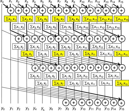
Figure 9.1 A simple but work-inefficient parallel inclusive scan.
The algorithm is an in-place scan algorithm that operates on an array XY that originally contains input elements. It then iteratively evolves the contents of the array into output elements. Before the algorithm begins, we assume XY[i] contains input element xi. At the end of iteration n, XY[i] will contain the sum of 2n input elements at and before the location. That is, at the end of iteration 1, XY[i] will contain xi−1+xi and at the end of iteration 2, XY[i] will contain xi-3+xi−2+xi−1+xi, and so on.
Figure 9.1 illustrates the algorithm with a 16-element input example. Each vertical line represents an element of the XY array, with XY[0] in the leftmost position. The vertical direction shows the progress of iterations, starting from the top of the figure. For the inclusive scan, by definition, y0 is x0 so XY[0] contains its final answer. In the first iteration, each position other than XY[0] receives the sum of its current content and that of its left neighbor. This is illustrated by the first row of addition operators in Figure 9.1. As a result, XY[i] contains xi−1+xi. This is reflected in the labeling boxes under the first row of addition operators in Figure 9.1. For example, after the first iteration, XY[3] contains x2+x3, shown as ∑x2..x3. Note that after the first iteration, XY[1] is equal to x0+x1, which is the final answer for this position. So, there should be no further changes to XY[1] in subsequent iterations.
In the second iteration, each position other than XY[0] and XY[1] receive the sum of its current content and that of the position that is two elements away. This is illustrated in the labeling boxes below the second row of addition operators. As a result, XY[i] now contains xi−3+xi−2+xi−1+xi. For example, after the first iteration, XY[3] contains x0+x1+x2+x3, shown as ∑x0..x3. Note that after the second iteration, XY[2] and XY[3] contain their final answers and will not need to be changed in subsequent iterations.
Readers are encouraged to work through the rest of the iterations. We now work on the implementation of the algorithm illustrated in Figure 9.1. We assign each thread to evolve the contents of one XY element. We will write a kernel that performs a scan on a section of the input that is small enough for a block to handle. The size of a section is defined as a compile-time constant SECTION_SIZE. We assume that the kernel launch will use SECTION_SIZE as the block size so there will be an equal number of threads and section elements. All results will be calculated as if the array only has the elements in the section. Later, we will make final adjustments to these sectional scan results for large input arrays. We also assume that input values were originally in a global memory array X, the address of which is passed into the kernel as an argument. We will have all the threads in the block to collaboratively load the X array elements into a shared memory array XY. At the end of the kernel, each thread will write its result into the assigned output array Y.
__global__ void work_inefficient_scan_kernel(float ∗X, float ∗ Y,
int InputSize) {
__shared__ float XY[SECTION_SIZE];
int i = blockIdx.x∗blockDim.x + threadIdx.x;
if (i < InputSize) {
XY[threadIdx.x] = X[i];
}
// the code below performs iterative scan on XY
…
Y[i] = XY[threadIdx.x];
}
We now focus on the implementation of the iterative calculations for each XY element in Figure 9.1 as a for loop:
for (unsigned int stride = 1; stride <= threadIdx.x; stride ∗= 2) {
__syncthreads();
XY[threadIdx.x] += XY[threadIdx.x-stride];
}
The loop iterates through the reduction tree for the XY array position that is assigned to a thread. Note that we use a barrier synchronization to make sure that all threads have finished their current iteration of additions in the reduction tree before any of them starts the next iteration. This is the same use of __syncthreads(); as in the reduction discussion in Chapter 6. When the stride value becomes greater than a thread’s threadIdx.x value, it means that the thread’s assigned XY position has already accumulated all the required input values. Thus, the thread can exit the while loop. The smaller the threadIdx.x value, the earlier the thread will exit the while loop. This is consistent with the example shown in Figure 9.1. The actions of the smaller positions of XY end earlier than the larger positions. This will cause some level of control divergence in the first warp when stride values are small. The effect should be quite modest for large block sizes since it only impacts the first loop for smaller stride values. The detailed analysis is left as an exercise. The final kernel is shown in Figure 9.2.
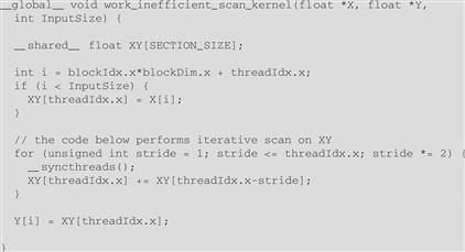
Figure 9.2 A kernel for the inclusive scan algorithm in Figure 9.1.
We can easily convert an inclusive scan kernel to an exclusive scan kernel. Recall that an exclusive scan is equivalent to an inclusive scan with all elements shifted to the right by one position and element 0 filled with value 0. This is illustrated in Figure 9.3. Note that the only real difference is the alignment of elements on top of the picture. All labeling boxes are updated to reflect the new alignment. All iterative operations remain the same.
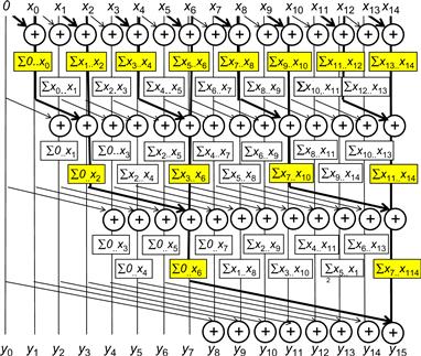
Figure 9.3 Work-inefficient parallel exclusive scan.
We can now easily convert the kernel in Figure 9.2 into an exclusive scan kernel. The only modification we need to do is to load 0 into XY[0] and X[i-1] into XY[threadIdx.x], as shown in the following code:
if (i < InputSize && threadIdx.x != 0) {
XY[threadIdx.x] = X[i-1];
} else {
XY[threadIdx.x] = 0;
}
Note that the XY positions of which the associated input elements are outside the range are now also filled with 0. This causes no harm and yet it simplifies the code slightly. We leave the work to finish the exclusive scan kernel as an exercise.
9.3 Work Efficiency Considerations
We now analyze the work efficiency of the kernel in Figure 9.2. All threads will iterate up to log(N) steps, where N is the SECTION_SIZE. In each iteration, the number of threads that do not need to do any addition is equal to the stride size. Therefore, we can calculate the amount of work done for the algorithm as
![]()
The first part of each term is independent of the stride, so they add up to N×log2(N). The second part is a familiar geometric series and sums up to (N − 1). So the total number of add operations is
![]()
Recall that the number of add operations for a sequential scan algorithm is N − 1. We can put this into perspective by comparing the number of add operations for different N values, as shown in Figure 9.4. Note that even for modest-size sections, the kernel in Figure 9.2 does much more work than the sequential algorithm. In the case of 1,024 elements, the kernel does nine times more work than the sequential code. The ratio will continue to grow as N becomes larger. Such additional work is problematic in two ways. First, the use of hardware for executing the parallel kernel needs to be much less efficient. In fact, just to break even one needs to have at least nine times more execution units in a parallel machine than the sequential machine. For example, if we execute the kernel on a parallel machine with four times the execution resources as a sequential machine, the parallel machine executing the parallel kernel can end up with only half the performance of the sequential machine executing the sequential code. Second, all the extra work consumes additional energy. This makes the kernel inappropriate for power-constrained environments such as mobile applications.
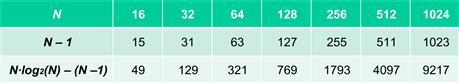
Figure 9.4 Work efficiency calculation for the kernel in Figure 9.2.
9.4 A Work-Efficient Parallel Scan
While the kernel in Figure 9.2 is conceptually simple, its work efficiency is too low for many practical applications. Just by inspecting Figures 9.1 and 9.3, we can see that there are potential opportunities for sharing some intermediate results to streamline the operations performed. However, to allow more sharing across multiple threads, we need to quickly calculate the intermediate results to be shared and then quickly distribute them to different threads.
As we know, the fastest parallel way to produce sum values for a set of values is a reduction tree. A reduction tree can generate the sum for N values in log2(N) steps. Furthermore, the tree can also generate a number of subsums that can be in the calculation of some of the scan output values.
In Figure 9.5, we produce the sum of all 16 elements in four steps. We use the minimal number of operations needed to generate the sum. During the first step, only the odd element of XY[i] will be changed to xi−1+xi. During the second step, only the XY elements of which the indices are of the form of 4×n − 1, which are 3, 7, 11, and 15 in Figure 9.5, will be updated. During the third step, only the XY elements of which the indices are of the form 8×n − 1, which are 7 and 15, will be updated. Finally, during the fourth step, only XY[15] is updated. The total number of operations performed is 8+4+2+1=15. In general, for a scan section of N elements, we would do (N/2)+(N/4) +…+ 2+1=N − 1 operations for this reduction phase.

Figure 9.5 Basic idea of a work-efficient parallel scan algorithm.
The second part of the algorithm is to use a reverse tree to distribute the partial sums to the positions that can use these values as quickly as possible. This is illustrated in the bottom half of Figure 9.5. At the end of the reduction phase, we have quite a few usable partial sums. For our example, the first row of Figure 9.6 shows all the partial sums in XY right after the top reduction tree. An important observation is that XY[0], XY[7], and X[15] contain their final answers. Therefore, all remaining XY elements can obtain the partial sums they need from no farther than four positions away. For example, XY[14] can obtain all the partial sums it needs from XY[7], XY[11], and XY[13]. To organize our second half of the addition operations, we will first show all the operations that need partial sums from four positions away, then two positions away, then one position way. By inspection, XY[7] contains a critical value needed by many positions in the right half. A good way is to add XY[7] to XY[11], which brings XY[11] to the final answer. More importantly, XY[7] also becomes a good partial sum for XY[12], XY[13], and XY[14]. No other partial sums have so many uses. Therefore, there is only one addition, XY[11]=XY[7]+XY[11], that needs to occur in the four-position level in Figure 9.5. We show the updated partial sum in the second row of Figure 9.6.
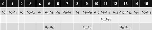
Figure 9.6 Partial sums available in each XY element after the reduction tree phase.
We now identify all additions for getting partial sums that are two positions away. We see that XY[2] only needs the partial sum that is next to it in XY[1]. This is the same with XY[4]—it needs the partial sum next to it to be complete. The first XY element that can need a partial sum two positions away is XY[5]. Once we calculate XY[5]=XY[3]+XY[5], XY[5] contains the final answer. The same analysis shows that XY[6] and XY[8] can become complete with the partial sums next to them in XY[5] and XY[7].
The next two-position addition is XY[9]=XY[7]+XY[9], which makes XY[9] complete. XY[10] can wait for the next round to catch XY[9]. XY[12] only needs the XY[11], which contains its final answer after the four-position addition. The final two-position addition is XY[13]=XY[11]+XY[13]. The third row shows all the updated partial sums in XY[5], XY[9], and XY[13]. It is clear that now every position is either complete or can be completed when added by its left neighbor. This leads to the final row of additions in Figure 9.5, which completes the contents for all the incomplete positions XY[2], XY[4], XY[6], XY[8], XY[10], and XY[12].
We could implement the reduction tree phase of the parallel scan using the following loop:
for (unsiged int stride = 1; stride < threadDim.x; stride ∗= 2) {
__synchthreads();
if ((threadIdx.x + 1)%(2∗stride) == 0) {
XY[threadIdx.x] += XY[threadIdx.x - stride];
}
}
Note that this loop is very similar to the reduction in Figure 6.2. The only difference is that we want the thread that has a thread index that is in the form of 2n − 1, rather than 2n to perform addition in each iteration. This is why we added 1 to the threadIdx.x when we select the threads for performing addition in each iteration. However, this style of reduction is known to have control divergence problems. A better way to do this is to use a decreasing number of contiguous threads to perform the additions as the loop advances:
for (unsigned int stride = 1; stride < blockDim.x; stride ∗= 2) {
__syncthreads();
int index = (threadIdx.x+1) ∗ 2∗ stride -1;
if (index < blockDim.x) {
XY[index] += XY[index - stride];
}
}
In our example in Figure 9.5, there are 16 threads in the block. In the first iteration, the stride is equal to 1. The first 8 consecutive threads in the block will satisfy the if condition. The index values calculated for these threads will be 1, 3, 5, 7, 9, 11, 13, and 15. These threads will perform the first row of additions in Figure 9.5. In the second iteration, the stride is equal to 2. Only the first 4 threads in the block will satisfy the if condition. The index values calculated for these threads will be 3, 7, 11, and 15. These threads will perform the second row of additions in Figure 9.5. Note that since we will always be using consecutive threads in each iteration, the control divergence problem does not arise until the number of active threads drops below the warp size.
The distribution tree is a little more complex to implement. We make an observation that the stride value decreases from SECTION_SIZE/2 to 1. In each iteration, we need to “push” the value of the XY element from a position that is a multiple of the stride value minus 1 to a position that is a stride away. For example, in Figure 9.5, the stride value decreases from 8 to 1. In the first iteration in Figure 9.5, we would like to push the value of XY[7] to XY[11], where 7 is 8−1. In the second iteration, we would like to push the values of XY[3], XY[7], and XY[11] to XY[5], XY[9], and XY[13]. This can be implemented with the following loop:
for (int stride = SECTION_SIZE/4; stride > 0; stride /= 2) {
__syncthreads();
int index = (threadIdx.x+1)∗stride∗2-1;
if(index + stride < BLOCK_SIZE) {
XY[index + stride] += XY[index];
}
}
The calculation of index is similar to that in the reduction tree phase. The final kernel for a work-efficient parallel scan is shown in Figure 9.7. Readers should notice that we never need to have more than SECTION_SIZE/2 threads for either the reduction phase or the distribution phase. So, we could simply launch a kernel with SECTION_SIZE/2 threads in a block. Since we can have up to 1,024 threads in a block, each scan section can have up to 2,048 elements. However, we will need to have each thread to load two X elements at the beginning and store two Y elements at the end. This will be left as an exercise.
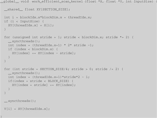
Figure 9.7 A work-efficient kernel for an inclusive scan.
As was the case of the work-inefficient scan kernel, one can easily adapt the work-efficient inclusive parallel scan kernel into an exclusive scan kernel with a minor adjustment to the statement that loads X elements into XY. Interested readers should also read [Harris 2007] for an interesting natively exclusive scan kernel that is based on a different way of designing the distribution tree phase of the scan kernel.
We now analyze the number of operations in the distribution tree stage. The number of operations are (16/8) − 1+(16/4)+(16/2). In general, for N input elements, the total number of operations would be (N/2)+(N/4) +…+ 4+2−1, which is less than N − 2. This makes the total number of operations in the parallel scan 2×N − 3. Note that the number of operations is now a proportional to N, rather than N×log2(N). We compare the number of operations performed by the two algorithms for N from 16 to 1,024 in Figure 9.8.
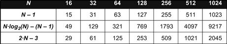
Figure 9.8 Work efficiency of the kernels.
The advantage of a work-efficient algorithm is quite clear in the comparison. As the input section becomes bigger, the work-efficient algorithm never performs more than two times the number of operations performed by the sequential algorithm. As long as we have at least two times more hardware execution resources, the parallel algorithm will achieve better performance than the sequential algorithm. This is not true, however, for the work-inefficient algorithm. For 102 elements, the parallel algorithm needs at least nine times the hardware execution resources just to break even.
9.5 Parallel Scan for Arbitrary-Length Inputs
For many applications, the number of elements to be processed by a scan operation can be in the millions. Obviously, we cannot expect that all input elements can fit into the shared memory. Furthermore, it would be a loss of parallelism opportunity if we used only one thread block to process these large data sets. Fortunately, there is a hierarchical approach to extending the scan kernels that we have generated so far to handle inputs of arbitrary size. The approach is illustrated in Figure 9.9.
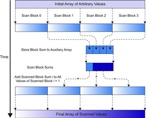
Figure 9.9 A hierarchical scan for arbitrary-length inputs.
For a large data set, we first partition the input into sections that can fit into the shared memory and processed by a single block. For the current generation of CUDA devices, the work-efficient kernel in Figure 9.8 can process up to 2,048 elements in each section using 1,024 threads in each block. For example, if the input data consists of 2,000,000 elements, we can use ceil(2,000,000/2,048.0)=977 thread blocks. With up to 65,536 thread blocks in the x dimension of a grid, the approach can process up to 134,217,728 elements in the input set. If the input is even bigger than this, we can use additional levels of hierarchy to handle a truly arbitrary number of input elements. However, for this chapter, we will restrict our discussion to a two-level hierarchy that can process up to 134,217,728 elements.
Assume that the host code launches the kernel in Figure 9.7 on the input. Note that the kernel uses the familiar i=blockIdx∗blockDim.x+trheadIdx.x statement to direct threads in each block to load their input values from the appropriate section. At the end of the grid execution, the threads write their results into the Y array. That is, after the kernel in Figure 9.7 completes, the Y array contains the scan results for individual sections, called scan blocks in Figure 9.9. Each result in a scan block only contains the accumulated values of all preceding elements in the same scan block. These scan blocks need to be combined into the final result. That is, we need to write and launch another kernel that adds the sum of all elements in preceding scan blocks to each element of a scan block.
Figure 9.10 shows a small operational example of the hierarchical scan approach of Figure 9.9. In this example, there are 16 input elements that are divided into four scan blocks. The kernel treats the four scan blocks as independent input data sets. After the scan kernel terminates, each Y element contains the scan result with its scan block. For example, scan block 1 has inputs 0, 4, 1, 2. The scan kernel produces the scan result for this section (0, 4, 5, 7). Note that these results do not contain the contributions from any of the elements in scan block 0. To produce the final result for this scan block, the sum of all elements in scan block 0 (2+1+3+1=7) should be added to every result element of scan block 1.
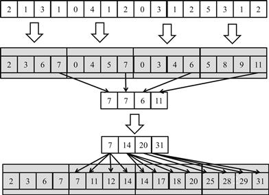
Figure 9.10 An example of a hierarchical scan.
For another example, the inputs in scan block 2 are 0, 3, 1, and 2. The kernel produces the scan result for this scan block (0, 3, 4, 6). To produce the final results for this scan block, the sum of all elements in both scan blocks 0 and 1 (2+1+3+1+0+4+1+2=14) should be added to every result element of scan block 2.
It is important to note that the last scan output element of each scan block gives the sum of all input elements of the scan block. These values are 7, 7, 6, and 11 in Figure 9.10. This brings us to the second step of the hierarchical scan algorithm in Figure 9.9, which gathers the last result elements from each scan block into an array and performs a scan on these output elements. This step is also illustrated in Figure 9.10, where the last scan output elements are all collected into a new array S. This can be done by changing the code at the end of the scan kernel so that the last thread of each block writes its result into an S array using its blockIdx.x as the index. A scan operation is then performed on S to produce output values 7, 14, 20, and 31. Note that each of these second-level scan output values are the accumulated sum from the beginning location X[0] to the end of each scan block. That is, the output value in S[0]=7 is the accumulated sum from X[0] to the end of scan block 0, which is X[3]. The output value in S[1]=14 is the accumulated sum from X[0] to the end of scan block 1, which is X[7].
Therefore, the output values in the S array give the scan results at “strategic” locations of the original scan problem. That is, in Figure 9.10, the output values in S[0], S[1], S[2], and S[3] give the final scan results for the original problem at positions X[3], X[7], X[11], and X[15]. These results can be used to bring the partial results in each scan block to their final values. This brings us to the last step of the hierarchical scan algorithm in Figure 9.9. The second-level scan output values are added to the values of their corresponding scan blocks.
For example, in Figure 9.10, the value of S[0] (7) will be added to Y[0], Y[1], Y[2], and Y[3] of thread block 1, which completes the results in these positions. The final results in these positions are 7, 11, 12, and 14. This is because S[0] contains the sum of the values of the original input X[0] through X[3]. These final results are 14, 17, 18, and 20. The value of S[1] (14) will be added to Y[8], Y[9], Y[10], and Y[11], which completes the results in these positions. The value of S[2] will be added to S[2] (20), which will be added to Y[12], Y[13], Y[14], and Y[15]. Finally, the value of S[3] is the sum of all elements of the original input, which is also the final result in Y[15].
Readers who are familiar with computer arithmetic algorithms should recognize that the hierarchical scan algorithm is quite similar to the carry look-ahead in hardware adders of modern processors.
We can implement the hierarchical scan with three kernels. The first kernel is largely the same as the kernel in Figure 9.7. We need to add one more parameter S, which has the dimension of InputSize/SECTION_SIZE. At the end of the kernel, we add a conditional statement for the last thread in the block to write the output value of the last XY element in the scan block to the blockIdx.x position of S:
__synchtrheads();
S[blockIdx.x] = XY[SECTION_SIZE – 1];
}
The second kernel is simply the same kernel as Figure 9.7, which takes S as input and writes S as output.
The third kernel takes the S and Y arrays as inputs and writes the output back into Y. The body of the kernel adds one of the S elements to all Y elements:
int i = blockIdx.x ∗ blockDim.x + threadIdx.x;
Y[i] += S[blockIdx.x];
We leave it as an exercise for readers to complete the details of each kernel and complete the host code.
9.6 Summary
In this chapter, we studied scan as an important parallel computation pattern. Scan is used to enable parallel allocation of resources parties of which the needs are not uniform. It converts seemingly sequential recursive computation into parallel computation, which helps to reduce sequential bottlenecks in many applications. We showed that a simple sequential scan algorithm performs only N additions for an input of N elements.
We first introduced a parallel scan algorithm that is conceptually simple but not work-efficient. As the data set size increases, the number of execution units needed for a parallel algorithm to break even with the simple sequential algorithm also increases. For an input of 1,024 elements, the parallel algorithm performs over nine times more additions than the sequential algorithm and requires at least nine times more executions to break even with the sequential algorithm. This makes the work-inefficient parallel algorithm inappropriate for power-limited environments such as mobile applications.
We then presented a work-efficient parallel scan algorithm that is conceptually more complicated. Using a reduction tree phase and a distribution tree phase, the algorithm performs only 2×N−3 additions no matter how large the input data sets are. Such work-efficient algorithms of which the number of operations grows linearly with the size of the input set are often also referred to as data-scalable algorithms. We also presented a hierarchical approach to extending the work-efficient parallel scan algorithm to handle the input sets of arbitrary sizes.
9.7 Exercises
9.1. Analyze the parallel scan kernel in Figure 9.2. Show that control divergence only occurs in the first warp of each block for stride values up to half of the warp size. That is, for warp size 32, control divergence will occur to iterations for stride values 1, 2, 4, 8, and 16.
9.2. For the work-efficient scan kernel, assume that we have 2,048 elements. How many add operations will be performed in both the reduction tree phase and the inverse reduction tree phase?
9.3. For the work-inefficient scan kernel based on reduction trees, assume that we have 2,048 elements. Which of the following gives the closest approximation on how many add operations will be performed?
9.4. Use the algorithm in Figure 9.3 to complete an exclusive scan kernel.
9.5. Complete the host code and all the three kernels for the hierarchical parallel scan algorithm in Figure 9.9.
9.6. Analyze the hierarchical parallel scan algorithm and show that it is work-efficient and the total number of additions is no more than 4×N − 3.
9.7. Consider the following array: [4 6 7 1 2 8 5 2]. Perform a parallel inclusive prefix scan on the array using the work-inefficient algorithm. Report the intermediate states of the array after each step.
9.8. Repeat Exercise 9.7 using the work-efficient algorithm.
9.9. Using the two-level hierarchical scan discussed in Section 9.5, what is the largest possible data set that can be handled if computing on a:
Reference
1. Harris, M. Parallel Prefix Sum with CUDA, Available at: 2007 <http://developer.download.nvidia.com/compute/cuda/1_1/Website/projects/scan/doc/scan.pdf>.