
Chapter 10
Parallel Patterns: Sparse Matrix–Vector Multiplication
An Introduction to Compaction and Regularization in Parallel Algorithms
Chapter Outline
10.1 Background
10.2 Parallel SpMV Using CSR
10.3 Padding and Transposition
10.4 Using Hybrid to Control Padding
10.5 Sorting and Partitioning for Regularization
10.6 Summary
10.7 Exercises
Our next parallel pattern is sparse matrix computation. In a sparse matrix, the vast majority of the elements are zeros. Storing and processing these zero elements are wasteful in terms of memory, time, and energy. Many important real-world problems involve sparse matrix computations that are highly parallel in nature. Due to the importance of these problems, several sparse matrix storage formats and their corresponding processing methods have been proposed and widely used in the field. All of them employ some type of compaction techniques to avoid storing or processing zero elements at the cost of introducing some level of irregularity into the data representation. Unfortunately, such irregularity can lead to underutilization of memory bandwidth, control flow divergence, and load imbalance in parallel computing. It is therefore important to strike a good balance between compaction and regularization. Some storage formats achieve a higher level of compaction at a high level of irregularity. Others achieve a more modest level of compaction while keeping the representation more regular. The parallel computation performance of their corresponding methods is known to be heavily dependent on the distribution of nonzero elements in the sparse matrices. Understanding the wealth of work in sparse matrix storage formats and their corresponding parallel algorithms gives a parallel programmer an important background for addressing compaction and regularization challenges in solving related problems.
10.1 Background
A sparse matrix is a matrix where the majority of the elements are zero. Sparse matrices arise in many science, engineering, and financial modeling problems. For example, as we saw in Chapter 7, matrices are often used to represent the coefficients in a linear system of equations. Each row of the matrix represents one equation of the linear system. In many science and engineering problems, there are a large number of variables and the equations involved are loosely coupled. That is, each equation only involves a small number of variables. This is illustrated in Figure 10.1, where variables x0 and x2 are involved in equation 0, none of the variables in equation 1, variables x1, x2, and x3 in equation 2, and finally variables x0 and x3 in equation 3.
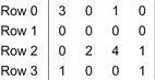
Figure 10.1 A simple sparse matrix example.
Sparse matrices are stored in a format that avoids storing zero elements. We will start with the compressed sparse row (CSR) storage format, which is illustrated in Figure 10.2. CSR stores only nonzero values in a 1D data storage, shown as data[] in Figure 10.2. Array data[] stores all the nonzero values in the sparse matrix in Figure 10.1. This is done by storing nonzero elements of row 0 (3 and 1) first, followed by nonzero elements of row 1 (none), followed by nonzero elements of row 2 (2, 4, 1), and then nonzero elements of row 3 (1, 1). The format compresses away all zero elements.

Figure 10.2 Example of CSR format.
With the compressed format, we need to put in two sets of markers to preserve the structure of the original sparse matrix. The first set of markers form a column index array, col_index[] in Figure 10.2, that gives the column index of every nonzero value in the original sparse matrix. Since we have squeezed away nonzero elements of each row, we need to use these markers to remember where the remaining elements were in the original row of the sparse matrix. For example, values 3 and 1 came from columns 0 and 2 of row 0 in the original sparse matrix. The col_index[0] and col_index[1] elements are assigned to store the column indices for these two elements. For another example, values 2, 4, and 1 came from columns 1, 2, and 3 in the original sparse matrix. Therefore, col_index[0], col_index[1], and col_index[2] store indices 1, 2, and 3.
The second set of markers give the starting location of every row in the compressed storage. This is because the size of each row becomes variable after zero elements are removed. It is no longer possible to use indexing based on the row size to find the starting location of each row in the compressed storage. In Figure 10.2, we show a row_ptr[] array of which the elements are the pointers or indices of the beginning locations of each row. That is, row_ptr[0] indicates that row 0 starts at location 0 of the data[] array, row_ptr[1] indicates that row 1 starts at location 2, etc. Note that row_ptr[1] and row_ptr[2] are both 2. This means that none of the elements of the row 1 was stored in the compressed format. This makes sense since row 1 in Figure 10.1 consists entirely of zero values. Note also that row_ptr[5] stores the starting location of a nonexisting row 4. This is for convenience, as some algorithms need to use the starting location of the next row to delineate the end of the current row. This extra marker gives a convenient way to locate the ending location of row 3.
As we discussed in Chapter 7, matrices are often used in solving a linear system of N equations of N variables in the form of A×X+Y=0, where A is an N×N matrix, X is a vector of N variables, and Y is a vector of N constant values. The objective is to solve for the X variable values that will satisfy all the questions. An intuitive approach is to Invert the matrix so that X=A−1×(−Y). This can be done through methods such as Gaussian elimination for moderate-size arrays. While it is theoretically possible to solve equations represented in sparse matrices, the sheer size and the number of zero elements of many sparse linear systems of equations can simply overwhelm this intuitive approach.
Instead, sparse linear systems can often be better solved with an iterative approach. When the sparse matrix A is positive-definite (i.e., xTAx>0 for all nonzero vectors x in Rn), one can use conjugate gradient methods to iteratively solve the corresponding linear system with guaranteed convergence to a solution [Hest1952]. This is done by guessing a solution X, perform A×X+Y, and see if the result is close to a 0 vector. If not, we can use a gradient vector formula to refine the guessed X and perform another iteration of A×X+Y using the refined X. The most time-consuming part of such an iterative approach is in the evaluation of A×X+Y, which is a sparse matrix–vector multiplication and accumulation. Figure 10.3 shows a small example of matrix-vector multiplication, where A is a sparse matrix. The dark squares in A represent non-zero elements. In contrast, both X and Y are typically dense vectors. That is, most of the elements of X and Y hold non-zero values. Due to its importance, standardized library function interfaces have been created to perform this operation under the name SpMV (sparse matrix–vector multiplication). We will use SpMV to illustrate the important trade-offs between different storage formats of sparse computation.
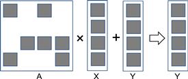
Figure 10.3 A small example of matrix–vector multiplication and accumulation.
A sequential implementation of SpMV based on CSR is quite straightforward, which is shown in Figure 10.4. We assume that the code has access to (1) num_rows, a function argument that specifies the number of rows in the sparse matrix, and (2) a floating-point data[] array and two integer row_ptr[] and x[] arrays as in Figure 10.3. There are only seven lines of code. Line 1 is a loop that iterates through all rows of the matrix, with each iteration calculating a dot product of the current row and the vector x.
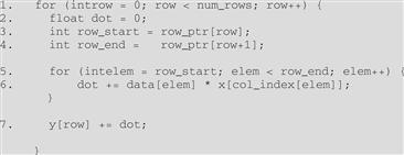
Figure 10.4 A sequential loop that implements SpMV.
In each row, line 2 first initializes the dot product to zero. It then sets up the range of data[] array elements that belong to the current row. The starting and ending locations can be loaded from the row_ptr[] array. Figure 10.5 illustrates this for the small sparse matrix in Figure 10.1. For row=0, row_ptr[row] is 0 and row_ptr[row+1] is 2. Note that the two elements from row 0 reside in data[0] and data[1]. That is, row_ptr[row] gives the starting position of the current row and row_ptr[row+1] gives the starting position of the next row, which is one after the ending position of the current row. This is reflected in the loop in line 5, where the loop index iterates from the position given by row_ptr[row] to row_ptr[row+1]−1.
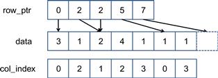
Figure 10.5 SpMV loop operating on the sparse matrix in Figure 10.1.
The loop body in line 6 calculates the dot product for the current row. For each element, it uses the loop index elem to access the matrix element in data[elem]. It also uses elem to retrieve the column index for the element from col_index[elem]. This column index is then used to access the appropriate x element for multiplication. For example, the element in data[0] and data[1] are from column 0 (col_index[0]=0) and column 2 (col_index[1]=2). So the inner loop will perform the dot product for row 0 as data[0]∗x[0]+data[1]∗x[2]. Readers are encouraged to work out the dot product for other rows as an exercise.
CSR completely removes all zero elements from the storage. It does incur an overhead by introducing the col_index and row_ptr arrays. In our small example, where the number of zero elements are not much more than the non-zero elements, the overhead is slightly more than the space needed for the nonzero elements.
It should be obvious that any SpMV code will reflect the storage format assumed. Therefore, we will add the storage format to the name of a code to clarify the combination used. We will refer to the SpMV code in Figure 10.4 as sequential SpMV/CSR. With a good understanding of sequential SpMV/CSR, we are now ready to discuss parallel sparse computation.
10.2 Parallel SpMV Using CSR
Note that the dot product calculation for each row of the sparse matrix is independent of those of other rows. This is reflected in the fact that all iterations of the outer loop (line 1) in Figure 10.4 are logically independent of each other. We can easily convert this sequential SpMV/CSR into a parallel CUDA kernel by assigning each iteration of the outer loop to a thread, which is illustrated in Figure 10.6, where thread 0 calculates the dot product for row 0, thread 1 for row 1, and so on.
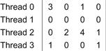
Figure 10.6 Example of mapping threads to rows in parallel SpMV/CSR.
In a real sparse matrix computation, there are usually thousands to millions of rows, each of which contain tens to hundreds of nonzero elements. This makes the mapping shown in Figure 10.6 seem very appropriate: there are many threads and each thread has a substantial amount of work. We show a parallel SpMV/CSR in Figure 10.7.
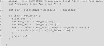
Figure 10.7 A parallel SpMV/CSR kernel.
It should be clear that the kernel looks almost identical to the sequential SpMV/CSR loop. The loop construct has been removed since it is replaced by the thread grid. All the other changes are very similar to the case of the vector addition kernel in Chapter 3. In line 2, the row index is calculated as the familiar expression blockIdx.x ∗ blockDim.x + threadIdx.x. Also, due to the need to handle an arbitrary number of rows, line 3 checks if the row index of a thread exceeds the number of rows. This handles the situation where the number of rows is not a multiple of thread block size.
While the parallel SpMV/CSR kernel is quite simple, it has two major shortcomings. First the kernel does not make coalesced memory accesses. If readers examine Figure 10.5, it should be obvious that adjacent threads will be making simultaneous nonadjacent memory accesses. In our small example, threads 0, 1, 2, and 3 will access data[0], none, data[2], and data[5] in the first iteration of their dot product loop. They will then access data[1], none, data[3], and data[6] in the second iterations, and so on. It is obvious that these simultaneous accesses made by adjacent threads are not to adjacent locations. As a result, the parallel SpMV/CSR kernel does not make efficient use of memory bandwidth.
The second shortcoming of the SpMV/CSR kernel is that it can potentially have significant control flow divergence in all warps. The number of iterations taken by a thread in the dot product loop depends on the number of nonzero elements in the row assigned to the thread. Since the distribution of nonzero elements among rows can be random, adjacent rows can have a very different number of nonzero elements. As a result, there can be widespread control flow divergence in most or even all warps.
It should be clear that both the execution efficiency and memory bandwidth efficiency of the parallel SpMV kernel depends on the distribution of the input data matrix. This is quite different from most of the kernels we have presented so far. However, such data-dependent performance behavior is quite common in real-world applications. This is one of the reasons why parallel SpMV is such an important parallel pattern—it is simple and yet it illustrates an important behavior in many complex parallel applications. We will discuss the important techniques in the next sections to address the two shortcomings of the parallel SpMV/CSR kernel.
10.3 Padding and Transposition
The problems of noncoalesced memory accesses and control divergence can be addressed with data padding and transposition of matrix layout. The ideas were used in the ELL storage format, the name of which came from the sparse matrix package ELLPACK. A simple way to understand the ELL format is to start with the CSR format, as illustrated in Figure 10.8.
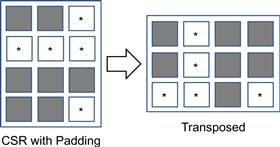
Figure 10.8 ELL storage format.
From a CSR representation, we first determine the rows with the maximal number of nonzero elements. We then add dummy (zero) elements to all other rows after the nonzero elements to make them the same length as the maximal rows. This makes the matrix a rectangular matrix. For our small sparse matrix example, we determine that row 2 has the maximal number of elements. We then add one zero element to row 0, three zero elements to row 1, and one zero element to row 3 to make all them the same length. These additional zero elements are shown as squares with an ∗ in Figure 10.8. Now the matrix has become a rectangular matrix. Note that the col_index array also needs to be padded the same way to preserve their correspondence to the data values.
We can now lay out the padded matrix in column-major order. That is, we will place all elements of column 0 in consecutive locations, followed by all elements of column 1, and so on. This is equivalent to transposing the rectangular matrix and layout out the matrix in the row-major order of C. In terms of our small example, after the transposition, data[0] through data[3] now contain 3, ∗, 2, 1, the zero elements of all rows. This is illustrated in the bottom portion of Figure 10.9. col_index[0] through col_index[3] contain the first elements of all rows. Note that we no longer need the row_ptr since the beginning of row i is now simply data[i]. With the padded elements, it is also very easy to move from the current element of row i to the next element by simply adding the number of rows to the index. For example, the zero element of row 2 is in data[2] and the next element is in data[2+4]=data[6], where 4 is the number of rows in our small example.
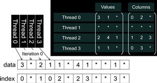
Figure 10.9 More details of our small example in ELL.
Using the ELL format, we show a parallel SpMV/ELL kernel in Figure 10.10. The kernel receives a slightly different argument. It no longer needs the row_ptr. Instead, it needs an argument num_elem to know the number of elements in each row after padding.
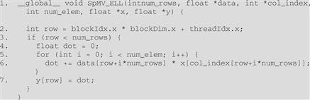
Figure 10.10 A parallel SpMV/ELL kernel.
A first observation is that the SpMV/ELL kernel code is simpler than SpMV/CSR. With padding, all rows are now of the same length. In the dot product loop in line 5, all threads can simply loop through the number of elements given by num_elem. As a result, there is no longer control flow divergence in warps: all threads now iterate exactly the same number of times in the dot product loop. In the case where a dummy element is used in the multiplication, since its value is zero, it will not affect the final result.
A second observation is that in the dot product loop body, each thread accesses its zero element in data[row] and then access its i element in data[row+i∗num_rows]. As we have seen in Figure 10.10, all adjacent threads are now accessing adjacent memory locations, enabling memory coalescing and thus making more efficient use of memory bandwidth.
By eliminating control flow divergence and enabling memory coalescing, SpMV/ELL should run faster than SpMV/CSR. Furthermore, SpMV/ELL is simpler. This seems to make SpMV/ELL an all-winning approach. However, it is not quite so. Unfortunately, it does have its potential downside. In situations where one or a small number of rows have an exceedingly large number of nonzero elements, the ELL format will result in an excessive number of padded elements. These padded elements will take up storage, need to be fetched, and take part in calculations even though they do not contribute to the final result. With enough padded elements, an SpMV/ELL kernel can actually run more slowly than an SpMV/CSR kernel. This calls for a method to control the number of padded elements in an ELL representation.
10.4 Using Hybrid to Control Padding
The root of the problem with excessive padding in ELL is that one or a small number of rows have an exceedingly large number of nonzero elements. If we have a mechanism to “take away” some elements from these rows, we can reduce the number of padded elements in ELL. The coordinate (COO) format provides such a venue.
The COO format is illustrated in Figure 10.11, where each nonzero element is stored with both its column index and row index. We have both col_index and row_index arrays to accompany the data array. For example A[0,0] of our small example is now stored with both its column index (0 in col_index[0]) and its row index (0 in row_index[0]). With COO format, one can look at any element in the storage and know where the nonzero element came from in the original sparse matrix. Like the ELL format, there is no need for row_ptr since each element self-identifies its column and row index.
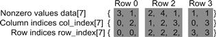
Figure 10.11 Example of COO format.
While the COO format does come with the cost of additional storage for the row_index array, it also comes with the additional benefit of flexibility. We can arbitrarily reorder the elements in a COO format without losing any information as long as we reorder the data, col_index, and row_index the same way. This is illustrated using our small example in Figure 10.12.
![]()
Figure 10.12 Reordering COO format.
In Figure 10.12, we have reordered the elements of data, col_index, and row_index. Now data[0] actually contains an element from row 0 and column 3 of the small sparse matrix. Because we have also shifted the row index and column index values along with the data value, we can correctly identify this element in the original sparse matrix. Readers may ask why we would want to reorder these elements. Such reordering would disturb the locality and sequential patterns that are important for efficient use of memory bandwidth.
The answer lies in an important use case for the COO format. It can be used to curb the length of the CSR or ELL format. First, we will make an important observation. In the COO format, we can process the elements in any order we want. For each element in data[i], we can simply perform a y[row_index[i]] += data[i] ∗ x[col_index[i]] operation. If we make sure somehow we perform this operation for all elements of data, we will calculate the correct final answer.
More importantly, we can take away some of the elements from the rows with an exceedingly large number of nonzero elements and place them into a separate COO format. We can use either CSR or ELL to perform SpMV on the remaining elements. With excess elements removed from the extra-long rows, the number of padded elements for other rows can be significantly reduced. We can then use a SpMV/COO to finish the job. This approach of employing two formats to collaboratively complete a computation is often referred to as a hybrid method.
Let’s illustrate a hybrid ELL and COO method for SpMV using our small sparse matrix, as shown in Figure 10.13. We see that row 2 has the most number of nonzero elements. We remove the last nonzero element of row 2 from the ELL representation and move it into a separate COO representation. By removing the last element of row 2, we reduce the maximal number of nonzero elements among all rows in the small sparse matrix from 3 to 2. As shown in Figure 10.13, we reduce the number of padded elements from 5 to 2. More importantly, all threads now only need to take two iterations rather than three. This can give a 50% acceleration to the parallel execution of the SpMV/ELL kernel.
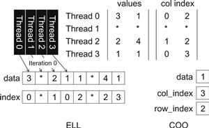
Figure 10.13 Our small example in ELL and COO hybrid.
A typical way of using an ELL-COO hybrid method is for the host to convert the format from something like a CSR format into ELL. During the conversion, the host removes some nonzero elements from the rows with an exceedingly large number of nonzero elements. The host places these elements into a COO representation. The host then transfers the ELL representation of the data to a device. When the device completes the SpMV/ELL kernel, it transfers the y values back to the host. These values are missing the contributions from the elements in the COO representation. The host performs a sequential SpMV/COO on the COO elements and finishes their contributions to the y element values.
The user may question whether the additional work done by the host to separate COO elements from an ELL format could incur too much overhead. The answer is it depends. In situations where a sparse matrix is only used in one SpMV calculation, this extra work can indeed incur significant overhead. However, in many real-world applications, the SpMV is performed on the same sparse kernel repeated in an iterative solver. In each iteration of the solver, the x and y vectors vary but the sparse matrix remains the same since its elements correspond to the coefficients of the linear system of equations being solved and these coefficients do not change from iteration to iteration. So, the work done to produce both the ELL and COO representation can be amortized across many iterations. We will come back to this point in the next section.
In our small example, the device finishes the SpMV/ELL kernel on the ELL portion of the data. The y values are then transferred back to the host. The host then adds the contribution of the COO element with the operation y[2] += data[0] ∗ x[col_index[0]] = 1∗x[3]. Note that there are in general multiple nonzero elements in the COO format. So, we expect that the host code to be a loop as shown in Figure 10.14.
![]()
Figure 10.14 A sequential loop that implements SpMV/COO.
The loop is extremely simple. It iterates through all the data elements and performs the multiply and accumulate operations on the appropriate x and y elements using the accompanying col_index and row_index elements. We will not present a parallel SpMV/COO kernel. It can be easily constructed using each thread to process a portion of the data elements and use an atomic operation to accumulate the results into y elements. This is because the threads are no longer mapped to a particular row. In fact, many rows will likely be missing from the COO representation; only the rows that have an exceedingly large number of nonzero elements will have elements in the COO representation. Therefore, it is better just to have each thread to take a portion of the data element and use an atomic operation to make sure that none of the threads will trample the contribution of other threads.
The hybrid SpMV/ELL-COO method is a good illustration of productive use of both CPUs and GPUs in a heterogeneous computing system. The CPU can perform SpMV/COO fast using its large cache memory. The GPU can perform SpMV/ELL fast using its coalesced memory accesses and large number of hardware execution units. The removal of some elements from the ELL format is a form of regularization technique: it reduces the disparity between long and short rows and makes the workload of all threads more uniform. Such improved uniformity results in benefits such as less control divergence in a SpMV/CSR kernel or less padding in a SpMV/ELL kernel.
10.5 Sorting and Partitioning for Regularization
While COO helps to regulate the amount of padding in an ELL representation, we can further reduce the padding overhead by sorting and partitioning the rows of a sparse matrix. The idea is to sort the rows according to their length, say from the longest to the shortest. This is illustrated with our small sparse matrix in Figure 10.15. Since the sorted matrix looks largely like a triangular matrix, the format is often referred to as jagged diagonal storage (JDS). As we sort the rows, we typically maintain an additional jds_row_index array that preserves the original index of the row. For CSR, this is similar to the row_ptr array in that there is one element per row. Whenever we exchange two rows in the sorting process, we also exchange the corresponding elements of the jds_row_index array. This way, we can always keep track of the original position of all rows.
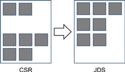
Figure 10.15 Sorting rows according to their length.
Once a sparse matrix is in JDS format, we can partition the matrix into sections of rows. Since the rows have been sorted, all rows in a section will likely have a more or less uniform number of nonzero elements. In Figure 10.15, we can divide the small matrix into three sections: the first section consists of the one row that has three elements, the second section consists of the two rows with two elements each, and the third section consists of one row without any element. We can then generate ELL representation for each section. Within each section, we only need to pad the rows to match the row with the maximal number of elements in that section. This would reduce the number of padded elements. In our example, we do not even need to pad within any of the three sections. We can then transpose each section independently and launch a separate kernel on each section. In fact, we do not even need to launch a kernel for the section of rows with no nonzero elements.
Figure 10.16 shows a JDS-ELL representation of our small sparse matrix. It assumed the same sorting and partitioning results shown in Figure 10.15. Out of the three sections, the first section has only one row so the transposed layout is the same as the original. The second section is a 2 × 2 matrix and has been transposed. The third section consists of row 1, which does not have any nonzero element. This is reflected in the fact that its starting location and the next section’s starting position are identical.
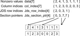
Figure 10.16 JDS format and sectioned ELL.
We will not show a SpMV/JDS kernel. The reason is that we would be just using either an SpMV/CSR kernel on each section of the CSR, or a SpMV/ELL kernel on each section of the ELL after padding. The host code required to create a JDS representation and to launch SpMV kernels on each section of the JDS representation is left as an exercise.
Note that we want each section to have a large number of rows so that its kernel launch will be worthwhile. In the extreme cases where a very small number of rows have an extremely large number of nonzero elements, we can still use the COO hybrid with JDS to allow us to have more rows in each section.
Once again readers should ask whether sorting rows will result into incorrect solutions to the linear system of equations. Recall that we can freely reorder equations of a linear system without changing the solution. As long as we reorder the y elements along with the rows, we are effectively reordering the equations. Therefore, we will end up with the correct solution. The only extra step is to reorder the final solution back to the original order using the jds_row_index array.
The other question is whether sorting will incur significant overhead. The answer is similar to what we saw in the hybrid method. As long as the SpMV/JDS kernel is used in an iterative solver, one can afford to perform such sorting as well as the reordering of the final solution x elements and amortize the cost among many iterations of the solver.
In more recent devices, the memory coalescing hardware has relaxed the address alignment requirement. This allows one to simply transpose a JDS-CSR representation. Note that we do need to adjust the jds_section_ptr array after transposition. This further eliminates the need to pad rows in each section. As memory bandwidth becomes increasingly the limiting factor of performance, eliminating the need to store and fetch padded elements can be a significant advantage. Indeed, we have observed that while sectioned JDS-ELL tends to give the best performance on older CUDA devices, transposed JDS-CSR tends to give the best performance on Fermi and Kepler.
We would like to make an additional remark on the performance of sparse matrix computation as compared to dense matrix computation. In general, the FLOPS rating achieved by either CPUs or GPUs are much lower for sparse matrix computation than for dense matrix computation. This is especially true for SpMV, where there is no data reuse in the sparse matrix. The CGMA value (see Chapter 5) is essentially 1, limiting the achievable FLOPS rate to a small fraction of the peak performance. The various formats are important for both CPUs and GPUs since both are limited by memory bandwidth when performing SpMV. Many folks have been surprised by the low FLOPS rating of this type of computation on both CPUs and GPUs in the past. After reading this chapter, one should no longer be surprised.
10.6 Summary
In this chapter, we presented sparse matrix computation as an important parallel pattern. Sparse matrices are important in many real-world applications that involve modeling complex phenomenon. Furthermore, sparse matrix computation is a simple example of data-dependent performance behavior of many large real-world applications. Due to the large amount of zero elements, compaction techniques are used to reduce the amount of storage, memory accesses, and computation performed on these zero elements. Unlike most other kernels presented in this book so far, the SpMV kernels are sensitive to the distribution of nonzero elements in the sparse matrices. Not only can the performance of each kernel vary significantly across matrices, their relative merit can also change significantly. Using this pattern, we introduce the concept of regularization using hybrid methods and sorting/partitioning. These regularization methods are used in many real-world applications. Interestingly, some of the regularization techniques reintroduce zero elements into the compacted representations. We use hybrid methods to mitigate the pathological cases where we could introduce too many zero elements. Readers are referred to [Bell2009] and encouraged to experiment with different sparse data sets to gain more insight into the data-dependent performance behavior of the various SpMV kernels presented in this chapter.
10.7 Exercises
10.1. Complete the host code to produce the hybrid ELL-COO format, launch the ELL kernel on the device, and complete the contributions of the COO elements.
10.2. Complete the host code for producing JDS-ELL and launch one kernel for each section of the representation.
10.3. Consider the following sparse matrix:
1 0 7 0
0 0 8 0
0 4 3 0
2 0 0 1
Represent it in each of the following formats: (a) COO, (b) CSR, and (c) ELL.
10.4. Given a sparse matrix of integers with m rows, n columns, and z nonzeros, how many integers are needed to represent the matrix in (a) COO, (b) CSR, and (c) ELL. If the information provided is not enough, indicate what information is missing.
References
1. Hestenes M, Stiefel E. Methods of conjugate gradients for solving linear systems. Journal of Research of the National Bureau of Standards. 1952;49.
2. Bell, N., & Garland, M. Implementing sparse matrix-vector multiplication on throughput-oriented processors, Proceedings of the ACM Conference on High-Performance Computing Networking Storage and Analysis (SC’09), 2009.