
Chapter 19
Programming a Heterogeneous Computing Cluster
Chapter Outline
19.1 Background
19.2 A Running Example
19.3 MPI Basics
19.4 MPI Point-to-Point Communication Types
19.5 Overlapping Computation and Communication
19.6 MPI Collective Communication
19.7 Summary
19.8 Exercises
So far we have focused on programming a heterogeneous computing system with one host and one device. In high-performance computing (HPC), many applications require the aggregate computing power of a cluster of computing nodes. Many of the HPC clusters today have one or more hosts and one or more devices in each node. Historically, these clusters have been programmed predominately with the Message Passing Interface (MPI). In this chapter, we will present an introduction to joint MPI/CUDA programming. Readers should be able to easily extend the material to joint MPI/OpenCL, MPI/OpenACC, and so on. We will only present the key MPI concepts that programmers need to understand to scale their heterogeneous applications to multiple nodes in a cluster environment. In particular, we will focus on domain partitioning, point-to-point communication, and collective communication in the context of scaling a CUDA kernel into multiple nodes.
19.1 Background
While there was practically no top supercomputer using GPUs before 2009, the need for better energy efficiency has led to fast adoption of GPUs in recent years. Many of the top supercomputers in the world today use both CPUs and GPUs in each node. The effectiveness of this approach is validated by their high rankings in the Green 500 list, which reflects their high energy efficiency.
The dominating programming interface for computing clusters today is MPI [Gropp1999], which is a set of API functions for communication between processes running in a computing cluster. MPI assumes a distributed memory model where processes exchange information by sending messages to each other. When an application uses API communication functions, it does not need to deal with the details of the interconnect network. The MPI implementation allows the processes to address each other using logical numbers, much the same way as using phone numbers in a telephone system: telephone users can dial each other using phone numbers without knowing exactly where the called person is and how the call is routed.
In a typical MPI application, data and work are partitioned among processes. As shown in Figure 19.1, each node can contain one or more processes, shown as clouds within nodes. As these processes progress, they may need data from each other. This need is satisfied by sending and receiving messages. In some cases, the processes also need to synchronize with each other and generate collective results when collaborating on a large task. This is done with collective communication API functions.
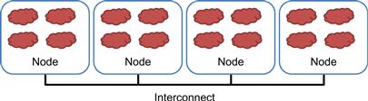
Figure 19.1 Programmer’s view of MPI processes.
19.2 A Running Example
We will use a 3D stencil computation as a running example. We assume that the computation calculates heat transfer based on a finite difference method for solving a partial differential equation that describes the physical laws of heat transfer. In each step, the value of a grid point is calculated as a weighted sum of neighbors (north, east, south, west, up, down) and its own value from the previous time step. To achieve high numerical stability, multiple indirect neighbors in each direction are also used in the computation of a grid point. This is referred to as a higher-order stencil computation. For the purpose of this chapter, we assume that four points in each direction will be used. As shown in Figure 19.2, there are a total of 24 neighbor points for calculating the next step value of a grid point. As shown in Figure 19.2, each point in the grid has an x, y, and z coordinate. For a grid point where the coordinate value is x=i, y=j, and z=k, or (i,j,k), its 24 neighbors are (i−4,j,k), (i−3,j,k), (i−2,j,k), (i−1,j,k), (i+1,j,k), (i+2,j,k), (i+3,j,k), (i+4,j,k), (i,j−4,k), (i,j−3,k), (i,j−2,k), (i,j−1,k), (i,j+1,k), (i,j+2,k), (i,j+3,k), (i,j+4,k), (i,j,k−4), (i,j,k−3), (i,j,k−2), (i,j,k−1), (i,j,k+1), (i,j,k+2), (i,j,k+3), and (i,j,k+4). Since the next data value of each grid point is calculated based on the current data values of 25 points (24 neighbors and itself), the type of computation is often called 25-stencil computation.

Figure 19.2 A 25-stencil computation example, where the neighbors are in the x, y, and z directions.
We assume that the system is modeled as a structured grid, where spacing between grid points is constant within each direction. This allows us to use a 3D array where each element stores the state of a grid point. The physical distance between adjacent elements in each dimension can be represented by a spacing variable. Figure 19.3 illustrates a 3D array that represents a rectangular ventilation duct, with x and y dimensions as the cross-sections of the duct and the z dimension the direction of the heat flow along the duct.
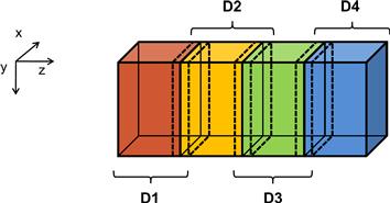
Figure 19.3 3D grid array for modeling the heat transfer in a duct.
We assume that the data is laid out in the memory space and that x is the lowest dimension, y is the next, and z is the highest. That is, all elements with y=0 and z=0 will be placed in consecutive memory locations according to their x coordinate. Figure 19.4 shows a small example of the grid data layout. This small example has only 16 data elements in the grid: two elements in the x dimension, two in the y dimension, and four in the z dimension. Both x elements with y=0 and z=0 are placed in memory first. They are followed by all elements with y=1 and z=0. The next group will be elements with y=0 and z=1.
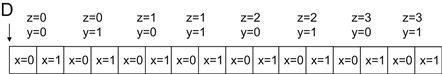
Figure 19.4 A small example of memory layout for the 3D grid.
When one uses a cluster, it is common to divide the input data into several partitions, called domain partitions, and assign each partition to a node in the cluster. In Figure 19.3, we show that the 3D array is divided into four domain partitions: D1, D2, D3, and D4. Each of the partitions will be assigned to an MPI compute process.
The domain partition can be further illustrated with Figure 19.4. The first section, or slice, of four elements (z=0) in Figure 19.4 is in the first partition, the second section (z=1) the second partition, the third section (z=2) the third partition, and the fourth section (z=3) the fourth partition. This is obviously a toy example. In a real application, there are typically hundreds or even thousands of elements in each dimension. For the rest of this chapter, it is useful to remember that all elements in a z slice are in consecutive memory locations.
19.3 MPI Basics
Like CUDA, MPI programs are based on the SPMD (single program, multiple data) parallel execution model. All MPI processes execute the same program. The MPI system provides a set of API functions to establish communication systems that allow the processes to communicate with each other. Figure 19.5 shows five essential API functions that set up and tear down communication systems for an MPI application. Figure 19.6 shows a simple MPI program that uses these API functions. A user needs to supply the executable file of the program to the mpirun command or the mpiexec command in a cluster.
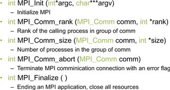
Figure 19.5 Five basic MPI–API functions for establishing and closing a communication system.
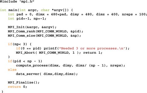
Figure 19.6 A simple MPI main program.
Each process starts by initializing the MPI runtime with a MPI_Init() call. This initializes the communication system for all the processes running the application. Once the MPI runtime is initialized, each process calls two functions to prepare for communication. The first function is MPI_Comm_rank(), which returns a unique number to calling each process, called an MPI rank or process ID. The numbers received by the processes vary from 0 to the number of processes minus 1. MPI rank for a process is equivalent to the expression blockIdx.x∗blockDim.x+threadIdx.x for a CUDA thread. It uniquely identifies the process in a communication, similar to the phone number in a telephone system.
The MPI_Comm_rank() takes two parameters. The first one is an MPI built-in type MPI_Comm that specifies the scope of the request. Values of the MPI_Comm are commonly referred to as a communicator. MPI_Comm and other MPI built-in types are defined in a mpi.h header file that should be included in all C program files that use MPI. This is similar to the cuda.h header file for CUDA programs. An MPI application can create one or more intracommunicators. Members of each intracommunicator are MPI processes. MPI_Comm_rank() assigns a unique ID to each process in an intracommunicator. In Figure 19.6, the parameter value passed is MPI_COMM_WORLD, which means that the intracommunicator includes all MPI processes running the application.
The second parameter to the MPI_Comm_rank() function is a pointer to an integer variable into which the function will deposit the returned rank value. In Figure 19.6, a variable pid is declared for this purpose. After the MPI_Comm_rank() returns, the pid variable will contain the unique ID for the calling process.
The second API function is MPI_Comm_size(), which returns the total number of MPI processes running in the intracommunicator. The MPI_Comm_size() function takes two parameters. The first one is an MPI built-in type MPI_Comm that gives the scope of the request. In Figure 19.6, the scope is MPI_COMM_WORLD. Since we use MPI_COMM_WORLD, the returned value is the number of MPI processes running the application. This is requested by a user when the application is submitted using the mpirun command or the mpiexec command. However, the user may not have requested a sufficient number of processes. Also, the system may or may not be able to create all the processes requested. Therefore, it is good practice for an MPI application program to check the actual number of processes running.
The second parameter is a pointer to an integer variable into which the MPI_Comm_size() function will deposit the return value. In Figure 19.6, a variable np is declared for this purpose. After the function returns, the variable np contains the number of MPI processes running the application. In Figure 19.6, we assume that the application requires at least three MPI processes. Therefore, it checks if the number of processes is at least three. If not, it calls the MPI_Comm_abort() function to terminate the communication connections and return with an error flag value of 1.
Figure 19.6 also shows a common pattern for reporting errors or other chores. There are multiple MPI processes but we need to report the error only once. The application code designates the process with pid=0 to do the reporting.
As shown in Figure 19.5, the MPI_Comm_abort() function takes two parameters. The first is the scope of the request. In Figure 19.6, the scope is all MPI processes running the application. The second parameter is a code for the type of error that caused the abort. Any number other than 0 indicates that an error has happened.
If the number of processes satisfies the requirement, the application program goes on to perform the calculation. In Figure 19.6, the application uses np-1 processes (pid from 0 to np-2) to perform the calculation and one process (the last one of which the pid is np-1) to perform an input/output (I/O) service for the other processes. We will refer to the process that performs the I/O services as the data server and the processes that perform the calculation as compute processes. In Figure 19.6, if the pid of a process is within the range from 0 to np-2, it is a compute process and calls the compute_process() function. If the process pid is np-1, it is the data server and calls the data_server() function.
After the application completes its computation, it notifies the MPI runtime with a call to the MPI_Finalize(), which frees all MPI communication resources allocated to the application. The application can then exit with a return value 0, which indicates that no error occurred.
19.4 MPI Point-to-Point Communication Types
MPI supports two major types of communication. The first is the point-to-point type, which involves one source process and one destination process. The source process calls the MPI_Send() function and the destination process calls the MPI_Recv() function. This is analogous to a caller dialing a call and a receiver answering a call in a telephone system.
Figure 19.7 shows the syntax for using the MPI_Send() function. The first parameter is a pointer to the starting location of the memory area where the data to be sent can be found. The second parameter is an integer that gives that number of data elements to be sent. The third parameter is of an MPI built-in type MPI_Datatype. It specifies the type of each data element being sent. The MPI_Datatype is defined in mpi.h and includes MPI_DOUBLE (double precision, floating point), MPI_FLOAT (single precision, floating point), MPI_INT (integer), and MPI_CHAR (character). The exact sizes of these types depend on the size of the corresponding C types in the host processor. See the MPI programming guild for more sophisticated uses of MPI types [Gropp 1999].
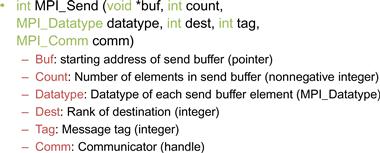
Figure 19.7 Syntax for the MPI_Send() function.
The fourth parameter for MPI_Send is an integer that gives the MPI rank of the destination process. The fifth parameter gives a tag that can be used to classify the messages sent by the same process. The sixth parameter is a communicator that selects the processes to be considered in the communication.
Figure 19.8 shows the syntax for using the MPI_Recv() function. The first parameter is a pointer to the area in memory where the received data should be deposited. The second parameter is an integer that gives the maximal number of elements that the MPI_Recv() function is allowed to receive. The third parameter is an MPI_Datatype that specifies the type (size) of each element to be received. The fourth parameter is an integer that gives the process ID of the source of the message.
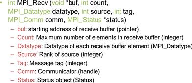
Figure 19.8 Syntax for the MPI_Recv() function.
The fifth parameter is an integer that specifies the particular tag value expected by the destination process. If the destination process does not want to be limited to a particular tag value, it can use MPI_ANY_TAG, which means that the receiver is willing to accept messages of any tag value from the source.
We will first use the data server to illustrate the use of point-to-point communication. In a real application, the data server process would typically perform data input and output operations for the compute processes. However, input and output have too much system-dependent complexity. Since I/O is not the focus of our discussion, we will avoid the complexity of I/O operations in a cluster environment. That is, instead of reading data from a file system, we will just have the data server initialize the data with random numbers and distribute the data to the compute processes. The first part of the data server code is shown in Figure 19.9.
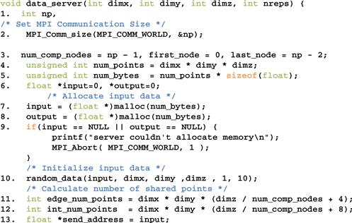
Figure 19.9 Data server process code (part 1).
The data server function takes four parameters. The first three parameters specify the size of the 3D grid: number of elements in the x dimension is dimx, the number of elements in the y dimension is dimy, and the number of elements in the z dimension is dimz. The fourth parameter specifies the number of iterations that need to be done for all the data points in the grid.
In Figure 19.9, line 1 declares variable np that will contain the number of processes running the application. Line 2 calls MPI_Comm_size(), which will deposit the information into np. Line 3 declares and initializes several helper variables. The variable num_comp_procs contains the number of compute processes. Since we are reserving one process as the data server, there are np-1 compute processes. The variable first_proc gives the process ID of the first compute process, which is 0. The variable last_proc gives the process ID of the last compute process, which is np-2. That is, line 3 designates the first np-1 processes, 0 through np-2, as compute processes. This reflects the design decision and the process with the largest rank serves as the data server. This decision will also be reflected in the compute process code.
Line 4 declares and initializes the num_points variable that gives the total number of grid data points to be processed, which is simply the product of the number of elements in each dimension, or dimx ∗ dimy ∗ dimz. Line 5 declares and initializes the num_bytes variable that gives the total number of bytes needed to store all the grid data points. Since each grid data point is a float, this value is num_points ∗ sizeof(float).
Line 6 declares two pointer variables: input and output. These two pointers will point to the input data buffer and the output data buffer, respectively. Lines 7 and 8 allocate memory for the input and output buffers and assign their addresses to their respective pointers. Line 9 checks if the memory allocations were successful. If either of the memory allocations fail, the corresponding pointer will receive a NULL pointer from the malloc() function. In this case, the code aborts the application and reports an error.
Lines 11 and 12 calculate the number of grid point array elements that should be sent to each compute process. As shown in Figure 19.3, there are two types of compute processes. The first process (process 0) and the last process (process 3) compute an “edge” partition that has neighbors only on one side. Partition 0 assigned to the first process has a neighbor only on the right side (partition 1). Partition 3 assigned to the last process has a neighbor only on the left side (partition 2). We call the compute processes that compute edge partitions the edge processes.
Each of the rest of the processes computes an internal partition that has neighbors on both sizes. For example, the second process (process 1) computes a partition (partition 1) that has a left neighbor (partition 0) and a right neighbor (partition 2). We call the processes that compute internal partitions internal processes.
Recall that each calculation step for a grid point needs the values of its immediate neighbors from the previous step. This creates a need for halo cells for grid points at the left and right boundaries of a partition, shown as slices defined by dotted lines at the edge of each partition in Figure 19.3. Note that these halo cells are similar to those in the convolution pattern presented in Chapter 8. Therefore, each process also needs to receive one slice of halo cells that contains all neighbors for the boundary grid points of its partition. For example, in Figure 19.3, partition D2 needs a halo slice from D1 and a halo slice from D3. Note that a halo slice for D2 is a boundary slice for D1 or D3.
Recall that the total number of grid points is dimx∗dimy∗dimz. Since we are partitioning the grid along the z dimension, the number of grid points in each partition should be dimx∗dimy∗(dimz / num_comp_procs). Recall that we will need four neighbor slices in each direction to calculate values within each slice. Because we need to send four slices of grid points for each neighbor, the number of grid points that should be sent to each internal process should be dimx∗dimy∗(dimz/num_comp_procs + 8). As for an edge process, there is only one neighbor. Like in the case of convolution, we assume that zero values will be used for the ghost cells and no input data needs to be sent for them. For example, partition D1 only needs the neighbor slice from D2 on the right side. Therefore, the number of grid points to be sent to an edge process should be dimx∗dimy∗(dimz/num_comp_procs+4). That is, each process receives four slices of halo grid points from the neighbor partition on each side.
Line 13 of Figure 19.9 sets the send_address pointer to point to the beginning of the input grid point array. To send the appropriate partition to each process, we need to add the appropriate offset to this beginning address for each MPI_Send(). We will come back to this point later.
We are now ready to complete the code for the data server, shown in Figure 19.10. Line 14 sends process 0 its partition. Since this is the first partition, its starting address is also the starting address of the entire grid, which was set up in line 13. Process 0 is an edge process and it does not have a left neighbor. Therefore, the number of grid points to be sent is the value edge_num_points, that is, dimx∗dimy∗(dimz/num_comp_procs +4). The third parameter specifies that the type of each element is an MPI_FLOAT, which is a C float (single precision, 4 bytes). The fourth parameter specifies that the value of first_node (i.e., 0) is the MPI rank of the destination process. The fifth parameter specifies 0 for the MPI tag. This is because we are not using tags to distinguish between messages sent from the data server. The sixth parameter specifies that the communicator to be used for sending the message should be all MPI processes for the current application.
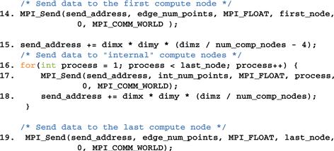
Figure 19.10 Data server process code (part 2).
Line 15 of Figure 19.10 advances the send_address pointer to the beginning of the data to be sent to process 1. From Figure 19.3, there are dimx∗dimy∗(dimz/num_comp_procs) elements in partition D1, which means D2 starts at a location that is dimx∗dimy∗(dimz/num_comp_procs) elements from the starting location of input. Recall that we also need to send the halo cells from D1 as well. Therefore, we adjust the starting address for the MPI_Send() back by four slices, which results in the expression for advancing the send_address pointer in line 15: dimx∗dimy∗(dimz/num_comp_procs-4).
Line 16 is a loop that sends out the MPI messages to process 1 through process np-3. In our small example for four compute processes, np is 5. The loop sends the MPI messages to processes 1, 2, and 3. These are internal processes that need to receive halo grid points for neighbors on both sides. Therefore, the second parameter of the MPI_Send() in line 17 uses int_num_nodes, that is, dimx∗dimy∗(dimz/num_comp_procs+8). The rest of the parameters are similar to that for the MPI_Send() in line 14 with the obvious exception that the destination process is specified by the loop variable process, which is incremented from 1 to np-3 (last_node is np-2).
Line 18 advances the send address for each internal process by the number of grid points in each partition: dimx∗dimy∗dimz/num_comp_nodes. Note that the starting locations of the halo grid points for internal processes are dimx∗dimy∗dimz/num_comp_procs points apart. Although we need to pull back the starting address by four slices to accommodate halo grid points, we do so for every internal process so the net distance between the starting locations remains as the number of grid points in each partition.
Line 19 sends the data to the process np-2, the last compute process that has only one neighbor to the left. Readers should be able to reason through all the parameter values used. Note that we are not quite done with the data server code. We will come back later for the final part of the data server that collects the output values from all compute processes.
We now turn our attention to the compute processes that receive the input from the data server process. In Figure 19.11, lines 1 and 2 establish the process ID for the process and the total number of processes for the application. Line 3 establishes that the data server is process np-1. Lines 4 and 5 calculate the number of grid points and the number of bytes that should be processed by each internal process. Lines 6 and 7 calculate the number of grid points and the number of bytes in each halo (four slices).
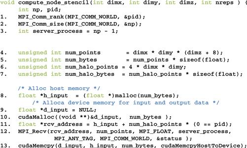
Figure 19.11 Compute process code (part 1).
Lines 8-10 allocate the host memory and device memory for the input data. Note that although the edge processes need less halo data, they still allocate the same amount of memory for simplicity; part of the allocated memory will not be used by the edge processes. Line 10 sets the starting address of the host memory for receiving the input data from the data server. For all compute processes except process 0, the starting receiving location is simply the starting location of the allocated memory for the input data. However, we adjust the receiving location by four slices. This is because for simplicity, we assume that the host memory for receiving the input data is arranged the same way for all compute processes: four slices of halo from the left neighbor followed by the partition, followed by four slices of halo from the right neighbor. However, we showed in line 4 of Figure 19.10 that the data server will not send any halo data from the left neighbor to process 0. That is, for process 0, the MPI message from the data server only contains the partition and the halo from the right neighbor. Therefore, line 10 adjusts the starting host memory location by four slices so that process 0 will correctly interpret the input data from the data server.
Line 12 receives the MPI message from the data server. Most of the parameters should be familiar. The last parameter reflects any error condition that occurred when the data is received. The second parameter specifies that all compute processes will receive the full amount of data from the data server. However, the data server will send less data to process 0 and process np-2. This is not reflected in the code because MPI_Recv() allows the second parameter to specify a larger number of data points than what is actually received, and will only place the actual number of bytes received from the sender into the receiving memory. In the case of process 0, the input data from the data server contains only the partition and the halo from the right neighbor. The received input will be placed by skipping the first four slices of the allocated memory, which should correspond to the halo for the (nonexistent) left neighbor. This effect is achieved with the term num_halo_points∗(pid==0) in line 11. In the case of process np-2, the input data contains the halo from the left neighbor and the partition. The received input will be placed from the beginning of the allocated memory, leaving the last four slices of the allocated memory unused.
Line 13 copies the received input data to the device memory. In the case of process 0, the left halo points are not valid. In the case of process np-2, the right halo points are not valid. However, for simplicity, all compute nodes send the full size to the device memory. The assumption is that the kernels will be launched in such a way that these invalid portions will be correctly ignored. After line 13, all the input data is in the device memory.
Figure 19.12 shows part 2 of the compute process code. Lines 14-16 allocate host memory and device memory for the output data. The output data buffer in the device memory will actually be used as a ping-pong buffer with the input data buffer. That is, they will switch roles in each iteration. We will return to this point later.
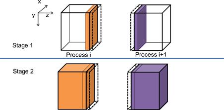
Figure 19.12 A two-stage strategy for overlapping computation with communication.
We are now ready to present the code that performs computation steps on the grid points.
19.5 Overlapping Computation and Communication
A simple way to perform the computation steps is for each compute process to perform a computation step on its entire partition, exchange halo data with the left and right neighbors, and repeat. While this is a very simple strategy, it is not very effective. The reason is that this strategy forces the system to be in one of the two modes. In the first mode, all compute processes are performing computation steps. During this time, the communication network is not used. In the second mode, all compute processes exchange halo data with their left and right neighbors. During this time, the computation hardware is not well utilized. Ideally, we would like to achieve better performance by utilizing both the communication network and computation hardware all the time. This can be achieved by dividing the computation tasks of each compute process into two stages, as illustrated in Figure 19.13.
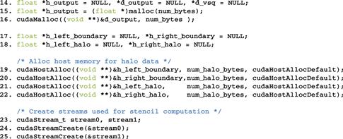
Figure 19.13 Compute process code (part 2).
During the first stage (stage 1), each compute process calculates its boundary slices that will be needed as halo cells by its neighbors in the next iteration. Let’s continue to assume that we use four slices of halo data. Figure 19.13 shows that the collection of four halo slices as a dashed transparent piece and the four boundary slices as a solid piece. Note that the solid piece of process i will be copied into the dashed piece of process i+1 and vice versa during the next communication. For process 0, the first phase calculates the right four slices of boundary data for four computation steps. For an internal node, it calculates the left four slices and the right four slices of its boundary data. For process n-2, it calculates the right four pieces of its boundary data. The rationale is that these boundary slices are needed by their neighbors for the next iteration. By calculating these boundary slices first, the data can be communicated to the neighbors while the compute processes calculate the rest of its grid points.
During the second stage (stage 2), each compute process performs two parallel activities. The first is to communicate its new boundary values to its neighbor processes. This is done by first copying the data from the device memory into the host memory, followed by sending MPI messages to the neighbors. As we will discuss later, we need to be careful that the data received from the neighbors is used in the next iteration, not the current iteration. The second activity is to calculate the rest of the data in the partition. If the communication activity takes a shorter amount of time than the calculation activity, we can hide the communication delay and fully utilize the computing hardware all the time. This is usually achieved by having enough slices in the internal part of each partition allow each compute process to perform computation steps in between communications.
To support the parallel activities in stage 2, we need to use two advanced features of the CUDA programming model: pinned memory allocation and streams. A pinned memory allocation requests that the memory allocated will not be paged out by the operating system. This is done with the cudaHostAlloc() API call. Lines 19-22 allocate memory buffers for the left and right boundary slices and the left and right halo slices. The left and right boundary slices need to be sent from the device memory to the left and right neighbor processes. The buffers are used as a host memory staging area for the device to copy data into, and then used as the source buffer for MPI_Send() to neighbor processes. The left and right halo slices need to be received from neighbor processes. The buffers are used as a host memory staging area for MPI_Recv() to use as a destination buffer and then copied to the device memory.
Note that the host memory allocation is done with the cudaHostAlloc() function rather than the standard malloc() function. The difference is that the cudaHostAlloc() function allocates a pinned memory buffer, sometimes also referred to as page-locked memory buffer. We need to present a little more background on the memory management in operating systems to fully understand the concept of pinned memory buffers.
In a modern computer system, the operating system manages a virtual memory space for applications. Each application has access to a large, consecutive address space. In reality, the system has a limited amount of physical memory that needs to be shared among all running applications. This sharing is performed by partitioning the virtual memory space into pages and mapping only the actively used pages into physical memory. When there is much demand for memory, the operating system needs to “page out” some of the pages from the physical memory to mass storage such as disks. Therefore, an application may have its data paged out any time during its execution.
The implementation of cudaMemcpy() uses a type of hardware called a direct memory access (DMA) device. When a cudaMemcpy() function is called to copy between the host and device memories, its implementation uses a DMA device to complete the task. On the host memory side, the DMA hardware operates on physical addresses. That is, the operating system needs to give a translated physical address to the DMA device. However, there is a chance that the data may be paged out before the DMA operation is complete. The physical memory locations for the data may be reassigned to another virtual memory data. In this case, the DMA operation can be potentially corrupted since its data can be overwritten by the paging activity.
A common solution to this corruption problem is for the CUDA runtime to perform the copy operation in two steps. For a host-to-device copy, the CUDA runtime first copies the source host memory data into a “pinned” memory buffer, which means the memory locations are marked so that the operating paging mechanism will not page out the data. It then uses the DMA device to copy the data from the pinned memory buffer to the device memory. For a device-to-host copy, the CUDA runtime first uses a DMA device to copy the data from the device memory into a pinned memory buffer. It then copies the data from the pinned memory to the destination host memory location. By using an extra pinned memory buffer, the DMA copy will be safe from any paging activities.
There are two problems with this approach. One is that the extra copy adds delay to the cudaMemcpy() operation. The second is that the extra complexity involved leads to a synchronous implementation of the cudaMemcpy() function. That is, the host program cannot continue to execute until the cudaMemcpy() function completes its operation and returns. This serializes all copy operations. To support fast copies with more parallelism, CUDA provides a cudaMemcpyAsync() function.
To use the cudaMemcpyAsync() function, the host memory buffer must be allocated as a pinned memory buffer. This is done in lines 19-22 for the host memory buffers of the left boundary, right boundary, left halo, and right halo slices. These buffers are allocated with a special cudaHostAlloc() function, which ensures that the allocated memory is pinned or page-locked from paging activities. Note that the cudaHostAlloc() function takes three parameters. The first two are the same as cudaMalloc(). The third specifies some options for more advanced usage. For most basic use cases, we can simply use the default value cudaHostAllocDefault.
The second advanced CUDA feature is streams, which supports the managed concurrent execution of CUDA API functions. A stream is an ordered sequence of operations. When a host code calls a cudaMemcpyAsync() function or launches a kernel, it can specify a stream as one of its parameters. All operations in the same stream will be done sequentially. Operations from two different streams can be executed in parallel.
Line 23 of Figure 19.13 declares two variables that are of CUDA built-in type cudaStream_t. Recall that the CUDA built-in types are declared in cuda.h. These variables are then used in calling the cudaStreamCreate() function. Each call to the cudaStreamCreate() creates a new stream and deposits a pointer to the stream into its parameter. After the calls in lines 24 and 25, the host code can use either stream0 or stream1 in subsequent cudaMemcpyAsync() calls and kernel launches.
Figure 19.14 shows part 3 of the compute process. Lines 27 and 28 calculate the process ID of the left and right neighbors of the compute process. The left_neighbor and right_neighbor variables will be used by compute processes as parameters when they send messages to and receive messages from their neighbors. For process 0, there is no left neighbor, so line 27 assigns an MPI constant MPI_PROC_NULL to left_neighbor to note this fact. For process np-2, there is no right neighbor, so line 28 assigns MPI_PROC_NULL to right_neighbor. For all the internal processes, line 27 assigns pid-1 to left_neighbor and pid+1 to right_neighbor.
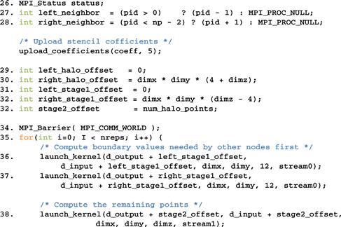
Figure 19.14 Compute process code (part 3).
Lines 31-33 set up several offsets that will be used to launch kernels and exchange data so that the computation and communication can be overlapped. These offsets define the regions of grid points that will need to be calculated at each stage of Figure 19.12. They are also visualized in Figure 19.15. Note that the total number of slices in each device memory is four slices of left halo points (dashed white), plus four slices of left boundary points, plus dimx∗dimy∗(dimz-8) internal points, plus four slices of boundary points, and four slices of right halo points (dashed white). Variable left_stage1_offset defines the starting point of the slices that are needed to calculate the left boundary slices. This includes 12 slices of data: 4 slices of left neighbor halo points, 4 slices of boundary points, and 4 slices of internal points. These slices are the leftmost in the partition so the offset value is set to 0 in line 31. Variable right_stage2_offset defines the starting point of the slices that are needed for calculating the right boundary slices. This also includes 12 slices: 4 slices of internal points, 4 slices of right boundary points, and 4 slices of right halo cells. The beginning point of these 12 slices can be derived by subtracting the total number of slices dimz+8 by 12. Therefore, the starting offset for these 12 slices is dimx∗dimy∗(dimz-4).
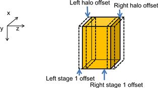
Figure 19.15 Device memory offsets used for data exchange with neighbor processes.
Line 35 is an MPI barrier synchronization, which is similar to the CUDA_syncthreads(). An MPI barrier forces all MPI processes specified by the parameter to wait for each other. None of the processes can continue their execution beyond this point until everyone has reached this point. The reason why we want a barrier synchronization here is to make sure that all compute nodes have received their input data and are ready to perform the computation steps. Since they will be exchanging data with each other, we would like to make them all start at about the same time. This way, we will not be in a situation where a few tardy processes delay all other processes during the data exchange. MPI_Barrier() is a collective communication function. We will discuss more details about collective communication API functions in the next section.
Line 35 starts a loop that performs the computation steps. For each iteration, each compute process will perform one cycle of the two-stage process in Figure 19.12.
Line 36 calls a function that will perform four computation steps to generate the four slices of the left boundary points in stage 1. We assume that there is a kernel that performs one computation step on a region of grip points. The launch_kernel() function takes several parameters. The first parameter is a pointer to the output data area for the kernel. The second parameter is a pointer to the input data area. In both cases, we add the left_stage1_offset to the input and output data in the device memory. The next three parameters specify the dimensions of the portion of the grid to be processed, which is 12 slices in this case. Note that we need to have four slices on each side. Line 37 does the same for the right boundary points in stage 1. Note that these kernels will be launched within stream0 and will be executed sequentially.
Line 38 launches a kernel to generate the dimx∗dimy∗(dimz-8) internal points in stage 2. Note that this also requires four slices of input boundary values on each side so the total number of input slices is dimx∗dimy∗dimz. The kernel is launched in stream1 and will be executed in parallel with those launched by lines 36 and 37.
Figure 19.16 shows part 4 of the compute process code. Line 39 copies the four slices of left boundary points to the host memory in preparation for data exchange with the left neighbor process. Line 40 copies the four slices of the right boundary points to the host memory in preparation for data exchange with the right neighbor process. Both are asynchronous copies in stream0 and will wait for the two kernels in stream0 to complete before they copy data. Line 40 is a synchronization that forces the process to wait for all operations in stream0 to complete before it can continue. This makes sure that the left and right boundary points are in the host memory before the process proceeds with data exchange.
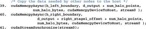
Figure 19.16 Compute process code (part 4).
During the data exchange phase, we will have all MPI processes send their boundary points to their left neighbors. That is, all processes will have their right neighbors sending data to them. It is, therefore, convenient to have an MPI function that sends data to a destination and receives data from a source. This reduces the number of MPI function calls. The MPI_Sendrecv() function in Figure 19.17 is such a function. It is essentially a combination of MPI_Send() and MPI_Recv(), so we will not further elaborate on the meaning of the parameters.
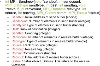
Figure 19.17 Syntax for the MPI_Sendrecv() function.
Figure 19.18 shows part 5 of the compute process code. Line 42 sends four slices of left boundary points to the left neighbor and receives four slices of right halo points from the right neighbors. Line 43 sends four slices of right boundary points to the right neighbor and receives four slices of left halo points from the left neighbor. In the case of process 0, its left_neighbor has been set to MPI_PROC_NULL in line 27, so the MPI runtime will not send out the message in line 42 or receive the message in line 43 for process 0. Likewise, the MPI runtime will not receive the message in line 42 or send out the message in line 43 for process np-2. Therefore, the conditional assignments in lines 27 and 28 eliminate the need for special if-the-else statements in lines 42 and 43.
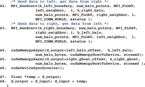
Figure 19.18 Compute process code (part 5).
After the MPI messages have been sent and received, lines 44 and 45 transfer the newly received halo points to the d_output buffer of the device memory. These copies are done in stream0 so they will execute in parallel with the kernel launched in line 38.
Line 46 is a synchronize operation for all device activities. This call forces the process to wait for all device activities, including kernels and data copies to complete. When the cudaDeviceSynchronize() function returns, all d_output data from the current computation step are in place: left halo data from the left neighbor process, boundary data from the kernel launched in line 36, internal data from the kernel launched in line 38, right boundary data from the kernel launched in line 37, and right halo data from the right neighbor.
Lines 47 and 48 swap the d_input and d_output pointers. This changes the output of the d_ouput data of the current computation step into the d_input data of the next computation step. The execution then proceeds to the next computation step by going to the next iteration of the loop of line 35. This will continue until all compute processes complete the number of computations specified by the parameter nreps.
Figure 19.19 shows part 6, the final part, of the compute process code. Line 46 is a barrier synchronization that forces all processes to wait for each other to finish their computation steps. Lines 50-52 swap d_output with d_input. This is because lines 47 and 48 swapped d_output with d_input in preparation for the next computation step. However, this is unnecessary for the last computation step. So, we use lines 50-52 to undo the swap. Line 53 copies the final output to the host memory. Line 54 sends the output to the data server. Line 55 waits for all processes to complete. Lines 56-59 free all the resources before returning to the main program.
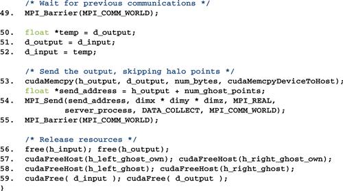
Figure 19.19 Compute process code (part 6).
Figure 19.20 shows part 3, the final part, of the data server process code, which continues from Figure 19.10. Line 20 waits for all compute nodes to complete their computation steps and send their outputs. This barrier corresponds to the barrier at line 55 of the compute process. Line 22 receives the output data from all the compute processes. Line 23 stores the output into an external storage. Lines 24 and 25 free resources before returning to the main program.
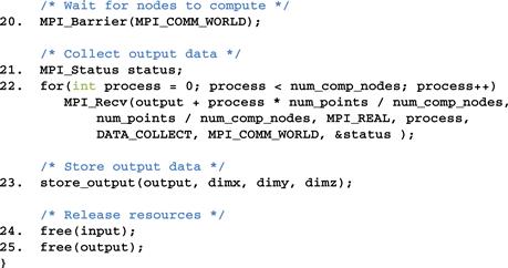
Figure 19.20 Data server process code (part 3).
19.6 MPI Collective Communication
The second type of MPI communication is collective communication, which involves a group of MPI processes. We have seen an example of the second type of MPI communication API: MPI_Barrier. The other commonly used group collective communication types are broadcast, reduction, gather, and scatter.
Barrier synchronization MPI_Barrier() is perhaps the most commonly used collective communication function. As we have seen in the stencil example, barriers are used to ensure that all MPI processes are ready before they begin to interact with each other. We will not elaborate on the other types of MPI collective communication functions but encourage readers to read up on the details of these functions. In general, collective communication functions are highly optimized by the MPI runtime developers and system vendors. Using them usually leads to better performance as well as readability and productivity.
19.7 Summary
We covered basic patterns of joint CUDA/MPI programming in this chapter. All processes in an MPI application run the same program. However, each process can follow different control flow and function call paths to specialize their roles, as is the case of the data server and the compute processes in our example in this chapter. We also presented a common pattern where compute processes exchange data. We presented the use of CUDA streams and asynchronous data transfers to enable the overlap of computation and communication. We would like to point out that while MPI is a very different programming system, all major MPI concepts that we covered in this chapter—SPMD, MPI ranks, and barriers—have counterparts in the CUDA programming model. This confirms our belief that by teaching parallel programming with one model well, our students can quickly pick up other programming models easily. We would like to encourage readers to build on the foundation from this chapter and study more advanced MPI features and other important patterns.
19.8 Exercises
19.1. For vector addition, if there are 100,000 elements in each vector and we are using three compute processes, how many elements are we sending to the last compute process?
19.2. If the MPI call MPI_Send(ptr_a, 1000, MPI_FLOAT, 2000, 4, MPI_COMM_WORLD) resulted in a data transfer of 40,000 bytes, what is the size of each data element being sent?
19.3. Which of the following statements is true?
a. MPI_Send() is blocking by default.
b. MPI_Recv() is blocking by default.
c. MPI messages must be at least 128 bytes.
d. MPI processes can access the same variable through shared memory.
19.4. Use the code base in Appendix A and examples in Chapters 3, 4, 5, and 6 to develop an OpenCL version of the matrix–matrix multiplication application.
Reference
1. Gropp W, Lusk E, Skjellum A. Using MPI: Portable Parallel Programming with the Message Passing Interface 2nd ed. Cambridge, MA: MIT Press, Scientific and Engineering Computation Series; 1999.