
In Chapter 5, “Naming and Addressing,” we looked at our understanding of naming and addressing. The main insights we took from that were Saltzer’s results and our insights about Saltzer as well as naming for applications and application protocols that followed from our understanding of the upper layers in Chapter 4, “Stalking the Upper-Layer Architecture.” In Chapter 6, “Divining Layers,” we realized that addresses were not quite what we thought they were: not just the names of protocol machines, but identifiers internal to a distributed IPC facility. In Chapter 7, “The Network IPC Model,” we assembled an architecture model based on what we had learned in the previous chapters, assembling the elements for a complete naming and addressing architecture. Then in Chapter 8, “Making Addresses Topological,” we considered what location dependent means in a network and showed how concepts of topology apply to addressing and, when used with a recursive architecture, can create a scalable and effective routing scheme.
Now we must consider a few other addressing-related topics: multihoming, multicast, and mobility. In the process, we will also consider so-called anycast addresses as the contrapositive of multicast. This will also provides the opportunity to apply this model to see what it predicts.
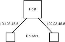
As related in the Preface and Chapter 5, the problem of multihoming raised its head very early in the history of networking and the ARPANET. As we saw by naming the point of attachment, the network could not tell that redundant connections went to the same place. To the network, two connections looked like two different hosts (see Figure 9-1). The host could make a choice of which interface to use when it opened a connection, thus providing some degree of load leveling. However, if one link to the router failed, so did all connections over it. Any traffic in transit to that host would be lost. This was a problem that the telephone system had not faced. The solution was clear: A logical address space was required over the physical address space.
For some reason, solving this problem never seemed a pressing matter to the Internet or its sponsors, which seems peculiar given that survivability was always given as a major rationale behind the design of the Net and seemingly what the DoD thought it was getting.[1] To recap our earlier brief discussion, many argued against implementing a solution if it imposed a cost on the entire network and because so few systems required multihoming that it was unfair to impose the cost on everyone. Of course, that small number of multihomed hosts were the ones that vast number of PCs needed to access! This lead to a deft piece of political engineering ensuring conditions in which no solution would be acceptable. As we have seen from Saltzer, there is no additional cost to supporting multihoming. Why wasn’t Saltzer’s paper applied? Who knows? It was certainly cited often enough. One gets the impression that there was more concern with protecting the status quo than making progress.
Others have argued that any multihoming would have to be with different providers on the assumption that one could not get multiple physical paths from the same provider. This, of course, is not true. Companies quite commonly buy redundant paths from the same provider. However, it is wise to physically check and recheck that the distinct paths being paid for actually are distinct, even if they are from different providers. The argument continues that it would be near impossible for the routing algorithms to recover and reroute a PDU destined for an interface on one provider’s network to another provider’s network. Although it is true that it is likely that either the hop count or the TCP retransmission timer would make delivery moot for PDUs nearing the failed interface, rerouting is not impossible. This argument assumes either that any interruption will be short-lived i.e., similar to the time to reroute or that the rather coarse-grained exchange[2] among providers that has existed in the past will continue to be the case. As local traffic increases,[3] so will the desire of providers to get traffic to other providers off their network at the earliest opportunity.
There was an opportunity during the IPng process to fix this problem. And frankly, many expected it to be fixed then. The developers of CLNP (ISO, 1993) and the OSI reference model had understood the necessity of naming the node rather than the interface. Because the problem had first surfaced in the ARPANET, it was always assumed it would be fixed in IP. So, it was quite surprising when in the IPng discussions it became apparent that so few IETF “experts” understood the fundamentals of network addressing that it would not be fixed. Naming the node was seen as something OSI did, so the Internet should not do it. And the opportunity was lost.
The multihoming problem has been ameliorated by the continuing progress of Moore’s law. Faster, cheaper processors and memory have kept the price of routers low enough that the increasing routing load was not painful. The argument was often made against developing a new solution, when the hardware was still quite capable of accommodating the problem. Of course, the problem with this argument is that the longer one waits to fix it, the more painful the day of reckoning. As computers tended more toward workstations and servers, the problem became less critical as the problem evolved from a host being multiply connected to a subnet being multiply connected. The existing methods were better at masking that problem. However, as we have seen, not having a solution for multihoming also applies to routers and increases the number of route calculations combinatorially. Later in this chapter, we will see how solving multihoming simplifies mobility, too.
As one would expect, the Internet has attempted to develop a number of workarounds (a politically correct word for kludge) for the lack of a multihoming solution. They run the gamut from being mostly spin to a genuine attempt to address the issue. All have their drawbacks. We consider a couple here before looking at how multihoming is supported by NIPCA. The least satisfying claim of multihoming support has been made by SCTP (RFC 3286, 2002; RFC 2960, 2000). The designers of SCTP use the well-known approach to solving the problem by simply changing the definition to something they can solve. It should be clear from the description of the earlier problem that there is nothing that a transport protocol can do about multihoming. The support SCTP provides is the ability to change the IP address (that is, the point of attachment [PoA]) without disrupting the transport connection. This is not possible in TCP because of the pseudo-header. TCP includes the source and destination IP addresses (as well as other fields from the IP header) in the TCP checksum.[4] Hence, should the IP address change, the checksum will fail, and the PDU will be discarded.
If the IP address named the node rather than the PoA, this would not be a problem. Changing the PoA would not affect the pseudo-header. The SCTP solution has no effect on responding to the failure of a PoA. If a PoA should fail, any traffic in transit will be discarded as undeliverable. The sending transport protocol machine would have to be cognizant of the routing change. In the current architectural approach, this would be difficult to do. Unfortunately, we must classify SCTP’s claims of supporting multihoming to be more in the nature of marketing than solving the problem.
The situation is quite different with Border Gateway Protocol (BGP) (RFC 1654, 1994; Perlman, 1992). BGP is an interdomain routing protocol. Because the multihoming problem is both an addressing issue and a routing problem, BGP at least stands a chance of being able to do something about it. For this discussion, I assume the reader has a basic knowledge of how interdomain routing works. To assume otherwise would require another chapter on that alone. Suffice it to say that BGP adopts a hierarchical approach to routing and groups collections of border routers into what are called autonomous systems (ASs). Routing information is exchanged about ASs. The solution to multihoming then is essentially to treat the AS as a node address. The host or site that wants to be multihomed acquires an AS number from its ISP and advertises routes to it via BGP. There are some drawbacks to this. The scope of BGP is the entire Internet. The intent of ASs was to serve as a means for aggregating routes among the thousands of ISPs that make up the public Internet. To also assign an AS to every host or site that wants to be multihomed significantly increases the routing burden on the entire Internet infrastructure. Consequently, some ISPs ignore the smaller ASs (that is, those that correspond to small sites or multihomed hosts), making it the same as if the AS were not multihomed. Clearly, although this approach solves the problem, it has scaling problems and is a band-aid to another problem. ASs are band-aids on top of the path-vector algorithm to allow it to scale to a large flat network like the current public Internet.[5] But the BGP solution does solve the problem by trying to emulate the right answer within the political constraints of current Internet.
Several other band-aids are used to provide solutions for multihoming. All are somewhere between these two. All increase the “parts-count” (that is, the complexity) to solve the problem or a part of it and complicate the solutions of other problems none of them scale, and none are really suitable for production networks, although they are used in them every day. Further, they only solve one particular part of the problem. They don’t make anything else easier. There is really no solution other than the one Saltzer proposed a quarter century ago.
Then in late 2006, a new crisis arose (Fuller, 2006; Huston, 2006). Router table size was on the rise again. The cause of the rise was laid at increased multihoming. Now that businesses rely heavily on the Internet, many more find it necessary to be multihomed. Based on estimates of the number of businesses large enough to potentially want multihoming, the conclusion was that we could not expect Moore’s law to solve the problem this time. This has led to much discussion and a spate of meetings to find another patch that will keep the problem at bay. The discussion has revolved around the so-called location/identifier split issue mentioned in Chapter 5. This only addresses part of the problem and does not solve it. As this book goes to press, a consensus has not been reached on the solution but probably will be by the time the book appears. Although for about ten days there was talk of solving the problem, but then more “pragmatic” heads prevailed. It appears that the consensus will be yet another band-aid. (Not to be cynical, but stopgap measures do sell more equipment than solving the problem.)
This is a problem that has been known for more than 35 years and ignored. It would have been much easier to fix 30 years ago or even 15 years ago. Not only fix but solve. What was it that Mrs. McCave said? Ensuring the stability of the global network infrastructure requires more vision and more proactive deployment than we are seeing. (It is curious that the major trade journals were silent on this topic for a year even though it was the hot topic at every IETF meeting that they covered.) This episode, along with a string of others, calls into question whether the IETF can be considered a responsible caretaker of the infrastructure that the world economy has come to rely on.
The model we have constructed here adopts Saltzer’s approach and generalizes it in the context of the recursive model. In keeping with our shift from a static architecture to a relative one, an (N)-address is a node address at the (N)-layer and a PoA address for the (N+1)-layer. In this architecture, the relation is relative (see Figure 9-2). Clearly, multihoming is supported as a consequence of the structure. If we had the right structure to begin with, we would probably never noticed there was a problem.[6] Routing is in terms of node addresses, with path selection (that is, the choice of the path to the next hop) done as a separate step.[7] Unlike the current Internet, NIPCA supports multihoming for both hosts and routers. This in itself significantly reduces the number of routes that must be calculated.[8] Furthermore, the recursive structure ensures that the mechanisms will scale.

The problems described earlier need not exist. The problem of coarse exchange between providers that we referred to earlier is driven primarily by “cost” (where cost is not just capital cost, but also the cost associated with meeting customer expectations of performance). As long as the amount of traffic for other providers is sufficiently low within an area that the cost of not exchanging within the area is cost-effective, providers won’t bother. If the amount of traffic increases, especially intraregion traffic for the other providers, the advantage of finer-grained exchange would gain advantage. Finer-grained exchanges might not be driven by the volume of traffic but by the need to ensure less jitter for voice and video traffic. Even so, a move to finer granularity of exchange is not helped by the fact that in general an inspection of the IP address will only indicate to a router what provider the address belongs to, not where it is. The application of topological addresses, as described at the end of Chapter 8, would further facilitate a move to finer granularity of exchange and would also facilitate rerouting to multihomed sites. Accommodating more fine-grained exchange in the address topology costs very little, and it doesn’t have to be used, but it does plan for the future in a manner unlike any from the past.
Multicast transmission has captured the imagination of networking researchers almost from the start of networking. Multicast is the ability to send a single PDU to a selected set of destinations, a generalization of broadcast (where broadcast is the ability for a sender to send a PDU that is received by all destinations on the network). Clearly, this derives from the wireless or multiaccess broadcast model. For the multiaccess media, the PDU generally has a special address value that indicates that the PDU is for all destinations. Because the media is multiaccess, all stations on the media see the broadcast or multicast address and determine whether to receive the PDU. This ancestry has led some researchers to assume multicast to be defined as purely one-to-many communication, and to coin the term multipeer to represent the more general many-to-many group communication one might require for various sorts of collaborative systems. We will use multicast for both unless there is a need to emphasize the difference.
Clearly, for inherently broadcast media, multicast is straightforward. But, multicast becomes a much more interesting problem in traditional wired network. Here it is generally implemented by computing a minimal spanning tree over the graph of the network generally rooted at the sender (see Figure 9-3). A PDU sent by the sender traverses the spanning tree being replicated only at the branching nodes of the tree. This saves considerable bandwidth. To send the same PDU to M destinations would normally require M PDUs to be sent. With multicast, M PDUs are delivered to M destinations, but the entire network does not have to carry the load of all M PDUs. Distributed spanning-tree algorithms were developed quite early. However, multipeer changes the problem: Rather than a different spanning tree rooted at each sender, one must find a single spanning tree that is optimal for the group of senders.
Although many proponents wax eloquent about multicast as a new and different distributed computing model, in the end it is ultimately a means for conserving bandwidth. Its primary importance is to the network provider in allowing it to carry more traffic using fewer resources and manage it better. The advantage to the user is minimal.
This is where the simplicity of the problem ends. There are a myriad of complications, whose intellectual challenge has generated extensive literature on the subject. However, multicast has not found much adoption outside the research community. The complexity and overhead of setting up multicast groups combined with the precipitous drop in bandwidth costs have continued to make the brute-force approach of sending M copies over M connections acceptable. As applications that could use multicast continue to grow, however, especially in the area of multimedia, we can expect that even with the advances in fiber, the need to make more effective use of bandwidth will reassert itself, and the complexity and cost of managing M pairwise connections will exceed the cost of managing multicast groups; so, multicast may find greater use. Of course, anything that can be done to simplify multicast deployment can only help.
Most of the research has concentrated on particular applications and provided solutions for each particular problem, with little or no consideration of how that solution would work along with other multicast applications with different requirements. However, because multicast is primarily a benefit to the provider rather than the user, a provider is going to want a solution that covers many multicast applications. If every class of application that could use multicast requires a different solution, this would be a nonstarter. We will not even try to survey the literature[9] but will refer to key developments as we proceed. We want to use this experience in traditional networks as data and hold it up to the structures we have developed here to see how it either improves or simplifies or complicates the problem.
The first problem with multicast (one ignored by most researchers) is that there are so many forms of it. It is fairly easy to construct a list of characteristics, such as the following:
Centralized versus decentralized (Multicast or multipeer?)
Static versus dynamic population (Can the membership change with time?)
Known versus unknown population (Members may be unknown with wireless?)
Isotropic versus anisotropic (Do all members behave the same?)
Quorum (Is a minimum membership required?)
Reliable versus unreliable
Simplex versus duplex
And so on
Within these characteristics are multiple policies that might be used, making the range of potential protocols quite large. One would not expect a single solution to effectively accommodate the entire range. But to create specific solutions for specific applications would lead to proliferation and complexity within the network. Providers are not enthusiastic about introducing another parallel routing system, let alone many. But perhaps not all combinations would find applications. Perhaps a small number would cover the major applications.
The latter assumption turns out to be wrong. One of the myriad standards organizations to look at multicast actually took the time to explore the matrix of multicast characteristics. It expected to find clusters of applications for some parameters and others that clearly would not occur. It fully expected to find that a small set of characteristics covered the great majority of cases (a common result in engineering, allowing the designer to concentrate on the important combinations rather than a fully general solution). Although there were a very few combinations for which it was unlikely to find an application, quite likely scenarios could be found for the vast majority of combinations. Not a welcome result.
Just with the connection/connectionless problem, we need to consider the service of of multicast and the function of multicast separately. Multicast is viewed as communication with a group (a set of users). Some models assume that all participants are members of the group (that is, multipeer). Others assume that the group is an entity that others outside the group communicate with (that is, multicast)—in a sense, unicast[10] communication with a group. This difference will be most pronounced in the consideration of multicast naming (see the following section). In the literature on multicast, one will generally find a service model that differs from the model for unicast communication. The sequence of API calls required is different. The application must be aware of whether it is doing multicast.
In the traditional unicast model, communication is provided by primitives to connect, send, receive, and disconnect, executed in that order. (Here we have replaced connect with allocate to include initiation of connectionless communication.) In multicast, the service primitives are generally connect, join, leave, send, receive, and disconnect.
The connect primitive creates the group and makes the initiator a member. Join and leave are used by members of the group to dynamically join and leave the group. Disconnect is used to terminate participation in the group. There is some variation in how the initiator may leave the group without terminating it. This, of course, creates a different sequence of interactions than unicast. The application must be cognizant of whether the communication is unicast or multicast, just as we saw earlier that the user had to be cognizant of whether the communication was connection or connectionless. In this model, a multicast group of two members is different from a unicast communication. We would clearly prefer a model in which one collapses cleanly into the other. Or more strongly, why should the application have to be aware of multicast at all?
But notice that the primary purpose of the “connect” primitive is creating the group, essentially creating sufficient shared state within the network to allow an instance of communication to be created. This is what we have called the enrollment phase. In fact, if the service model is recast so that creating the group is an enrollment function, join and leave become synonymous with connect and disconnect. The initiator would issue a primitive (enroll) to create the multicast group and in a separate operation initiate communication with the group with a join/connect/allocate/attach. Hence, the interaction sequence (that is, the partial state machine associated with the service interaction) is the same for multicast as for the unicast and connectionless cases. In fact, the only difference would be that the destination naming parameter would name a set of names rather than a single name (or is that a set of one element?). Furthermore, it is consistent with our model and eliminates another special case. We have found an effective single model for all three “modes” of communication: connectionless, connection, multicast.
As always, the problems surrounding naming and addressing are subtle and often less than obvious. There have been two models for multicast addressing. What has become the generally accepted definition is that a multicast “address” is the name of a set of addresses, such that referencing the set is equivalent to referencing all members of the set.
Initially, the Internet adopted a different definition. The early Internet multicast protocols viewed a multicast address as essentially an ambiguous or nonunique address. Simply viewed, several entities in the network had the same address so that a PDU with a multicast address was delivered to all interfaces with that address. This is an attempt to mimic the semantics of broadcast or multicast addresses on a LAN: Multiple interfaces on a LAN have the same (multicast) address assigned to them. As a PDU propagates on the LAN with an address (of whatever kind), the interfaces detect the PDU and read its address. If the address belongs to this interface, the PDU is read. In effect, if more than one station on the Ethernet has the same address, it is multicast.
This is straightforward with LANs, but for other technologies it means we have to ensure that every node sees every PDU. This means that flooding is about the only strategy that can be used. Flooding is generally considered pathological behavior. Instead of reducing the load on the network, it increases it. This is not good. Essentially, multicast in this model is broadcast, which is then pruned. This defeats the advantage of multicast of saving bandwidth in the network. It does retain the advantage that the sender only sends the PDU once rather than M times. Not much of a savings. Why can’t we use a spanning tree as with other schemes? A spanning tree would require a correspondence between a normal address and the multicast group name. For all intents and purposes, this would bring us back to the set model of the address stated earlier. Flooding as a distribution mechanism does not scale and is not greeted by providers with enthusiasm.
The other peculiarity of this early Internet model was that it was built around what we referred to earlier as “unicast communication to a group.” The sender is generally not part of the group but is sending PDUs to a group. This would seem to presume a simplex communication model—best suited for a “limited broadcast” model rather than the kind of more general distributed computing models required by multipeer applications. Also, the inability to resolve the multicast address to a unicast address has negative security implications. Given its problems, it is odd that this definition ever arose considering the earliest work (Dalal, 1977) on multicast used the set definition of a multicast address.
We must consider one other somewhat pedantic issue related to multicast addresses: They aren’t addresses. As we have defined them, addresses are location dependent. Multicast “addresses” are names of a set. The elements of the set are addresses, but the name of the set cannot be.
The concept of location dependent that we wanted was to know whether two addresses were “near” each other—so that we knew which direction to send them and whether we could aggregate routes. Although one could attribute the smallest scope of the elements of the set with the concept of a “location,” this seems to be not only stretching the spirit of the concept, but also not really helpful either. At first blush, one thinks of nicely behaved sets and how the concept of location would apply to them. But it doesn’t take long to come up with quite reasonable “monsters” for which it is much less clear how the concept would apply. It is far from clear what utility this would have. The most location dependence a multicast address could have would have to be common to the entire set. But this property will arise naturally from the analysis of the members of the set and in the computation of the spanning tree. It might be of some utility to nonmembers attempting to communicate with the group, but here again this would have only limited utility to route PDUs to some idea of the general area of the group (if there is one). Multicast distribution relies on one of two techniques, either some form of spanning tree or the underlying physical layer is inherently multiaccess, a degenerate spanning tree. In either case, what a sender external to the group needs to know is where the root of the tree is, or where it can gain access to the group (not some vague idea of the area the group is spread over). There is not much point in having a multicast address (that is, location dependent). They are simply names of sets of addresses.
The conclusion we are drawn to is that multicast addresses, although they may be represented by elements from an address space, are semantically names. We will use the term multicast name throughout to remind ourselves that these are not location-dependent names (that is, not addresses). To be very precise and in keeping with the model we have developed here, the application would have a multicast application name defined as a set of application names. We have already defined this: a distributed-application-name. Interesting, isn’t it? This would be passed in an open request to the DIF, which would allocate a multicast name from the DIFs address space. This multicast name would name the set of addresses to which the applications were bound. (Rules for adding or deleting addresses from the set would be associated with the set.)
The primary focus of multicast research has been on solving the multicast distribution problem at the network layer for networks without multiaccess physical media. Many approaches have been tried, including brute-force flooding. But most of the emphasis has been on distributed algorithms for generating spanning trees. Not only is this much more efficient, it is also an intellectually challenging problem. The first attempt to solve this was Yogen Dalal’s Ph.D. thesis (1977). Since then there are have been many theses and papers. Although there has been some emphasis on pure multicast (that is, a single sender to a group), much of the interest has been on “multipeer,” where each member of the group would be communicating with the group. This has led to several problems:
Scaling the techniques to support large groups
Maintaining an optimal or near-optimal spanning tree when the members of the group change
Reducing the complexity of multipeer by not requiring the computation of a separate spanning tree for every member of the group
This has led to a number of standard multicast protocols being proposed: DVMRP (RFC 1075, 1988), PIM (RFC 2362, 1998; Estrin et al., 1996) and CBT (RFC 2189, 1998). The focus of these algorithms is to find optimal spanning trees given multiple senders in the group. Hence, the root of the spanning tree is not at one of the senders, but at some “center of gravity” for the group. The problem then becomes finding that center of gravity. We will not review these techniques here. They are more than adequately covered in numerous textbooks. The major problem confronted by most of these is the complexity of the computation in current networks with large groups.
This would be a good place to consider how these names work. The heading of this section uses the term Sentential because we will be concerned with the two forms of sentential naming that we find: universal and existential.[11] We have just covered the “universal” naming operator (that is, multicast). We will also consider the “existential” naming operator, known colloquially in the field as an “anycast” name.[12] We can define an anycast name as the name of a set such that when the name is referenced one element of the set is returned according to some rule associated with the set.
In both cases, the use of the sentential name resolves sooner or later to an address. This then raises the question of when does this name resolution take place. With the anycast name, it may be immediate or at various points along the path, whereas with a multicast name it will be done at several points along the way. We would like an answer that minimizes special cases. This leads to the following:
The rule associated with the set is applied when the forwarding table is created to yield a list of addresses that satisfy the rule. When a PDU with a sentential destination address is evaluated at each relay, it is then sent to the elements of the list. (Of course, a list can have one element.)
The sentential names are placeholders for the set and its associated rule. At each relay (hop), the set is evaluated according to the rule. For anycast, this means selecting an address from the set and forwarding toward that address. For multicast, it means selecting the addresses downstream on this spanning tree and forwarding a copy of the PDU toward all of them. Given topological addresses, the addresses in the multicast set can be ordered into a virtual spanning tree based on the topology of the address space. (The structure of the addresses would imply a spanning tree or, more precisely, which addresses were near or beyond others.) This then simplifies the task of each node, which given its own address knows where it fits in the spanning tree of that multicast set and which branches it must forward copies of the PDU on. In fact, with a reasonable topological address space, the addresses of the nodes of the spanning tree can be approximated. This implies that specialized multicast protocols are unnecessary. We still need the distributed spanning-tree algorithms. The definition of the sets will have to be distributed to each member of the DIF along with the policies associated with it and the spanning-tree algorithm applied. This information is then used to generate entries in the forwarding table. The only difference being that a forwarding table’s lookup results comprise a list, admittedly a list with one element most of the time, but a list just the same.
Sentential addresses are used in building the forwarding table. The rule is only evaluated when the forwarding table is generated. Any changes in network conditions that would change the outcome of the rule are equivalent to the same conditions that would cause a recalculation of the forwarding table. In the multicast case, this means determining to which branches of the spanning tree the PDU is to be forwarded. For an anycast address, this means the PDU is forwarded toward the address returned by the rule associated with the set. (This of course implies that the rule could yield different results at different nodes along the route. This envisions a concept of anycast that is both simpler and more powerful than allowed by IPv6.)
Unicast is a subset of multicast, but multicast devolves to unicast.
A multicast group at layer N, (N)-G, is defined as a set of addresses, {(N)-Ai}, such that a reference to (N)-G by a member of the group yields all elements of {(N)-Ai}. It is sometimes useful to consider traditional “unicast” data transfer as a multicast group of two. (N)-G is identified by an (N)-group-address, (N)-GA.
(N)-group-name ∀ (N)-Ai ∋ (N)-Ai ∈ G = {(N)-Ai} |
The order of an (N)-G (that is, the number of elements in the set) is |{(N)-Ai}| or |(N)-G|.
Although there is no logical reason that the set cannot contain a group name, there are practical reasons to be cautious about doing so (for example, duplicates).
The primary purpose of multicast is to reduce load on the network for those applications that require the same data be delivered to a number of addresses. Several mechanisms are used to accomplish this ranging from brute-force flooding to the more subtle forms of spanning trees. These spanning trees may be rooted at the sender(s) or at some intermediate point, sometimes referred to as the “center of gravity” or “core” of the group.
A minimal spanning tree is an acyclic graph T(n,a) consisting of n nodes and a arcs imposed on a more general graph of the network. This tree represents the minimal number of arcs required to connect (or span) all members of (N)-G. The leaf or terminal nodes of the tree are the elements of the set {(N)-Ai}. The nonterminal nodes are intermediate relays in the (N)-layer. Let’s designate such a spanning tree for the group, G as TG(n,a). Then the bounds on the number of nodes in the spanning tree are given by the following:
min |TG(n,a)| = |{(N)-Ai}| |
max |TG(n,a)| = |{(N)-Ai}| + (d-1) |{(N)-Ai}| |
where d = diameter of the network |
Let (N)-B be a group name and (N)-Ai be the addresses in the group, then
∃ a spanning tree, (N)-TB(Ai, ci) which covers (N)-B. |
∀ (N)-Ai ∈ (N)-B, ∃ (N – 1)-Ai ∋ F:(N)-Ai ⇒ (N – 1) Ai and (N – 1)-Ai ∈ |
(N – 1)-Gi |
Or some elements of (N)-B such that (N)-Ai is bound to (N – 1)-Ai. This binding creates a group at layer (N – 1) in each of these subnets. In current networks, F is 1:1, ∀ Ai. This may or may not be the case in general.
∀ (N – 1)-Ai ∃ m subnets, Si ∋ (N – 1)-Ai ⊇ Si |
If | (N – 1)-G | = k, then ∃ m Si ∋ ∀(N – 1)-Ai ∈ (N – 1)-G, m ≤ k |
As we saw previously, to the user of layer N there is one “subnet,” a user of layer (N), that appears directly connected to all other users of that layer. From within the (N)-layer, there are m subnets connected by the (N)-relays. A subset of these (N)-relays form the nonterminal nodes of the spanning tree, (N)-T(Ai,ci). Thus, there are k addresses that belong to m subnets with m ≤ k. This decomposes the (N)-TB(Ai,ci) into m(N−1)-TB(Ai,ci).
Let {(N−1)-Ai}j be the (N−1)-Gj of addresses in subnet Sj |
At the m(N−1)-layers, ∃(N−1)-Gj ∋ {(N - 1)-Ai}j |
(N)-GA is supported by the services of the (N−1)-layers (subnets) that form a covering of the (N)-layer. A subset of this covering provides services in two distinct ways (see Figure 9-4):
The p end subnets,
 , {(N−1)-Ai}j
The m – p transit subnets,
 , that connect the p end subnets
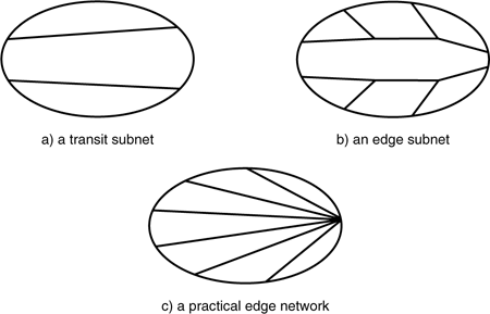
Figure 9-4. In a recursive architecture, multicast groups decompose into two cases: a) transit subnets that are unicast, and b) edge subnets, which use spanning trees. Practically, however, the latter case is simpler if c) unicast flows from the border router are used with no internal branching (making multicast distribution a subset of unicast routing.)
The spanning tree of the end subnets would be rooted at a border relay at which it enters the subnet. The (N)-GA is supported by p (N−1)-Ge and (m–p)G.
Note there may be more than one such entry point and thus more than one independent spanning tree for the same group in the same subnet.
As one moves down through the layers, the number of end subnets decreases, the degree of branching decreases, and the number of transit subnets increases.
Multicast has always been considered such a hard problem that multiplexing multicast groups for greater efficiency was just too much to consider. But given an approach that allows us to decompose the problem, multiplexing becomes fairly straightforward. There are two cases that must be considered: transit groups and end groups.
Assume layer N has m subnets. Any group from layer (N+1) will be decomposed into n segments n ≤ m consisting of p end groups and q transit groups, n = p + q. Suppose there are k such groups at the (N+1)-layer, each with its own value of n, p, and q.
The number of subnets is much smaller than the number of hosts participating in the group, as is the number of (N)-relays. Therefore, it is likely that there will be a number of transit groups that have flows between the same (N)-relays. These are candidates for multiplexing.
A transit group is distinguished by connecting only (N)-relays. A transit subnet group consists of q pairwise connections, where 1 ≤ q ≤ m. The decision to multiplex them will be no different than for any other unicast flow.
An end group is rooted at (N)-relay, and leaf nodes are either end systems or other (N)-relays. Multiplexing the spanning trees of the end groups is more difficult. One could require that the trees be the same, but this would not lead to many opportunities to multiplex. It would be better to allow similar trees to be multiplexed, the only question is what does “similar” mean.
Here we have a number of spanning trees rooted at the same (N)-relay. To multiplex; we will want (N)-Ge with similar if not the same tree. Let’s define λ-similarity, as λ is the number of leaf nodes of the G1 ... Gk have in common. Suppose G1 ... Gk are the end groups of an (N)-subnet of distinct (N+1)-groups, then
∀ Gi ∈ G1 ... Gk < λ then Gi may be multiplexed. |
Then construct a spanning tree for >> G1 ... Gk. This will cause some PDUs to be delivered to addresses that are not members of the group and so be discarded. (Other QoS parameters may cause Gi to be multiplexed with a different (N)-Gi.)
One of the first problems researchers took up along with multicast distribution was multicast transport. If the multicast distribution algorithms were the network layer, then what did the mechanisms look like for a multicast transport protocol to provide end-to-end reliability? It was a natural topic to pursue. Can we adapt protocols like TCP to provide reliable multipeer? This has been a favorite topic with tens of proposals, a great thesis generator. However, this proves to be a less-than-straightforward problem.
Just defining what service multicast transport provides is problematic before one even gets to considering the mechanisms for providing it. Consider the following issues:
What is done if one member falls behind and can’t accept data fast enough? Is everyone slowed down to the same rate? Is data to the slow ones dropped? Is the slow member dropped? Is data for the slow one buffered? For how long?
Is retransmission to all members of the group or just the ones that either nack’ed or timed out? If the latter, doesn’t this defeat the advantage of multicast? By making it into (m-1) unicast connections?
What happens if one member doesn’t receive something after several retries? Drop the member? Terminate the whole group?
Can multiple senders send at the same time? If so, what order is maintained if there are multiple senders in the group? Relative? Partial ordering? Total ordering? No order?
If the group has dynamic membership and a new member joins, at what point does it start receiving data? If it leaves and rejoins, is the answer different?
The list can go on and on. It doesn’t take long to realize that most, if not all, of these may be desirable by some application. The design of a single protocol or even a small number of related protocols satisfying the range indicated by these questions is a daunting problem. Of course, the strategy of separating mechanism and policy developed here can be used to address this at least partially.
The problems don’t stop there. A prime characteristic of error- and flow-control protocols is that they have feedback mechanisms. Feedback is inherently pairwise. This brings us to the other problem with multicast transport: ack implosion. What is the point of multipeer distribution if the error- and flow-control protocol is going to impose a service of (m–1) pairwise connections? The senders must keep separate state information for each receiver in the group so that it knows who has received what and how fast it can send. But weren’t we trying to avoid the burden of keeping track of each member of the group? If each sender must maintain state for each receiver, multicast will reduce load on the network but not for the sending systems.
Acknowledgment and flow control are feedback mechanisms and thus return information to the sender. For a multicast group, this means that for a group of m members (m – 1) acks or credits will need to be sent back for the sending protocol machine to process. Do these pairwise acks destroy the group nature of the communication? One can easily imagine that for large values of m the sender could become overwhelmed by feedback PDUs. (Ack implosion has become the shorthand term for this problem, even though it involves both ack and flow-control information.) Does this mean there needs to be flow control on the flow-control PDUs? Many proposals have considered techniques that aggregate the control messages as they return up the spanning tree (thus reducing the number of control PDUs the sender must see). In traditional architectures, this was problematic. The aggregation function of the transport protocol required knowledge of the spanning tree in the layer below. Furthermore, the transport protocol is relaying and processing PDUs at intermediate points. Doesn’t aggregating break the “end-to-end”-ness of the transport protocol? What happens if an aggregating mode fails? Also, does the process of aggregating impose a policy with respect to systems that fall behind, and so on? It also raises the question of whether it really saves anything. Is this a step back to X.25-like hop-by-hop error and flow control? It reduces the number of PDUs received, but the amount of information must be close to the same. Consider the following:
What the sender needs to know is what sequence number is being ack’ed and by whom. The aggregated ack might contain the sequence number and the list of addresses and port-ids corresponding to all of the receivers who have ack’ed this. The list can’t be assured to be a contiguous range, so the aggregated Ack PDU must be able to carry the list of port-ids, perhaps representing ranges as well as individual ports. This reduces the number of control messages being delivered (probably fixed format), but it is doubtful it reduces the processing burden or reduces the memory requirements. Nor have we considered the delay and processing overhead incurred by aggregating. Are acks held at interim spanning tree nodes to await PDUs that it can be aggregated with? Does this mean that these nodes must keep track of which acks have been forwarded? Or one could assume that each node collects all downstream acks, and so only a single ack for all the members is finally delivered to the sender. Now we are up against the slow responder. This implies a fixed timeout interval for all members so that any member that didn’t respond within the time interval was assumed to have not gotten the PDU and is a candidate for retransmission or being dropped from the group. As one moved in the reverse direction up the spanning tree, the timeout for each node would have to be progressively longer to allow for the delay by nodes lower in the tree. This could lead to much longer retransmission timeouts than seen for pairwise connections, but that might be acceptable. Do retransmissions go to everyone or just the ones that didn’t report? This strategy is possible for acknowledgment, but flow control is a bit different. What does one do about members who are slow? A member may be delayed a considerable amount of time. Is traffic stopped by one member of the group? Etc. etc.
As you can see, the questions surrounding a reliable multicast protocol are legion. Those proposed in the literature have generally been designed for a specific environment where specific choices can be made. Separating mechanism and policy can cover some of this variability. It remains to be seen whether it can or should cover it all. In the structure developed here, the error- and flow-control protocol and the relaying and multiplexing process are in the same DIF and can share information. Because the EFCP is structurally two protocols, the Control PDUs could be routed separately from the Transfer PDUs. One spanning tree could be used to support data transfer, while a separate parallel spanning tree supports the control flow with protocol machines at each node aggregating them as they percolate back up the tree.
In the NIPCA structure, this is not a layer violation because the EFCP and relaying process are in the same DIF/layer. In fact, it actually fits rather nicely. However, a major design consideration of EFCPs to ensure end-to-end integrity is that its PDUs are interpreted only at the “ends,” not by intermediate points. Aggregating acks (and credits) is not a “layer violation,” but simply combining PDUs, a well-accepted mechanism of the relaying and multiplexing function of a layer. However, to do more (that is, combining the semantics of the acks and credits to reduce the number of actual PDUs) does raise questions about the end-to-end integrity of the protocol. Most multicast applications can tolerate some loss (that is, streaming video or voice). One might consider a stock ticker, but given the timeliness of the data it could not tolerate the retransmission delays either. Assuming that there are applications that will arise for reliable, it seems that we need to review and possibly refine the theory of EFCPs with respect to the degrees of integrity and the role of intermediate processing.
Interpreting multicast and anycast in terms of a distributed IPC architecture makes many things more clear. We have been able to integrate multicast into the operation of the layer such that the application sees the same interface at the layer boundary. The only difference is that when the application requests communication, it passes the name of a set rather than the name of an application. Of course, we could interpret it as always being a set—just that often the set has one element. We have also found that it is fairly easy to architecturally integrate multicast and anycast operation into routing. Given that the set of potential routes from any given router is a spanning tree, future research will undoubtedly increase the degree of integration. We also found that in a recursive architecture, multicast can be limited to border routers and hosts, further simplifying the problem and opening the door to multiplexing multicast trees, which not only allows greater transmission efficiency but also reduces the complexity of its support.
NIPCA also sheds light on the nature of reliable multicast. We won’t be so bold as to say that NIPCA solves all the problems. It is fairly clear that as long as tightly coupled feedback mechanisms are used to create reliable protocols, the problems of reliable multicast are inherent. The separation of mechanism and policy does make it possible to accommodate much if not all of the range of reliable multicast. The structure of the DIF (three loci of processing with different duty cycles) would appear to neatly accommodate ack aggregation at the border routers. (Similarly, I will use ack aggregation as a shorthand for aggregating ack or flow-control feedback information being returned to the sender.) As we saw, we could map multicast data transfer and multicast “control” to separate spanning trees. In this case, normal operation would allow for aggregating acks and credits at they flow back up the tree to the sender.
What is questionable is doing any more “compaction” (that is, having a single ack reflect the ack of several ends). This would seem to drag the model to a hop-by-hop paradigm, rather than our preferred end-to-end paradigm for error control. Why is this bad? Partly because this is error control in adjacent layers with nominally the same scope. Why do the same thing twice? What did the layer below miss what the layer above is detecting? This is imposing a policy about the nature of ack and credit across multiple endpoints. This may be the desired policy. And we can create a very reasonable rationale, such as “any policy that can be performed by the source that can be distributed transparently among the IPC processes in the DIF.” In other words, any operation can be performed on EFCP Control PDUs that does not modify the state vector. Unicast is then a degenerate case where the function is null.
This would seem to avoid the concerns that ack aggregation impairs the “end-to-end” nature of an EFCP. Any “impairment” of end-to-end-ness (determining what to do with delayed acks, and so on) is a matter of policy, and policy is a parameter selected based on what the application has requested, and any action that changes the state vector is only being done at the “ends.” In terms of assembling a theory, we would like a better rationale. Was our traditional view of the end-to-end-ness of an EFCP—that acks are simply relayed to the source and not interpreted along the way—focused on a special case? Is multicast the general case that we must consider. Being able to relate such rationale to a consequence of the fundamental structure would be more assuring that there was truly some basis for such rationale and it wasn’t just an expedient. Is this it?
But at the same time, the wide range of special cases generated by reliable multicast seems to indicate that they are all kludges and multicast is purely a routing and distribution phenomena. Recognizing that this is computer science, so that most anything can be made to work, one still is unsure whether feedback mechanisms should not be part of multicast.
Mobility has become a hot topic in networking. Although mobility does present some new issues, they turn out to be either more of the same or requirements to be more explicit and formal about things we were already doing or should have been. There are basically three common forms of mobility:
Mobile network systems appear more difficult than they are because we didn’t finish building the basic architecture before moving on to consider mobility. Mobile applications by their nature are confined to the periphery of a network or to relatively small standalone networks or subnets. But as always, many view mobility as an opportunity for new special cases, rather than as an application of a general model. This is not helped by the way that mobility must be supported in the Internet owing to its incomplete addressing architecture.
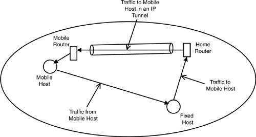
To support mobility in IP (see Figure 9-5; Perkins, 1998), a router in the “home subnet” of a mobile host is assigned the role of a “home router.” The mobile host’s IP address, S, in that subnet continues to identify the mobile host; but when it moves into the new subnet, it is assigned a local IP address, M, in that subnet. An IP tunnel is created between the home router and a router in the new subnet with a direct connection to the mobile host. When PDUs are sent to the mobile host with the IP address S, they are routed to the “home router”; the home router knows the mobile host is not where it is supposed to be; so the PDU is encapsulated and sent down the IP tunnel to the foreign subnet. There the PDUs are forwarded on the interface that connects the mobile host to the foreign router. The foreign router knows that traffic from the tunnel is to be forwarded to the IP address of the mobile host that is on a known local interface of the foreign router. Traffic from the mobile host to the sender can take a more direct route or can be funneled back through the tunnel. The mobile host’s IP address is only used by the home router and by the mobile router. These two know the mobile host was or is directly connected to them. They must know that this address requires special handling.
Mobile routers and home routers are special cases and would have to be identified in advance. Furthermore, there are two single points of failure: the home router and the foreign router. If either fails, communication is lost. This approach is more suitable for “static” mobility, where a mobile host is removed from the network at one point and reattached at another temporarily. It is less suitable for roaming, where the mobile host is moving and the IP tunnel from the home router has to follow it. (It is done, but relies on the fact that MAC addresses have greater scope than IP addresses and don’t change.)
Why is IP mobility so complicated? As we have seen, in the Internet architecture the IP address is the only means for identifying anything. Well-known sockets are extensions of IP addresses and not independent of them (although there is a global location-independent host name that is mapped to the IP address by DNS). For purposes of mobility, domain names are synonyms for the IP address; they do not name a distinct object. The update time for DNS, averaging 8 to 12 hours globally, is far too long for updating IP as a point-of-attachment address.
The telephone system initially had a similar problem when they began to consider mobile phone service. As noted earlier, in the telephone system the phone number was the name of the wire coming from the central office to the phone. This would clearly not work for a mobile system. The handset would need to establish communication with a cell tower. As the handset moved, the cellular system would have to follow the handset and hand it off from tower to tower. The phone number would have to name the handset because that was what one would call. (Already we are in better shape.) The cell phone system would need a distinct address space for the cell tower antennas. The telephone number identified the handset (a node address) that was communicating at a lower layer with a cell tower (PoA). As the cell phone moved around its area, it communicates with one cell tower after another, often to more than one at a time (multihoming). It is doubtful the cell phone developers realized that in networking terms they were being forced to make a distinction between node address and PoA address, but they were.[13]
Cell phone use was initially restricted to a local area, just as the phone system was in its early days. If a cell phone user left his “home” area, special arrangements had to be made for “roaming” (for an additional charge). Entries were made in a special roaming database called the Visitor Locator Register (VLR). As cell phone use increased, so did the number of people needing to roam. Travelers making special arrangements every time they were about to jump on a plane quickly became unworkable. Cellular systems needed to allow any phone to roam outside its home area without human intervention.
Clearly people’s phone numbers couldn’t change, but cell phone providers needed a more effective way of finding the handset when it wasn’t where it was suppose to be. This meant that the phone number in the handset would not indicate where the phone was. The phone numbers would become location independent. (We have seen this before.) Without disrupting their customers, the cell phone operators jacked up their architecture (again), making node addresses of phone numbers, application names, and other newly assigned numbers. Contrary to how this might have looked at the time, this wasn’t that big of a change. The phone system had already been purposely confusing phone numbers as both node addresses and location-independent names (that is, application names) with 800 numbers and 411 and 911 numbers. In one’s home area, it was likely that one’s application name and node address were the same string of bits; as the phone moved beyond its home area, however, the node address was changed to one local to the new area, but the phone number seen by the user (and those calling her) remained the same. The cell phone system merely changed the mapping in its directory databases so that connect requests to the application name are routed to the subnet indicated by the node address, which in turn is mapped to a point-of-attachment address so that the call is routed to the correct cell tower.
In effect, the cell phone system first “jacked up” the PoA address space of the traditional phone system to make them node addresses and then did it again to make them application names (with the result that cell phone numbers were “portable”). Although the cell phone system started out with a concept of “home” much like that found in mobile IP, it evolved to the point that its primary utility is for management and billing. Because the form of the numbers never changed, most users never knew that there was a difference or that one was necessary.[14] One should not conclude that the current cell phone system is as clean as described here. Cell phone providers backed into the solution, and so there are a number of warts on the implementation that give away its history. But the basic idea was correct. Armed with a full addressing architecture, one finds that
Mobility is simply dynamic multihoming.
So, networking should just replicate the cellular approach? Not quite. As shown earlier, mobile communications is just a matter of the mobile host moving along acquiring new points of attachments as they come into range and discarding old ones as it moves out of range, being multihomed at times. A mobile system is a bit like a monkey brachiating from vine to vine through the jungle; the mobile system swings from tower to tower. The primary difference between networking systems and cellular systems is that in a cellular system it is the vine that decides when to let go! Clearly, we would much prefer to let the monkey decide when to let go, especially if we are the monkey!
But joking aside, letting the mobile system determine which points of attachments it has good communication with and which ones it wants to drop or which new ones it wants to acquire makes sense. At the very least, it knows whether it has the necessary signal strength with a new signal, and it knows where it is going. The cell phone approach came about when cellular was analog and the phones had little or no computing capacity. Cell phones today are orders of magnitude more powerful than the largest ARPANET hosts. This approach also fits nicely into our model of layer or DIF operation developed in Chapter 7.
Basically, a mobile system is acquiring new physical PoAs as it moves. Strictly speaking, each of these new physical PoAs is joining a new DIF or layer.[15] Although an address indicates where a system is in that DIF, the lowest layer (traditionally called the data link layer) has such small scope that the address space is generally flat. As we saw, addresses have a certain granularity or resolution in the degree to which the address indicates where. PoAs to the physical media are generally within this granularity. So even though the physical PoA will change most frequently, it isn’t necessary that the lowest-level address change as frequently. (Remember that PoA and node addresses are relative in our recursive model.) As the system joins each new lowest layer, it will only be necessary to ensure that the address is unambiguous within the layer. As the system moves, the signal strength of some physical layer POAs will drop below a usable threshold and membership in the layer will be terminated.
It is a design trade-off whether the addresses do not need to change or don’t need to change often. Ethernet made the choice in favor of easy deployment in a trusting environment, so that addresses don’t need to change and that new nodes don’t need to be authenticated. The cost of this is, of course, larger addresses. If there is significant verification of the identity of the system when it joins a lowest layer (that is, is this serial number allowed to join this network?), the advantage of the global media access addresses is lost. The cost of assigning an address when a new system joins the network is lost in the cost of authentication. This could argue for using much shorter addresses and lower overhead for data transfer. Although strictly speaking more efficient, unless PDUs are fairly small, this savings is lost in the noise.
When a mobile host moves far enough, it will acquire a lowest-layer PoA that is bound to a different upper layer. The mobile system will then join this (2)-layer and be assigned an address in it. At this point, it may be multihomed at both layers 1 and 2. When the mobile system has dropped all layer 1 POAs associated with its original layer 2, the system will drop the PoA and exclusively use the new layer 2 (and so on; see Figure 9-6).
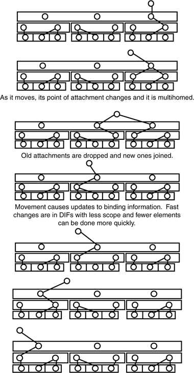
Figure 9-6. As a mobile host or application moves, it joins new DIFs and drops its participation in old ones, at times being multihomed to more than one. The rate of change is commensurate with the scope of the layer. The smaller scope, the faster it may traverse it, and the fewer elements of the layer that need to be notified.
So, while we might like to speak of the addresses associated with mobile systems changing to reflect its new location in the layer, it is more correct to say that a mobile system acquires new addresses and ceases to use old ones. Above the first layer, it will be more important that the addresses assigned indicate where the system is attached to the network. It will also become more important to track the changes in routing and ensure that routing updates are made in a timely manner. Although the number of IPC processes in an (N)-DIF increases with higher layers, the rate of change will decrease. However, it will be advantageous to ensure that nearby systems are updated sooner. And this is precisely the environment we noted for IAP in Chapter 7. In addition, it will also be useful for PDUs in transit to be redirected to different IPC processes. Techniques for this are well understood.
How many layers would a mobile system have? As many as needed. The answer to this question is fundamentally an engineering problem that depends on the size of the network and the rate of new address acquisition. We have seen that the cell phone system performs quite well with two layers and three levels of addressing. But this is based on relatively long new address acquisition rates on the order of minutes and hours. And although it could without doubt perform at a rate of seconds and minutes, a system with a faster address acquisition rate might require more layers to ensure that routing updates could be made in a timely manner.
Will there be a problem with propagating these changes in address throughout the network?
This is the first question that comes to mind. The reason is that there is a tendency to see this as a directory update and to compare it with update times for DNS. This is a not the right view. This is a routing update. The changes only need to be propagated to other IPC processes within the (N)-DIF. The change does not need to be reflected in the (N+1)-DIF (yet) because the (N+1)-DIF is still topologically significant. The lower the layer, the greater the rate at which the binding will change. The higher the layer, the slower the rate of change. This is a direct consequence of the larger scope of higher layers. Changes will be the greatest in those layers with the smallest scope and where the time for the propagation of updates will be the shortest.
Actually, DNS updates are routing updates, too, but that was not understood when DNS was proposed. For mobility, where routing changes occur more frequently, it is important to maintain a balance between the scope of a layer (subnet) (that is, the number of elements that must be updated) and the rate of routing changes. We have seen that a traditional cellular system works reasonably well with three levels of addressing. But if the density of base stations were increased to accommodate more users, or more rapid movement between subnets were required, additional layers might be used so that updates would affect fewer nodes. In fact, given the recursive nature of the architecture, this could lead to a network with a different number of layers in different parts of the network (more in densely used areas, and fewer in less densely used areas).
Isn’t this at odds with the hill and valley model described in Chapter 8? Not at all. Mobile networks by their nature are subnets that are either independent of or at the periphery of a fixed network. In a sense, mobile networks surround the hill and valley model of the fixed network (see Figure 9-7). The common layer that user applications communicate over runs “over the top.” The border between a fixed network and mobile network would meet at the “top of a hill,” just below this common layer. No one incurs any more overhead than required to meet the requirements of the network and the applications.

Remember, too, that these changes are entirely internal to the operation of the distributed IPC facility at that rank. The application names of the user applications and of the IPC processes in all DIFs/layers do not change. However, new instances may be created. This makes it clear why mobility in IP networks is so complicated: With no built-in support for multihoming and not enough names, there is no way to make mobility straightforward. The lack of a complete addressing architecture again takes its toll.
For wireless mobility, we can surmise that each (N)-IPC process will monitor the QoS (signal strength) of its PoAs dropping those that fall below certain parameters and acquiring new ones whose QoS has exceeded some threshold. At the bottom, this will entail frequent enrollments in new lower layers and less frequent enrollments in new higher DIFS. One could view this constant monitoring of the lower-layer QoS with the result that PoAs are dropped as unique to mobility. But this is not the case. It is more common with mobility but not unique. Wireline systems should be (and are) in effect doing the same thing as they monitor the QoS of various PoAs to make decisions about routing. The only difference is that the “failure” rate for wireline systems is generally much lower.
Another major form of mobility that we need to look at is what has come to be called ad hoc networking, where mobile end systems or subnets communicate with other mobile end systems or subnets. Let’s see what the architecture has to say about this and what new problems it might pose.
The operation of a layer in an ad hoc network works in the same way. Each system in the ad hoc network has one or more (1)-layers, one for each wireless channel it can send and receive on. Each (1)-layer is essentially a star topology. Because the physical medium is multiple access, there will be multiple systems participating in this (1)-layer. The constraints on the single wireless channel are such that the (1)-layer will have sufficiently small scope that we can assume a flat address space. As noted earlier, it is an engineering design choice whether the addresses are unambiguous across many instances of a (1)-layer (as with MAC addresses) or only unambiguous within a single (1)-layer, or somewhere in between.
The boundaries of the (1)-layer are determined by the physical medium. The boundaries of higher layers are less constrained and determined by considerations of locality, management, traffic patterns, and so on. Generally, subnets are made up of elements in the same area. Determining such proximity in a truly ad hoc network can be difficult. Reference to an external frame of reference (for example, GPS or the organization of the user) would make it easier. But even with that there is the problem of characterizing and recognizing viable clusters as subnets with truly fluid movement of ad hoc systems. How this could be accommodated would depend on the specific ad hoc network. These are really issues of policy and do not impact the architectural framework. It is sufficient to see that the architecture as developed supports a consistent set of policies. One might, for example, have an ad hoc network with a flat layer address space for all (2)-layers. In this case, systems could join a (2)-DIF as described previously and essentially self-organize into a (2)-DIF. There might be an upper bound on the number of participants and further rules for creating a second one and creating a (3)-DIF for relaying between them and so on.
The further question is this: Can topological addresses be assigned in an ad hoc network? Again, this will to a large degree depend on the specific ad hoc network. Is it large enough that there is an advantage to using topological addresses? Is address acquisition sufficiently constrained or the rate of change sufficiently slow to warrant their use? The Internet makes a good case for large networks without location-dependent addresses, but the constraints of ad hoc networks may argue for smaller subnets. In our development of topological addresses, we found that the topology adopted should be an abstraction of the underlying graph of the network or the desired graph (that is, according to a plan). The same applies to an ad hoc network. The expected deployment may imply a topology. The collected (1)-layers are a set of overlapping star networks, with each system being a center. Clustering algorithms might be used to self-organize higher layers. Again, the rate of change would be a major factor in the practicality of applying such techniques.
Any topology is going to be an abstraction of the relation among the (1)-DIF stars. But the very nature of ad hoc networks is that this relation is fluid. This would seem to imply that these topological addresses are not applicable to purely ad hoc networks (that is, those that have no reference to an external frame of reference). Ad hoc networks with an external frame of reference may be able to use this frame of reference as a basis for a topological structure.
The last case we need to consider is application processes moving from host to host. This problem was actually investigated before the other forms of mobility on the UC Irvine ring network in 1972 (Farber, 1972). Since then, many distributed systems projects have contributed to the problem. Here we are primarily interested in what this model tells us about this form of mobility.
Clearly, the only case that is interesting is applications moving while they are executing. We saw that with recovery that all the state that must be “recovered” is in the application process, not in the IPC or the application protocol, which are stateless. For IPC, there is no difference between a recovered flow and a new flow. The dialog must resume from the last information the application received.
The solution to mobile applications is similar in that we are not so much concerned with moving executing processes as we are with initiating a new instance on another system and then synchronizing state with the existing copy, and then the existing copy can disappear. How might we accomplish this? Consider the following example:
You are in a voice conversation on your computer at your desk. However, you need to leave for another meeting but want to continue the phone call. For the sake of argument, let’s assume that the AP name is a multicast name. Your APM and the APM on the other end are the only members of the multicast group.
To move your phone call, you direct your “cell phone” to join the conversation. The phone creates an instance of the phone conversation APM on your cell phone. The APM joins the AP using the AP name as a multicast name. The phone conversation is now a multicast group consisting of three participants: the person you are talking to, you on your computer, and you on your cell phone. When you are satisfied that the cell phone application is in the call, the APM on your computer can drop out of the call and you can continue to use your cell phone. Or maybe it doesn’t. Perhaps your computer continues to record the conversation for you.
Put simply, mobile applications are just a form of multicast. Very straightforward and, with our simpler approach to multicast, much more easily implemented. One could easily imagine using this with other, more complex applications that were not streaming. In this case, the new APM would join the multicast group, open a separate connection with the primary synchronize state, and then assume the role of the primary or of a hot spare. A nice little trick for applying the model.
But upon reflection, one realizes that this little trick has deeper implications. There is an invariance in the addressing architecture that we had not previously called out: system dependence/independence. Application process names/multicast names are location dependent and system independent; but application PM-ids are location independent and system dependent. This yields a very nice progression:
(N−1)-addresses (PoAs) are location dependent and interface or route dependent.
(N)-addresses (node addresses) are location dependent and interface or route independent.
APM-ids are location independent and system dependent.
AP names are location independent and system independent.
In this chapter, we have looked at the problems of multihoming, mobility, anycast, and multicast; and we have found that all four fit nicely within the NIPCA structure. No new protocols are required. Multihoming and mobility are an inherent part of the structure and can be provided at no additional cost. Multicast and anycast require only the ability within layer management to distribute set definitions and the algorithms for evaluating the set at the time the forwarding table is updated. But more important, we have found that in a recursive structure multicast comes down to what is essentially two cases of unicast. We have also explored the properties of multiplexing multicast groups. This would increase the efficiency of multicast and make its management easier.
All of these are accommodated without special cases, and none of these capabilities was a consideration when we derived the IPC model back in Chapter 6, one more indication that we may be on the right track.
[1] To reiterate, the original justification to build the ARPANET was resource-sharing to reduce the cost of research. However, Baran’s original report and many subsequent arguments to continue the Net appealed to reliability and survivability.
[2] For example, until recently peering for traffic between two Boston area users on different providers took place 500 miles away in Virginia.
[3] There seems to be a penchant among humans to believe that things as they are will remain as they are forever. Even though there is overwhelming evidence that this seldom the case, we still insist on it. Therefore, many argue that the granularity of exchange will remain as it is and not become any finer. An increase in local traffic does not necessarily imply new behavior in the network but can result simply from growth. The decision for more exchanges is driven by absolute cost, not relative numbers. Unless the the growth of the network begins to slow which seems unlikely, if anything there will be orders of magnitude more growth.
[4] This is called the pseudo-header. The necessity of this has been questioned for many years. The rationale given was as protection against misdelivered PDUs.
[5] Some contend that because ASs were originally designed into BGP, it is not a band-aid. ASs are a band-aid on the architecture. Routing is based on addresses carried by PDUs, not by out-of-band control traffic. This has more in common with circuit switching.
[6] This is reminiscent of Needham’s short discussion of irrational numbers in Volume III of Science and Civilization in China. After recounting the problems irrational numbers caused in Western mathematics, Needham turns to China and says, that because China adopted the decimal system so early, it is not clear they ever noticed there was a problem! They simply carried calculations out far enough for what they were doing and lopped off the rest! Ah! Ever practical!
[7] These separate steps are in terms of route calculation to generate the forwarding table, not in forwarding itself. However, this does imply that path calculation (that is, changing the path to the next hop) could be done to update the forwarding table without incurring a route calculation.
[8] Strictly speaking, current algorithms must calculate all the possible routes and then aggregate the common ones. Various workarounds have been introduced to avoid this at the cost of additional complexity. By calculating on node addresses rather than points of attachments, the bulk of the duplication is never generated in the first place.
[9] Unfortunately, most of the literature must be classed as more thesis material than truly concerned with advancing understanding of multicast.
[10] Unicast being the term coined to denote traditional pairwise communications to contrast it with multicast.
[11] The term used in symbolic logic to refer to these two operators. See, for example, Carnap (1958).
[12] They are called anycast “addresses” in the literature, but they are names of sets; and the same arguments we just used to argue that multicast “addresses” are not addresses apply to anycast, too.
[13] Odd that the staid, conservative, old-model telephone carriers could part with tradition, but the innovative, visionary Internet has not been able to.
[14] And because no networking text teaches the principles of network naming and addressing, we are constantly inundated with demands to make IP addresses portable. After all, if the telephone company can, why can’t the Internet. Of course, the answer is that the phone company doesn’t make point-of-attachment addresses or node addresses portable and neither can the Internet. But every few months, some Internet “expert” calls for it.
[15] In the same way that an Ethernet segment constitutes a data link layer, each cell phone tower or wireless base station should be modeled as a single layer. Note how this is reflected in an 802.11 header by having four addresses, two for each layer (one for the base station, and one for the “Ethernet segment” operating over it).