
Chapter 17. Crystallization from Solution
Why study crystallization from solution?
• Many products are sold in solid form, and crystallization is often the last step in manufacturing.
• Crystallization is useful for both nonvolatile and heat-sensitive compounds that cannot be distilled.
• Crystallization often produces very pure products because at equilibrium many crystals are pure.
• Crystallization typically has relatively low energy requirements.
• Crystallization is commonly used to produce inorganic chemicals and pharmaceuticals.
How is crystallization from solution similar to other separation processes, and what is different about crystallization? Crystallization can be designed as an equilibrium-staged system, usually with a single equilibrium stage. In this sense, crystallization is quite similar to extraction and leaching. However, unlike processing gases and liquids, particle size and shape of solids are extremely important. Thus, for a complete crystallization design we must also consider mass transfer, growth kinetics, and crystal size distributions.
Note: A nomenclature list for this chapter is included in the front matter of this book.
17.0 Summary–Objectives
After completing this chapter, you should be able to satisfy following objectives:
1. Do solubility calculations for cooling, evaporation of solvent, addition of antisolvent, and salting out
2. Do yield calculations for different types of crystallizers
3. Use temperature-composition and enthalpy-composition diagrams for binary crystallization calculations
4. Analyze experimental sieve data to determine crystal size distribution (CSD)
5. Explain trade-offs between nucleation and growth in crystallizers
6. Explain assumptions involved in the derivation of the McCabe ΔL law
7. Derive basic population balance
8. Explain mixed-suspension, mixed-product removal (MSMPR) assumptions, and use MSMPR distributions to determine or analyze CSD for continuous crystallizers
9. Analyze CSD of seeded batch crystallizers.
17.1 Basic Principles of Crystallization from Solution
17.1.1 Crystallization Process
A schematic diagram of a crystallization process is shown in Figure 17-1. Solute solubility in solvent depends on the choice of solvent, temperature, and additives. Reasonably high solubility at feed conditions and significantly lower solubility in the crystallizer can lead to a process with high feed capacity and high yield of desired solute. Crystallization requires concentration be greater than the equilibrium solubility (called supersaturated). Methods used to achieve supersaturation of solute include
• Cooling
• Remove solvent (e.g., by evaporation)
• Add antisolvent
• Salting out (add salt)
• A combination of the above
Each of these methods has advantages and disadvantages that are discussed later. The method chosen dictates the type of crystallizer employed.
In addition to a crystallizer, we must have equipment to separate solids from liquid and to do a final purification of solids. Similar to extraction, solvent must be recovered and recycled to have an economical process.
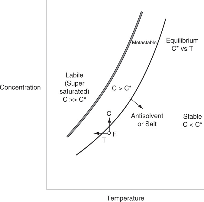
Once the feed solution is saturated, it is sent to the crystallizer where it is supersaturated by cooling, removing solvent, adding antisolvent, or adding salt. To have mass transfer from solution to growing crystals, the solution has to be supersaturated. Most crystallization systems have a metastable region (Figure 17-2) where the solution is supersaturated but few nuclei are formed. The metastable region is a rate effect, not an equilibrium condition. Because downstream processing steps, shown in Figure 17-1, usually function best with large (1 to 3 mm), regularly shaped crystals, nucleation must be controlled. In other words, we want a modest number of nuclei to grow and become relatively large instead of a huge number of nuclei that are stunted and remain small. This situation is analogous to a pond with a huge number of small, stunted pan fish. If there were fewer fish, they would have more to eat and would grow significantly larger. One way to control the number of nuclei is by operating in the metastable region and seeding with a carefully controlled number of small crystals (see Section 17.7). Since crystal growth is quite slow (typically in range of 0.01 to 1.0 mm/h), crystallizers are often very large to provide sufficient residence time.
Continuing with the process description (Figure 17-1), the mixture of solids and liquid (called magma) from the crystallizer is sent to a solid-liquid separator (e.g., a filter, centrifuge, or cyclone). If they are pure enough, wet solids are sent to a dryer that produces the final dry, solid crystals. If a higher purity is required, wet solids may be washed with pure solvent, or further purification may be obtained by dissolving crystals in pure solvent and recrystallizing. Solvent evaporated in the dryer is usually pure enough to be directly recycled to the step (not shown) in which raw feed consisting of solute and impurities is dissolved in solvent.
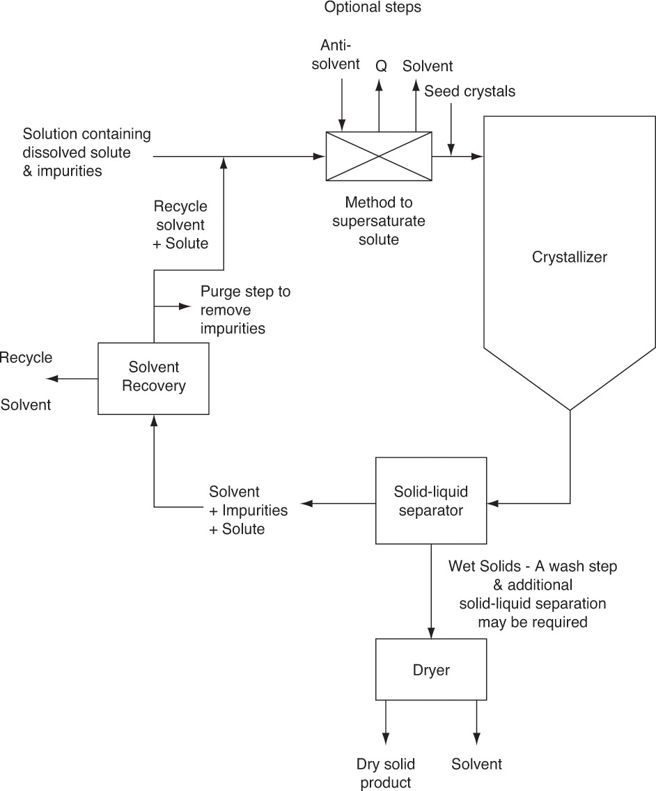
Liquid (called mother liquor) from solid-liquid separation contains solvent that is saturated with solute and impurities. Recycling solute is desirable because it increases yield. However, there must be a method to remove impurities, or they will build up to unacceptably high levels. A separate impurity removal step (e.g., with a membrane system or adsorption) may be required. A purge step (shown in Figure 17-1) may be sufficient to prevent impurity levels from becoming too high. Since purge also results in loss of some solute and solvent, purge is usually employed when initial impurity concentrations are low. After the purge step, solvent plus solute and any remaining impurities are recycled and mixed with fresh feed.
17.1.2 Binary Equilibrium and Crystallizer Types
The Gibbs phase rule for a binary system (e.g., water and a salt) with liquid and solid phases in equilibrium is
degrees of freedom = # components – # phases + 2 = 2 – 2 + 2 = 2.
One degree of freedom is used to set a constant pressure. The second degree of freedom is often used to set system temperature. Once T and p are set, we have no further control over the system at equilibrium. The simplest equilibrium behavior occurs when there is a single solute dissolved in pure solvent and crystals that form are pure solute. Thus a single equilibrium stage is sufficient. We cannot make feed of a particular system at a given concentration follow this behavior. The system may follow this behavior, it may crystalize as a hydrate (next paragraph), it may crystallize out pure solvent (end of this section), it may form eutectics (Section 17.2.2), it may form solid solutions (Section 17.2.2), or it may precipitate as an amorphous mass (Section 17.9).
Figure 17-3 illustrates solubility of aqueous salt systems in concentrations below the eutectic concentration at temperatures above the freezing point of water, and Table 17-1 lists solubility of aqueous solutions of some organic and inorganic materials. We can identify several behaviors in Figures 17-3a and 17-3b. First, many salts, such as NaCl, crystallize as stable anhydrous (no water molecules) crystals within the temperature range of these figures (see Problem 17.F1 for a wider temperature range). Other salts crystallize as stable hydrates. For example, CuSO4·5H2O is a stable solid in range from 0°C to 100°C. Hydrates have a fixed number of moles, n, of water per mole of hydrate. The water of hydration either is bound to the metal or has co-crystallized with salt into a stable crystal form.
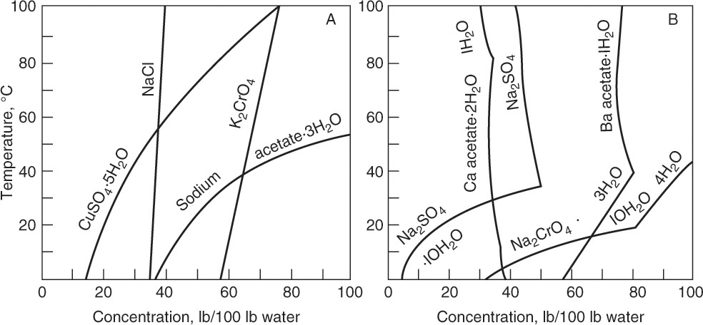
FIGURE 17-3. Solubility diagrams. (A) Systems without crystal phase change. (B) Systems with crystal phase changes. Mullin, J. W., Crystallization, 4th ed., Butterworth-Heinemann, Woburn, MA, 2001. Reprinted with permission of Butterworths.
If hydrate is dissolved in water, there are no discernable hydrate molecules in solution—in fact if CuSO4 dissociates, there are no discernable CuSO4 molecules in solution either. However, when the solubility limit is reached, hydrate will precipitate out. There can also be phase transitions from one stable hydrate form to another (e.g., Na2CrO4·10H2O to Na2CrO4·4H2O) or from a stable hydrate to a stable anhydrous form (e.g., Na2SO4·10H2O to Na2 SO4). These transitions are considered reversible reactions. For example, crystallization of sodium sulfate hydrate can be represented as the reaction
Na2SO4 + 10H2O ↔ Na2SO4·10H2O
The stable form depends on temperature. If hydrate is heated, the water of hydration can be driven off, leaving anhydrous compound. However, if hydrate is the stable form, anhydrous material has to be stored in a totally dry environment or it will rehydrate. The normal humidity of air often causes rehydration. Generally speaking, as temperature increases, fewer or no water molecules occur in stable crystal forms.
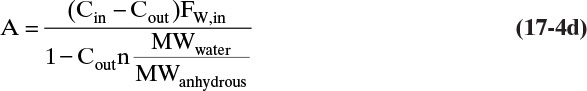
For a general hydrate of the form (anhydrous molecule)·n(water), the molecular weight of the hydrate is
Since there are n moles of water per mole of hydrate, the kg of water of hydration in a hydrate is
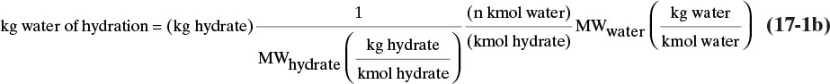
Often we do not carry the units but write this equation as
When a hydrate dissolves in water and forms anhydrous compound and water, we can determine the kg of anhydrous compound from a similar analysis:
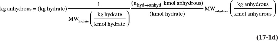
Since there is always 1 mole of anhydrous compound per mole of hydrate, nhyd→anhyd = 1, and when anhydrous compound plus water form hydrate crystals, nanhyd→hydrate = 1. The conversion factor is usually understood, and we write
or
Finally, since nhyd→anhyd = 1, we can calculate the moles of water of hydration for the formation of hydrate from the amount of anhydrous material that reacts:
Table 17-1 is a table of solubilities—not a table of compounds that will be easy to crystallize. Fructose is notably difficult to crystallize and is sometimes added to cake frosting to prevent crystallization of sugars. Data is not presented for fructose at 80°C and 100°C because it decomposes at those temperatures. Data is not presented for sodium acetate·3H2O at 80°C and 100°C because hydrate is not stable at these temperatures.
In solubility tables and figures salt concentration is usually presented as the mass ratio of anhydrous salt (not including any water of hydration) to water. Since there are no permanent hydrate molecules in solution, this convention is logical. Mass balances for salt are done in the same units; thus, salt mass balance ignores water of hydration. Water of hydration is included in water balance. Data is often presented in ratio units, such as kg anhydrous salt/100 kg water (Table 17-1) or moles of anhydrous salt/1000 moles solvent (Figure 17-23).
However, not all presentations and calculations are done in ratio units. For example, for ideal mixtures solubility can be predicted reasonably well from the following equation (Walas, 1985):
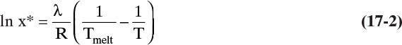
In this equation x* is the mole fraction of solute in solution at saturation, λ is the heat of fusion at the solute’s melting point Tmelt, T is the absolute temperature, and R is the ideal gas constant. Because different units are used, you have to carefully check definitions and units of data.
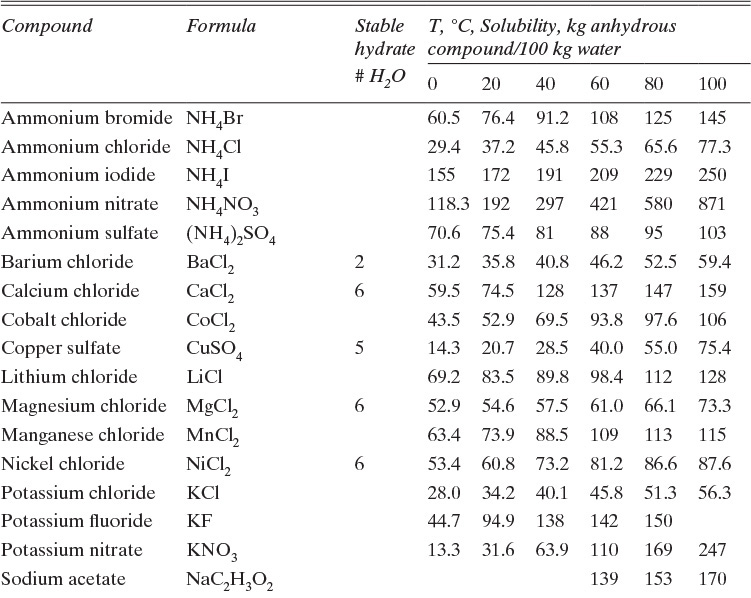
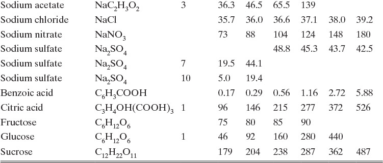
TABLE 17-1. Solubilities of selected inorganic and organic compounds in water (Dean, 1985; Green and Perry, 2008; Mullin, 2001)
The crystallizer type is often dictated by equilibrium behavior. Usually, salts become more soluble as temperature increases, dC/dT > 0, although there are exceptions, such as calcium acetate hydrates (Figure 17-3b). For cooling crystallizers we want a large change in solubility for a small change in temperature, dC/dT >> 0. In Figure 17-2 decreasing temperature T moves the feed point F into the metastable region. In Figure 17-3 sodium acetate and sodium chromate (Na2CrO4) are good targets for cooling crystallizers. For sodium acetate a change from 50°C to 0°C will reduce equilibrium concentration from 100 kg sodium acetate/100 kg water to 38 kg sodium acetate/100 kg water. When cooling crystallizers are discussed in Section 17.2, we will find the data in Table 17-1 is indispensable.
Sodium chloride, on the other hand, is a very poor candidate for a cooling crystallizer. A change of 100°C results in a very small change in solubility of NaCl. Calcium acetate hydrates and anhydrous sodium sulfate do not crystallize in a cooling crystallizer because they become less soluble in water as temperature increases (dC/dT < 0). This reverse solubility as temperature increases can cause problems because these compounds tend to coat and foul heat exchanger surfaces (Moyers and Rousseau, 1987). To crystallize sodium chloride, calcium acetate hydrate, or anhydrous sodium sulfate we would either remove some solvent (C increases in Figure 17-2), add an antisolvent (Sections 17.8.2 and 17.9.1), or add another salt (salting out, Section 17.9.2). Antisolvent and salt additions both change equilibrium behavior and, in Figure 17-2, move the equilibrium curve and metastable region to higher temperatures and lower concentrations. Removal of solvent is often accomplished by evaporation or, if solute is thermally unstable, vacuum evaporation. Evaporative crystallizers are the topic of Section 17.3.
If we have a relatively dilute solution of solute that has a lower concentration than the values listed at 0°C, we can cool the aqueous solution to below the 0°C freezing point of pure water. This freezing point depression depends on solute concentration. If solute is close to saturation and dC/dT > 0 and is relatively large (e.g., glucose at 0.40 kg/kg water), solute will become saturated and crystallize before water freezes. On the other hand, temperature has little effect on solubility of sodium chloride, and if sodium chloride concentration is not close to 0.357 kg/kg water, the freezing point of water will be decreased significantly. The use of salt to prevent water from freezing on highways and sidewalks is common in the United States. However, the story is more complicated than Table 17-1 or Figure 17-3, so we will return to the use of salt to prevent freezing in Section 17.2.2. Many other types of equilibrium behavior occur in crystallization. These different forms are discussed in Sections 17.2.2, 17.3.3, 17.8.2, and 17.9.
17.2 Continuous Cooling Crystallizers
For large-scale production a continuous crystallizer is selected. Batch crystallizers (Section 17.8) are commonly used for smaller production rates. When the equilibrium concentration of solute decreases rapidly as temperature decreases, a cooling crystallizer is effective. Most cooling crystallizers use a heat transfer surface to transfer heat (called indirect cooling). Two major methods are shown in Figure 17-4. The external heat exchanger design (Figure 17-4A) is most common, since it is simple, does not require specialized equipment, and works well for most crystal systems. Crystal product exits in a slurry with mother liquor and has to be sent to a solid-liquid separator (Figure 17-1). The scraped-surface design (Figure 17-4B) is essentially a double-pipe heat exchanger with a rotating scraper cleaning the heat transfer surface. It is useful when crystals adhere to the heat exchanger surface. Continual scraping usually leads to high heat transfer coefficients, but scraping the surface tends to break crystals, making it difficult to grow large crystals. A number of variations of these methods have been employed (e.g., Genck, 1997, 2008; Mersmann, 2001a; Moyers and Rousseau, 1987; Mullin, 2001; and Myerson, 2002).
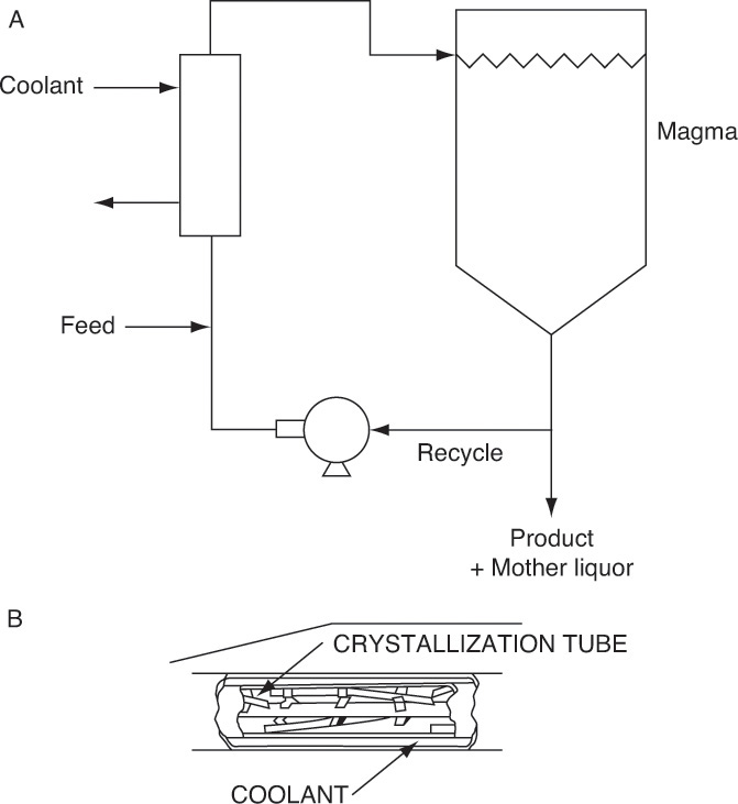
FIGURE 17-4. Continuous cooling crystallizers. (A) Indirect cooling with external heat exchanger. (B) Indirect cooling, scraped surface
Scale-up is difficult for all crystallization equipment. Difficulty arises because turbulence and mixing are different at laboratory, pilot plant, and large industrial scales (Beckmann, 2013; David and Klein, 2001; Tung et al., 2009). These differences mean supersaturation is likely to change during scale-up. Since supersaturation controls nucleation and growth, supposedly similar equipment can behave differently in the plant than in pilot plants or laboratories. In addition to laboratory crystallization studies, scale-up studies are done for new crystallization operations.
17.2.1 Equilibrium and Mass Balances for Single Solute Producing Pure Solute Crystals
Crystallization of a pure, single solute that follows equilibrium behavior discussed in Section 17.1 is important in practice and simple to analyze. Suppose we purify a solute dissolved in a liquid by another separation method such as extraction, a membrane separator (Chapter 18), or adsorption (Chapter 19), but we sell product as a solid. One way to produce product is by crystallization.
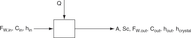
Figure 17-5 shows a very simple schematic diagram for mass balances, and later for the energy balance, on a continuous cooling crystallizer. Since crystallization from aqueous solutions is very common, we assume an aqueous solution is cooled, and operation is at temperatures above water’s freezing point. FW is the water flow rate in kg water/h, A is kg of anhydrous salt in crystals/h, Sc is kg of the stable form (anhydrous or hydrate) of crystals/h, and C is the ratio kg solute/kg water in solution. Following the convention that energy in is positive, Qenergy is the heat load in kJ/s. If the stable crystal form is hydrate, then Sc is kg hydrate/h. If the stable form is anhydrous salt, then Sc = A. The key element in cooling crystallizers is there is no loss of solvent. Development of mass balances is illustrated in Example 17-1 for a system without hydrates and in Example 17-2 for a system with hydrates.
EXAMPLE 17-1. Continuous cooling crystallizer mass balances without hydrates
An aqueous solution containing 1.69 kg potassium nitrate per kg water at 100°C is sent to a continuous cooling crystallizer operating at 40°C. Basis is 100 kg water entering/h.
A. At what temperature do crystals first start to form?
B. How many kg/h of anhydrous crystals are formed?
C. What is the yield of crystals?
Data: From Table 17-1 the stable form of KNO3 is anhydrous, solubility at 80°C is 1.69 kg/kg water and at 40°C is 0.639 kg/kg water.
Solution
A. According to Table 17-1, crystallization will start at 80°C when the solution becomes saturated.
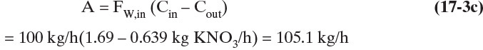
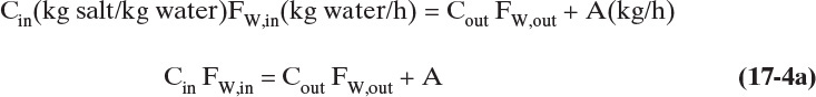
B. Water and KNO3 balances:
and
A is kg/h of anhydrous crystals formed. Solve for A:
C.![]()
and the general equation for the yield in a cooling crystallizer with no hydrates is

EXAMPLE 17-2. Continuous cooling crystallizer mass balances for hydrates
Sodium acetate, NaC2H3O2, saturated at 60°C in water is cooled to 10°C.
A. If salt is dissolved in 100 kg water/h, what are the collection rates of the hydrated crystals and the anhydrous compound?
B. What is the yield of anhydrous compound in crystals?
Data: From Table 17-1 the stable form of sodium acetate at 10°C is hydrate NaC2H3O2·3 H2O. MW anhydrous = 82.04, MW hydrate = 136.09, MW water = 18.016.
Solution
A. Define. We wish to find kg/h of hydrated crystals and the yield of anhydrous crystals.
B. Explore. We can write two steady-state mass balances, one for salt and one for water. Since the inlet solution is saturated with salt at 60°C, concentration can be determined from Table 17-1. We assume outlet liquid is in equilibrium. The value at 10°C can be obtained by linear interpolation in Table 17-1.
C. Plan. Basis: 100 kg water/h entering. Steady-state salt mass balance:
which is identical to Eq. (17-3b). The water balance is different because there is water in hydrated crystals. The steady-state water balance is
The kg of water in sodium acetate hydrate can be determined from the hydrate formula and molecular weights.

In general, 3 is replaced with n mol water/mol anhydrous compound in the hydrate, and the equation is

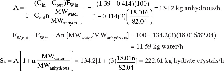
Substituting this result in the water balance gives
FW,in = FW,out + An[MWwater/MWanhydrous]
If we solve for FW,out and substitute in Eq. (17-4a), we can solve for A:
We can also calculate kg/h of solid crystals, Sc, which are the hydrate crystals:
Substituting in Eq. (17-4d), an equation that appears in the literature is

with the molecular weight ratio defined as
Once the kg/s of crystals produced is known, we can calculate magma density, MT, which is the weight of crystals per volume of fluid.
We will discover later that magma density plays an important part in determining crystal size distribution (CSD).
Part B.
D. Do It. Basis: FW,in = 100 kg/h water. From Table 17-1, Cin = 139 kg anhydrous/100 kg water = 1.39 kg anhydrous/kg water, by linear interpolation Cout (10°C) = 41.4 kg anhydrous/100 kg water = 0.414 kg anhydrous/kg water.
Part B. Yield = A/(Cin FW,in) = 134.2/[(1.39 kg anhydrous/kg water)(100 kg water/h)] = 0.965. This is a very high yield. In theory, a cooling crystallizer is a good choice.
E. Check. There are a number of checks that can be run for this problem. First, do calculations agree with an alternate solution approach? The result (see Problem 17.C1) is that the two methods agree. A second check is on parameter values used. Are equilibrium concentrations correct? (As far as can be determined, they are.) Is linear interpolation accurate? This is not a check on numerical calculation but a check on whether the function of the concentration versus the temperature between 0°C and 20°C is linear. Mullin (2001) presents a more complete table that lists equilibrium mass ratio at 10°C as 0.408 kg/kg water. If this value is used to calculate A, the result is A = 134.3. Linear interpolation resulted in a negligible error. Third, there is a practical question: Can we actually run the proposed crystallization in the plant? The answer in this case is probably not. Because slurry is so thick (not enough liquid), mixing and pumping magma is very difficult.
We also want to know how much cooling is required so that we can design heat exchangers. The crystallizer energy balance is
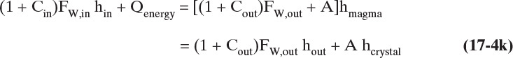
Enthalpy hin is the enthalpy of the feed solution, and hmagma is the enthalpy of the mixed magma. An alternate approach is to split the magma into liquid and crystal phases, which are in equilibrium. The challenge of crystallizer energy balances is obtaining accurate values for the solution and magma enthalpies. Energy balance calculations are considered in detail in Section 17.3.3.
If the stable form of the salt is a hydrate, how do we make up a solution that will be saturated at a given temperature? Adding a hydrate to water adds both salt and water. This question is explored in Example 17-3.
EXAMPLE 17-3. Mixing solutions when hydrates are dissolved in water
The stable form of barium chloride is hydrate BaCl2·2H2O. How do we mix a solution saturated at 100°C with 59.2 kg anhydrous/100 kg water? Specifically, how many kg/h hydrate and water are needed to make 100 kg/h water that is saturated?
Data: MW anhydrous = 208.23, MW hydrate = 244.25
Solution
Let Fhydrate = kg/h hydrate to add and FW,add = kg/h water to add. Then
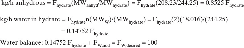
Equilibrium expression: 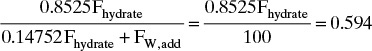
which is, Fhydrate = 59.4/0.8525 = 69.679 kg/h. The general equilibrium expression is
The amount of water to add is FW,add = 100 – 0.14752 Fhydrate = 89.721, and the general equation is
In some cases very little water needs to be added.
17.2.2 Eutectic Systems
There are often limits to solute concentration that result in the formation of pure solute. Figure 17-6 shows solid-liquid equilibrium behavior for a mixture of acetic acid and water at 1.0 atm pressure. This system shows a eutectic, which is very common in aqueous systems. Eutectics are physical mixtures, not compounds. Eutectics are analogous to a minimum boiling azeotrope in distillation. Eutectics freeze with constant composition at a low freezing temperature, while minimum boiling azeotropes boil with constant composition at a low boiling temperature. Binary systems with hydrates often have multiple eutectics.
Eutectics limit crystallization separation in a manner similar to limitation on distillation separation imposed by azeotropes. In Figure 17-6 the eutectic mole fraction is at approximately xAA = 0.31. For feeds with acetic acid mole fractions less than the eutectic concentration, at equilibrium pure ice (a vertical line at xAA = 0) is in equilibrium with the solution shown by the data points. Since temperatures of the liquid and solid are equal at equilibrium, the points in equilibrium are connected by a horizontal tie line. If the feed mole fraction xAA > 0.31, then equilibrium is between the solution and the pure acetic acid crystals (vertical line at xAA = 1.0). A simple eutectic system can produce pure crystals of one compound plus a liquid mixture.
EXAMPLE 17-4. Eutectic equilibrium and mass balances
Determine what happens if we start with 1.0 kmol of a 20 mol% acetic acid, 80% water mixture at 20°C and cool it slowly.
A. At what temperature do crystals first appear? What is the composition of these crystals?
B. At what temperature does the entire mass freeze? At a slightly higher temperature, what two phases are in equilibrium, and what are their compositions?
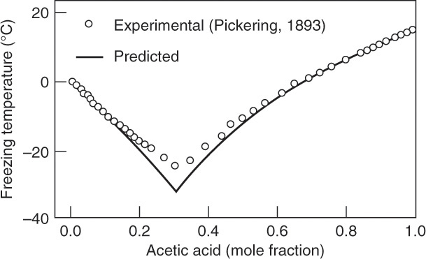
FIGURE 17-6. Binary eutectic system, water-acetic acid. Muir, R. F., and C. S. Howat, III, “Predicting Solid-Liquid Equilibria from Vapor-Liquid Data,” Chemical Engineering, 89 (4), 89 (Feb. 22, 1982). Copyright (c) 1982 Access Intelligence, LLC. Reprinted by permission.
C. What is the yield of pure water in part b?
D. If you want to obtain pure acetic acid crystals, what is the minimum acetic acid concentration of the feed?
Solution
A. From data ∼ –19°C, and from theory ∼ –20°C. Crystals are pure water.
B. If cooled to a eutectic temperature (∼ –25°C according to data; ∼ –33°C according to theory), everything freezes. At a slightly higher temperature, crystals of pure water are in equilibrium with a solution of eutectic concentration, ∼31 mol%. Typically, you should harvest crystals before the eutectic concentration freezes.
C. Feed is 80 mol% water, crystals are pure water, and liquid is 31 mol% acetic acid, which is 69 mol% water.
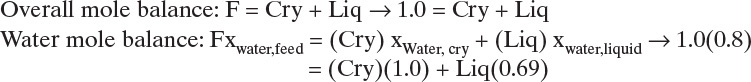
Solving the two equations simultaneously, Cry = 0.3548 kmol, and Liq = 0.6452 kmol.
Yield water = (kmol water in crystals)/(kmol water in feed) = 0.3548/0.8 = 0.444.
D. You can work on only one side of the eutectic at a time. If you want pure acetic acid, you need to start with a feed concentration that is greater than the eutectic concentration of ∼31 mol% acetic acid.
Note: Usually, data are more reliable than theory. The best approach is usually to draw a least-squares correlation through the data, and use the correlation curve to determine concentrations.
Example 17-3 illustrates that with a eutectic system only one pure crystal product can be obtained at a time. Fortunately only one equilibrium stage is needed. Yield is often modest.
The water-sodium chloride mixture used for deicing roads has a eutectic diagram similar to Figure 17-6. The eutectic concentration is 23.3 wt% NaCl, and the eutectic temperature is –21.1°C. If the solution contains less than 23.3% salt, when the solution becomes cold enough, pure water crystals will form. If we add more salt and the mixture is above –21.1°C, the mixture will melt again. However, if we add too much salt, we can pass through the “valley” of the eutectic and form crystals of salt. Crystallization of pure water from seawater (∼3.5 wt% salt) followed by a wash step has been used as a desalination method.
Eutectic diagrams of systems with hydrates can rapidly become rather complicated. This is illustrated in Figure 17-7, a phase diagram for Mn(NO3)2 – H2O (Mullin, 2001). This diagram introduces new concepts of congruent and incongruent melting points. Point B is a eutectic, and between points A and B pure ice is in equilibrium with a solution of Mn(NO3)2 in water. From B to C the solution is in equilibrium with pure Mn(NO3)2·6H2O hydrate crystals. Point C [25.8°C, 62.4 wt% Mn(NO3)2] is a congruent melting point because there is solidification with no change in composition. Point D is a eutectic. Between point D and congruent melting point E [37.1°C, 0.713 mass fraction Mn(NO3)2] the solution is in equilibrium with Mn(NO3)2·4H2O. Between points E and F (another eutectic) the solution is in equilibrium with Mn(NO3)2·4H2O hydrate crystals. From point F to G dihydrate crystals are formed in equilibrium with the solution. Point G is an incongruent melting point (or peritectic point) where dihydrate decomposes reversibly into monohydrate and water, which causes a change in Mn(NO3)2 weight fraction.
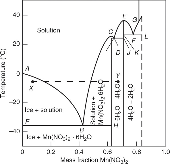
FIGURE 17-7. Phase diagram for Mn(NO3)2 – water. Mullin, J. W., Crystallization, 4th ed., Butterworth-Heinemann, Woburn, MA, 2001. Reprinted with permission of Butterworths.
Mn(NO3)2·2H2O ↔ Mn(NO3)2·H2O + H2O
Figure 17-7 is certainly complicated enough. The good news is that if you were commercially crystallizing an aqueous solution of Mn(NO3)2, you would probably be operating either between points A and B to produce ice and concentrate solution or between points B and C to produce Mn(NO3)2·6H2O crystals. The remainder of the diagram would probably be ignored. The bad news is that Figure 17-7 is considered only moderately complex. For an example of a complicated phase diagram, check out MgSO4 – water (Genck, 2008; Aqueous Solutions Aps, 2015).
There is one additional type of equilibrium behavior that you should be aware of. Except for optical isomers, solid solutions are rare in solution crystallization but fairly common in melt crystallization (Walas, 1985; Wibowo, 2014). In melt crystallization no additional solvent is added and the solvent phase is formed by cooling melt. The y versus x and T versus x-y diagrams for a solid solution have the same shapes as corresponding diagrams for vapor-liquid equilibrium. Figure 17-8a shows solid solution behavior that does not show a maximum or minimum melting point, and Figure 17-8b shows solid solution behavior that shows a minimum melting point (Walas, 1985). Unlike equilibrium discussed earlier, solid solutions require more than one equilibrium stage to obtain a pure or close to pure product. Maximum and minimum melting systems are analogous to azeotropes in distillation. Because multiple stages are required, melt crystallization equipment is very different from equipment used for crystallization from solution. A number of clever ways to obtain pure products by melt crystallization have been developed (Prudich, 2008; Wankat, 1990). Some products purified commercially by melt crystallization include ultra-pure silica and ultra-pure hydrazine; organic acids, including acrylic, benzoic, and carbonic acids; and cyclic compounds, including naphthalene, p-dichlorobenzene, p-nitrochlorobenzene, and toluene diisocyanate (Prudich, 2008).
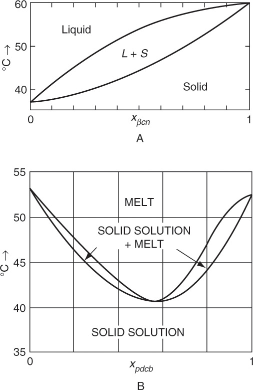
FIGURE 17-8. Phase equilibrium for systems that form solid solutions at 1.0 atm pressure (Walas, 1985). (A)
β-methylnaphthalene + β-chloronaphthalene. xβcn = mole fraction β-chloronaphthalene. (B) p-dichlorobenzene + p-chloroidobenzene. xpdcb = mole fraction p-dichlorobenzene. Walas, S. M., Phase Equilibria in Chemical Engineering, Butter-worths, Boston, 1985. Reprinted with permission of Butterworths.
17.3 Evaporative and Vacuum Crystallizers
Although cooling crystallizers are simple to understand and analyze, many systems have very low crystal yields when a cooling crystallizer is used. Higher yields are obtained when the solvent is evaporated to concentrate the solution to obtain supersaturation. Evaporative and vacuum crystallizers both remove solvent by evaporation. The difference is evaporative crystallizers operate at close to atmospheric pressure and normal boiling points of concentrated solutions, while vacuum crystallizers operate at pressures below atmospheric and thus at temperatures below normal boiling points. Since they operate at lower temperatures, vacuum crystallizers may include cooling. For both methods we assume the solute has a very low vapor pressure and does not evaporate.
17.3.1 Equipment
Equipment for evaporative crystallization is automatically somewhat more complex than for most cooling crystallizers, and vacuum crystallizers add another degree of complexity. Some examples of evaporative crystallizers are shown in Figure 17-9, and vacuum crystallizers are shown in Figure 17-10. A large number of variations of these methods have been invented (e.g., Genck, 1997, 2008; Mersmann, 2001a; Moyers and Rousseau, 1987; Mullin, 2001; and Myerson, 2002).
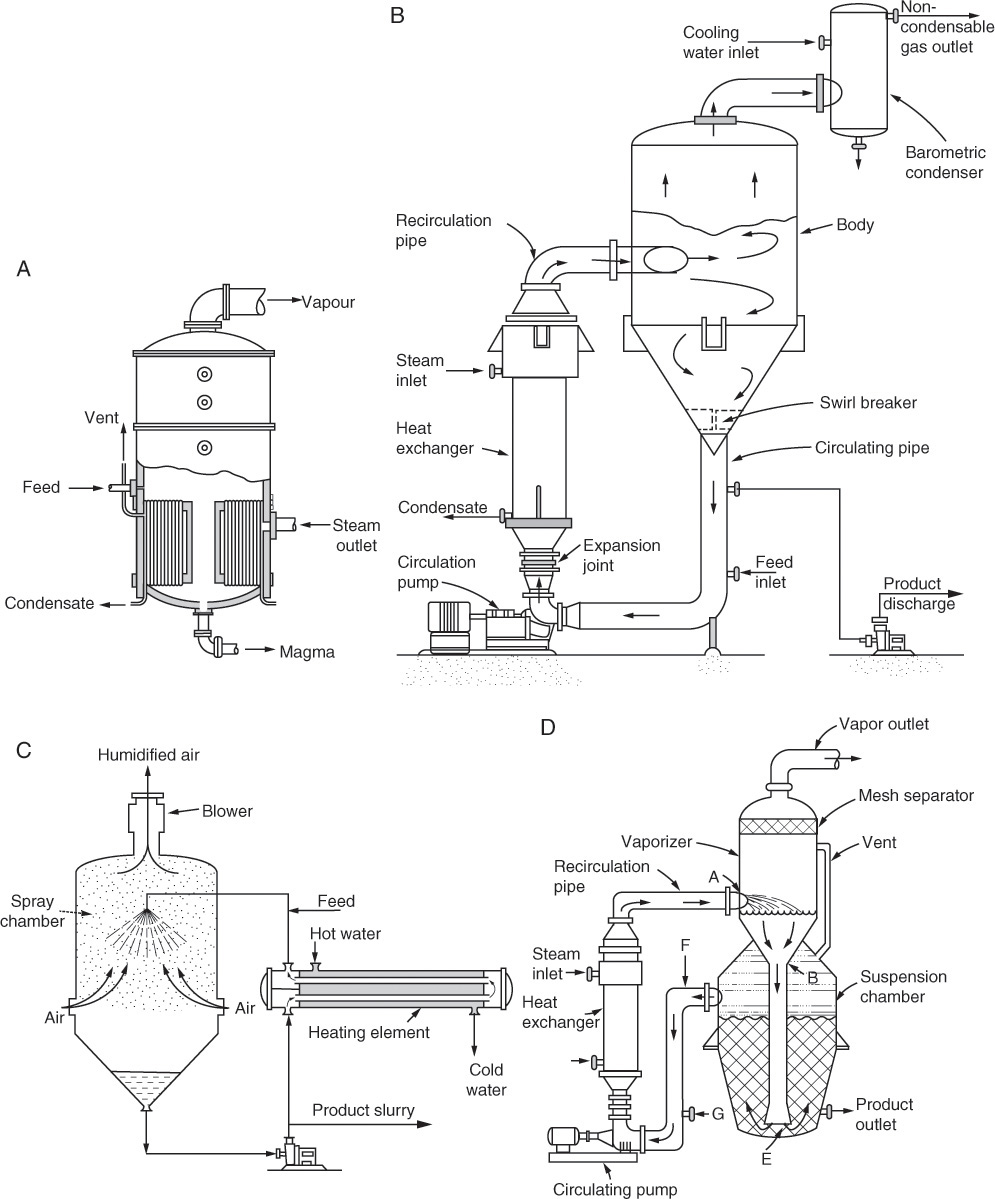
FIGURE 17-9. Evaporative crystallizers: (A) Natural circulation with calandria (Mullin, 2001). Mullin, J. W., Crystallization, 4th ed., Butterworth-Heinemann, Woburn, MA, 2001. Reprinted with permission of Butterworths. (B) Forced circulation-Swenson type (Genck, 2008). Genck, W. J., “Crystallization from Solution,” in Green, D. W., and R. H. Perry, Perry’s Chemical Engineers’ Handbook, 8th Ed., McGraw-Hill, New York, 2008, pp. 18–39 to 18–59. Reprinted with permission. (C) Spray (Bennett, 1988). Bennett, R. C., “Matching Crystallizer to Material,” Chemical Engineering, 95 (8), 118 (May 23, 1988). Copyright (c) 1988. Access Intelligence, LLC. Reprinted by permission. (D) Oslo evaporative crystallizer (Genck, 2008). Genck, W. J., “Crystallization from Solution,” in Green, D. W., and R. H. Perry, Perry’s Chemical Engineers’ Handbook, 8th Ed., McGraw-Hill, New York, 2008, pp. 18-39 to 18-59. Reprinted with permission.
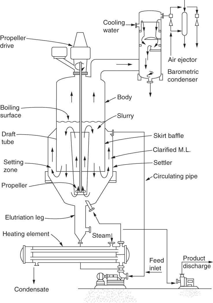
FIGURE 17-10. Vacuum crystallizer. Swenson draft-tube baffled. Genck, W. J., “Crystallization from Solution,” in Green, D. W., and R. H. Perry, Perry’s Chemical Engineers’ Handbook, 8th ed., McGraw-Hill, New York, 2008, pp. 18-39 to 18-59. Reprinted with permission.
17.3.2 Analysis of Evaporative Crystallizers for Single-Solute Systems Producing Pure Solute Crystals
Figure 17-11 is a schematic diagram of a continuous, steady-state, evaporative, or vacuum crystallizer for crystallization of a single solute. This diagram differs from Figure 17-5 only by the addition of vapor stream V. Thus, when equilibrium behavior is in the form discussed in Section 17-1 and operation is above the solvent’s freezing point, calculations are very similar to those in Section 17.2.1. Vapor is assumed to be pure solvent. Since the solvent is often water, in equations and examples we call the solvent water.
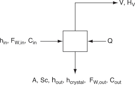
The terms have the same definitions as in Figure 17-5 with the addition V = kg/h of water evaporated and HV = enthalpy of vapor kJ/kg. Example 17-5 illustrates application for an evaporative crystallizer when there are no hydrates, and Example 17-6 illustrates application when there are hydrates.
EXAMPLE 17-5. Evaporative crystallizer without hydrate
A saturated solution of NaCl at 100°C will have water evaporated to obtain a 60% yield of salt. How much water needs to be evaporated for FW,in = 100 kg/h? Data: From Table 17-1 at 100°C, Cin = 39.2 kg/100 kg water.
Solution
Yield = (kg crystals)/(kg salt fed) = A/(FW,inCin). Since the yield is specified, we can solve for A.
A = FW,inCin(Yield) = 100(39.2/100)(0.6) = 23.52 kg/h crystals.
The water balance is
The salt balance is
Solving Eq. (17-6a) for FW,out, substituting it into Eq. (17-6b) and solving for V, we obtain
For the special case of this evaporation in which the temperature remains constant, Cin = Cout, and Eq. (17-6c) simplifies to
Then V = 23.52/0.392 = 60 kg/h.
EXAMPLE 17-6. Evaporative crystallizer with hydrate
A vacuum crystallizer operating at 80°C is used to concentrate and crystallize barium chloride, BaCl2. The feed is saturated at 100°C. For an entering water rate of FW,in = 100 kg/h, V = 40 kg/h of pure water evaporated. Find the values of A and Sc.
Data: The stable form of crystals is BaCl2·2H2O. Solubility at 100°C = 59.4 kg anhydrous/100 kg water, solubility at 80°C = 52.5 kg anhydrous/100 kg water. MWanhyd = 208.23, MWhydrate = 244.25.
Solution
This example is a combination of Examples 17-2 and 17-5. The water balance is

The last term is hydrated water from Eq. (17-4c) with n = 2. The salt balance is
Normally, there is no salt in the vapor and yout = 0. If we solve Eq. (17-7a) for FW,out, substitute that result into Eq. (17-7b), and solve for A, we obtain
The derivation of Eq. (17-7c) is left as an exercise (problem 17.C6). For BaCl2 crystallization Eq. (17-7c) becomes
From Eq. (17-4f) we can determine the kg/h of hydrated crystals, Sc.
Sc = A[1 + n MWwater/MWanhydrous] = (30.69)[1 + 2(18.016/208.23)] = 36.00 kg/h
The energy balance for evaporative and vacuum crystallizers is the energy balance for a cooling crystallizer with a term added for vapor flow.
The term hmagma,out is the enthalpy of magma leaving the crystallizer, kJ/kg. Since pressure has little effect on enthalpies of liquids and solids, hin, hmagma,out, hout, and hcrystal are the same at 1.0 atm and at the pressure of a vacuum crystallizer. However, vapor enthalpy HV is affected by pressure, and data at crystallizer operating pressure are needed. The determination of HV is illustrated in Example 17-7.
17.3.3 Simultaneous Mass, Energy, and Equilibrium Calculations
To calculate energy requirements for vacuum crystallizers we need to do simultaneous mass, energy, and equilibrium calculations. Energy balances require either an enthalpy composition diagram or extensive data on heat capacity of crystals and solutions at different concentrations and latent heats of formation of different hydrates and anhydrous crystals. Data on the latent heat of vaporization of the solvent at low pressures are also required (if the solvent is water, this information is readily available in steam tables (e.g., NIST, 2015).
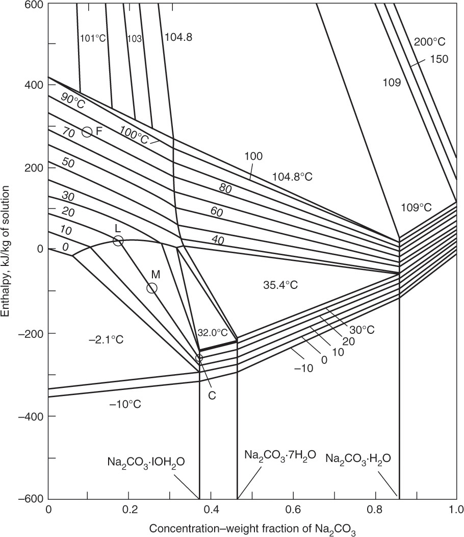
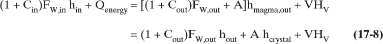
FIGURE 17-12. Enthalpy-composition diagram for Na2CO3 – water at 1.0 atm. Mullin, J. W., Crystallization, 4th ed., Butterworth-Heinemann, Woburn, MA, 2001. Reprinted with permission of Butterworths. Copyright 2001. Points for Example 17-7 have been added.
An example of an enthalpy-composition diagram is shown in Figure 17-12. This diagram looks complicated, but if you understood Figure 2-4 (an enthalpy-composition diagram for ethanol and water), you are well on your way to mastering this diagram.
Figure 17-12 includes all the information needed to solve vacuum crystallizer problems except for the required operating pressure and the enthalpy of pure water vapor at different pressures and temperatures. The required operating pressure can be estimated from partial pressure data for sodium carbonate solutions (Green and Perry, 2008, Table 2-27), and vapor enthalpy is readily available in steam tables (NIST, 2015).
The basis for an enthalpy-composition diagram is the point where enthalpy is arbitrarily set to zero. In Figure 17-12 pure liquid water at 0°C has an enthalpy of zero. This is the same basis used for steam tables, which is convenient, since use of the same basis allows for easy coupling of enthalpy-composition diagrams and steam tables. Use of Figure 17-12 in conjunction with steam tables is illustrated in Example 17-7.
EXAMPLE 17-7. Vacuum crystallizer: Simultaneous mass, energy, and equilibrium calculations
1000 kg/h of a 10 wt% Na2CO3 aqueous feed at 80°C is fed to a vacuum crystallizer operating at 20°C. To concentrate the feed, 600 kg/h vapor is evaporated.
A. What are the compositions of the magma, crystals, and mother liquor?
B. What is the crystallizer pressure?
C. What are the flow rates of the magma, A, Sc, and L?
D. How much energy needs to be removed or added in kJ/h?
Data: Partial pressure of aqueous Na2CO3 at 20°C (Green and Perry, 2008, Table 2-27)

Solution
A. To form concentrated magma, we evaporate vapor from the feed. Overall and sodium carbonate (salt) mass balances with xsalt and ysalt as weight fractions and F total feed flow rate and M total flow rate of magma, both in kg/h, are
Solving for xM,salt and noting that since vapor is pure water, ysalt = 0, we obtain
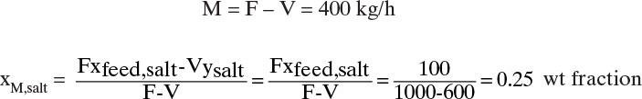
Magma is at 20°C and xM,salt = 0.25. Point M in Figure 11-12 is a mixture of liquid and crystals that split along 20°C isotherm into points L (xL,salt = 0.175) and crystals Cry (Na2CO3·10H2O, xC,salt = 0.370), which are in equilibrium.
B. At 20°C the liquid (point L) is 17.5% salt. Partial pressure data from Perry’s Chemical Engineers’ Handbook at 20°C did not go to this high a salt percentage. We can extrapolate to this value by noting that the change in partial pressure for each 5% change in salt concentration is – 0.3, – 0.4, and – 0.5 mm Hg. If we assume the change is regular, at 20 wt%, partial pressure would be 16.3 – 0.6 = 15.7 mm Hg. Then linearly interpolating to 17.5 wt% salt, partial pressure = 16.0 mm Hg = 2.13 kPa.
C. From part A, M = 400 kg/h. Since concentrations were determined as weight fractions, not weight ratios, we either need to rewrite mass balances or convert weight fractions to weight ratios and then use Eqs. (17-6) and (17-7). Since mass balance in part a is in weight fractions, we will continue on that path. Magma splits into mother liquor with flow rate L and crystals with flow rate Cry, both in kg/h:
Solving for Cry, ![]() . This is the hydrate form (Na2CO3·10H2O), Sc = Cry = 153.8. Liquid flow rate L = M – Cry = 246.2 kg/h. The kg/h of anhydrous crystals is
. This is the hydrate form (Na2CO3·10H2O), Sc = Cry = 153.8. Liquid flow rate L = M – Cry = 246.2 kg/h. The kg/h of anhydrous crystals is
A = Sc (MWanhydrous/MWhydrate) = 153.8(105.99/286.15) = 57.0 kg anhydrous/h
D. The energy balance is
or
Since MhM = LhL + (Cry)hcry, the results from Eqs. (17-10a) and (17-10b) will be identical within the accuracy of the diagram. Thus, from Eq. (17-10a)
From Figure 17-12, hfeed = 283 kJ/kg, hM = –90kJ/kg, and from the steam tables at 2.13 kPa interpolation gives HV = 2534.4 kJ/kg.
Qenergy = 400(–90) + 600(2534.4) – 1000(283) = 1,201,640 kJ/h = 334 kJ/s = 334 kW.
Example 17-7 and Figure 17-12 complete the equilibrium calculations. For a liquid-vapor or liquid-liquid system we completed analyses by determining efficiencies and column diameters. For crystallization we move in a different direction because the size and shape of the crystals is very important. To study size distributions experimentally we can use sieve analysis (Section 17.4). By developing population balances (Section 17.5) we can determine the growth and nucleation parameters from sieve analysis (Section 17.6), and we can predict size distribution once we know growth and nucleation parameters. The required crystallizer volume is determined in the course of this analysis. To control nucleation and grow larger crystals, seeding is often used (Section 17.7). The pharmaceutical industry, a major user of crystallization, employs mainly batch and semibatch crystallizers (Section 17.8) and often employs antisolvents (Section 17.8.2). This chapter closes with a discussion of precipitation and salting out (Section 17.9).
17.4 Sieve Analysis
After we have done a crystallization, how do we determine particle size distribution (PSD) or, specifically for crystals, crystal size distribution (CSD)? A number of electronic devices use laser diffraction, dynamic light scattering, image analysis, electrical zone sensing, x-ray diffraction, and acoustical methods to count particles and determine PSD (Witt and Allen, 2008). An old-fashioned but still commonly used method is to do a sieve analysis (Berglund, 2002; Randolph and Larson, 1988). We describe sieve analysis, since it is the easiest to understand, data analyses for other methods are often similar (Berglund, 2002), and most older crystallization papers report CSD based on sieve analyses.
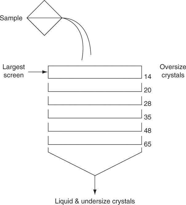
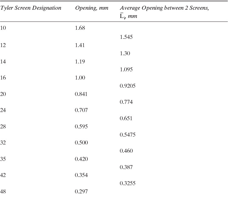
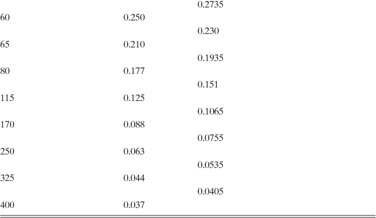
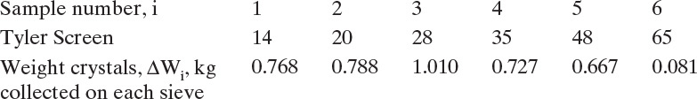
The equipment used for sieve analysis is a series of sieves or screens arranged in a stack with the largest opening sieve on top and the smallest opening sieve at the bottom (Figure 17-13). Sieves are carefully manufactured either as screens with a constant distance between wires or as perforations of constant diameter. Standard Tyler Screen sizes are listed in Table 17-2 (Perry and Green, 1984). The sample is poured into the top screen of the stack while the stack is vibrated. Vibration moves the particles and provides each particle many opportunities to pass through a screen. After sufficient time, the stack is disassembled; crystals retained on each screen are collected, dried, and weighed. Sieve analysis works best when crystals have a fairly uniform shape that is close to cubic. Long, slender crystals often end up being sized by second-largest dimension, not the largest (see Problem 17.A2). Screen analyses are explored in Examples 17-8 and 17-9.
EXAMPLE 17-8. Screen analysis of crystallization data
Screen analysis data using equipment similar to Figure 17-13 were reported for urea crystallization in a commercial evaporative crystallizer (Bennett and Van Buren, 1969). Crystallizer residence time was 3.97 h, and the sample was 10.0 Liter. Urea, C(NH2)2O, is used as a component in fertilizers. Urea crystals were “chunky” (volume = L3, and surface area = 6L2), and their density ρc = 1330 kg/m3.
A. Determine magma density (concentration of crystals in magma), kg/L.
B. Plot the weight distribution (weight of crystals on the screen versus average crystal size ![]() ).
).
C. Plot the number distribution (number of crystals on the screen versus average crystal size ![]() ).
).
D. Comment on what could have been done to improve the data.
E. Define and determine population density, n.
Solution
A. Magma density MT is the weight of crystals per volume, Eq. (17-4f). MT can be determined experimentally by summing crystal weights on all screens to give total sample weight, WT = ∑(ΔWi) = 4.041 kg, and then dividing by sample volume.
Since the sample volume was Vsample = 10.0 L, magma density is 0.404 kg/L = 404 kg/m3.
B, C. The values of ![]() are given for the complete set of screens in Table 17-2. When a standard screen is skipped (e.g., sample 2 includes particles for screen sizes from 14 to 20),
are given for the complete set of screens in Table 17-2. When a standard screen is skipped (e.g., sample 2 includes particles for screen sizes from 14 to 20), ![]() can be calculated from the screen sizes that were used. Thus,
can be calculated from the screen sizes that were used. Thus, ![]() . ΔWi versus
. ΔWi versus ![]() values are shown in Table 17-3. Since the volume of a crystal is
values are shown in Table 17-3. Since the volume of a crystal is ![]() the weight of
the weight of ![]() crystals per volume is
crystals per volume is
and the value of ![]() for each sample is
for each sample is
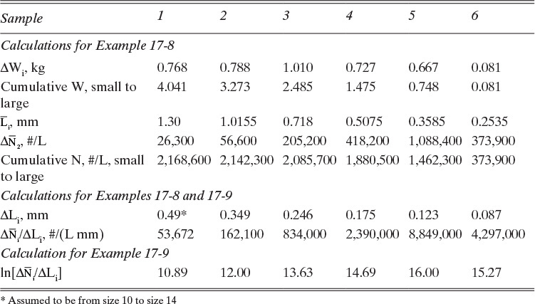
TABLE 17-3. Calculations for Examples 17-8 and 17-9
Since ![]() is in kg and
is in kg and ![]() is in millimeters, it is convenient to determine ρc in kg/(mm)3.
is in millimeters, it is convenient to determine ρc in kg/(mm)3.
ρc = [1330 kg/m3][1 m/1000mm]3 = 1.33 × 10⁻⁶ kg/(mm)3.
Then for sample 2

If we look at cumulative weight (the sum of ΔWi values from the smallest screen [#65] to the current screen) versus crystal length (Figure 17-14), as we go from small to large particles, the weight of the crystals increases. According to theory presented in Section 17.6, we would expect a smooth curve if there were no experimental errors and all assumptions are met. However, as we will see in Figure 17-18, there clearly is some experimental error, and the industrial crystallizer did not meet all assumptions because it was not perfectly mixed.
The cumulative number of particles (Figure 17-15) also increases, but the behavior is different. There are very few large particles, but they increase the length significantly.
D. Since all we know about crystals on the size 14 screen is that they are larger than 1.19 mm, calculations would be more accurate if a size 12 and perhaps a size 10 screen had also been used. In addition, use of a smaller screen (80 or 115 mesh) at the stack bottom would help ensure there were no undersized crystals that were not captured. We can probably assume there were few undersize crystals. However, assuming the large crystals could all pass through a size 12 screen is probably not justified. Thus, we may want to discard the size 14 screen data point for calculations other than magma density. The data would also be improved if there were duplicate points so that error bars could be determined. Measurements of crystallizer concentration would also be useful in later analyses. These points illustrate some of the difficulties in using data from industrial equipment.
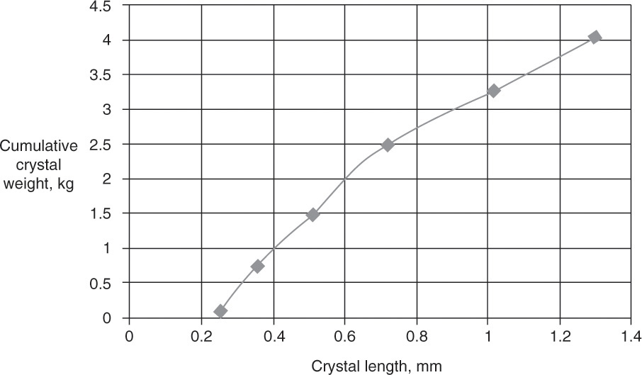
FIGURE 17-14. Experimental cumulative weight versus length determined in Example 17-8
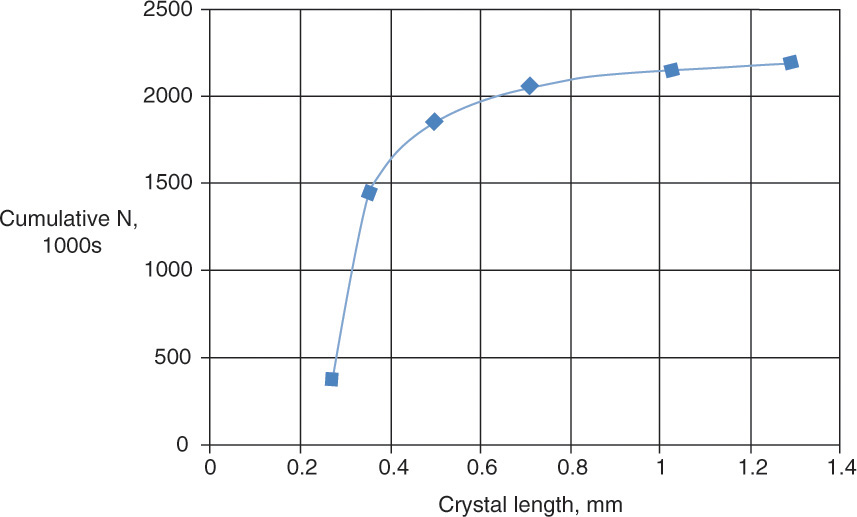
FIGURE 17-15. Example 17-8 results, cumulative N versus length
E. Returning to Table 17-3, ΔLi is the size difference in the two screens used to collect crystals. For example, for sample 2, ΔL2 = Lsize 14 – Lsize 20 = 1.19 – 0.841 = 0.349. We can then calculate ![]() = 56,600/0.349 = 162,100. The interest in this calculation is that in the limit of a very large number of screens (ΔLi → 0),
= 56,600/0.349 = 162,100. The interest in this calculation is that in the limit of a very large number of screens (ΔLi → 0), ![]() , which is the slope of the curve in Figure 17-15 at any specific value of L. Thus,
, which is the slope of the curve in Figure 17-15 at any specific value of L. Thus, ![]() is an estimate of the value of the derivative dN/dL determined at
is an estimate of the value of the derivative dN/dL determined at ![]() . This value is called the population density:
. This value is called the population density:
Classical analyses of crystal size distributions work with population density, which is transformed data, and do not work with raw data (Berglund, 2002).
17.5 Introduction to Population Balances
If we have correct kinetic and mass transfer data, we can predict CSD and the results of a sieve analysis. To do this, we need to introduce population balances. Population balances are a next step up from mass balances. They are not mass balances on steroids but perhaps mass balances on vitamins. Population balances are just a bit more advanced than the mass balances you are familiar with.
Suppose you own a pond, and you are interested in the sizes of all the fish in the pond. You hire an ichthyologist (scientist who studies fish) to examine the fish in the pond. The scientist temporarily stuns the fish (this causes fish no harm) and lays them out in order of size on the edge of the pond. Each fish is marked, and records are kept. The fish are then put back in the pond. Three months later the scientist returns and repeats the process. Suppose you want to know how many fish are in the range of 30 cm to 35 cm. The population balance is
For the fish in the pond, this population balance is
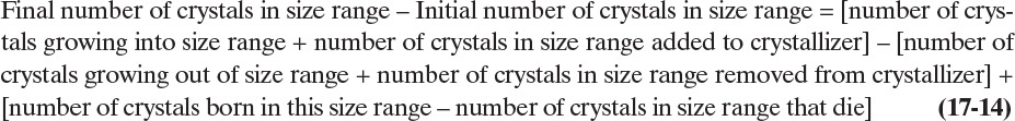
Final number of fish in size range – Initial number of fish in size range = [number of fish growing into size range + number of fish in size range added to pond] – [number of fish growing out of size range + number of fish in size range removed from pond] + [number of fish born in this size range – number of fish in size range that die]
The scientist has measured number of fish in the size range. If you know the average growth rate of the fish, then the number growing into and out of the range can be estimated. Unless the pond is being stocked, no fish this size were added. The number removed would depend on how many people took fish home to eat. Newborn fish are too small to be in this size range. Thus, if the scientist measures the current number of fish in the range, he or she has a very good estimate of the number that died, perhaps by being eaten by other fish.
To study CSDs we can write a very similar population balance. Starting with the general population balance in Eq. (17-13), the population balance for crystals is
Birth and death of crystals occurs when a large crystal is fractured (death of the large crystal) to form two or more smaller crystals (birth of these smaller crystals). Fracturing can occur when crystals are hit by an impeller or when crystals in a scraped-surface crystallizer are scraped from the heat exchanger surface. Birth of a large number of very small particles can also occur when there is micro-attrition of a large particle into a number of small particles, which act as secondary nuclei (Section 17.6), plus a large particle that is slightly reduced in size (Jones, 2002). Birth and death can also occur when there is agglomeration of small particles (death of the small particles) to form a larger particle (birth). Both birth B and death D depend on crystal size.
The number of crystals that will grow into the designated size range depends on the linear growth rate of the crystals, G = dL/dt. Over a time period, Δt, crystals that are within a distance, ΔL = G Δt, of the desired size range will grow into it. Those crystals within ΔL = G Δt of growing out of the desired size range will grow out. The inlet and outlet flow terms depend on volumetric flow rates Q. In symbols the population balance is

Divide this equation by Δt, take the limit as ΔL→0 and Δt→0, and rearrange. The result for a constant-volume system is an unsteady-state population balance:

For a steady-state system, VdN/dt = 0.
Although we could use Eq. (17-15b), it is traditional to write this expression in terms of population density, Eq. (17-12). The constant-volume, unsteady-state population balance becomes

If we assume steady state, ![]() , and the steady-state population balance is
, and the steady-state population balance is
Although Eq. (17-17a) has been simplified, integration for most real systems will need to be done numerically because G is often not constant, density may vary significantly, the crystals do not grow evenly on all faces, the crystallizer is neither well mixed nor plug flow, the kinetics are complicated or unknown, and determination of birth and death functions requires extensive experimental data. However, there is one situation, the mixed suspension, mixed product removal (MSMPR) crystallizer, in which an analytical solution can be obtained. The behavior of MSMPR crystallizers has been extensively studied since many crystallizers follow similar general behavior patterns.
17.6 Crystal Size Distributions for MSMPR Crystallizers
The MSMPR crystallizer is an idealized system that allows us to obtain fairly simple analytical solutions for population density n (Beckmann, 2013; Jones, 2002; Mersmann, 2001b; Myerson and Ginde, 2002; Randolph and Larson, 1988). Once population density is known, the equations for length, area, and mass of crystals can be generated.
To develop MSMPR distributions we assume the following:
1. Constant volume
2. Steady state
3. No crystals in feed, ![]()
4. Product size distribution of product is same as in crystallizer
5. No crystal breakage or agglomeration (which implies B = D = 0)
6. Uniform mixing
7. Uniform supersaturation (c – c*)
8. Mother liquor and crystals in product are in equilibrium (no additional crystal growth in product lines)
9. Constant linear growth rate G
The first three assumptions can be controlled by the operator, and if there are no devices to withdraw particles of different sizes, assumption 4 will often be close to true. Since including birth and death rates of crystals complicates the analysis, the usual initial assumption is that crystal breakage and birth and death rates can be neglected (assumption 5). Uniform mixing (assumption 6) can be achieved in laboratory units and perhaps in pilot scale units but probably is not attained in large, industrial systems. The remaining assumptions are related to uniform mixing and to some extent are contradictory. Uniform mixing is required to have uniform supersaturation (assumption 7), but if mixing and supersaturation are uniform, the product stream cannot be at equilibrium (assumption 8). However, since crystal growth is slow, assumption 8 is not critical. By far the most important simplifying assumption is 9, constant linear growth rate G. To explore the implications of this assumption, we need to take a short detour to look at nucleation and growth.
17.6.1 Crystal Nucleation and Growth
“One of the most difficult processes to scale up successfully is crystallization. Methods to achieve control of nucleation and growth are keys to development, and the degree to which they are successfully applied can be the difference between success and failure in scale-up” (Tung et al., 2009, p. 11).
The kinetic and mass transfer steps for crystal growth are listed in Table 17-4. A given mass of crystals can be obtained with
• Huge number of mainly small crystals—occurs if there is excessive nucleation.
• Small number of mainly large crystals—preferred because downstream liquid-solid separations are simpler (Jones, 2002; Tung et al., 2009).
To obtain large crystals we must control nucleation.
The three main types of nucleation are primary (homogeneous) nucleation, heterogeneous nucleation on foreign objects such as dust particles or irregularities in the crystallizer walls, and secondary nucleation on very small crystals (Mersmann et al., 2001; Myerson and Ginde, 2002; Tung et al., 2009). Since primary nucleation does not occur until a critical super-saturation is passed, it is seldom important in commercial crystallizers. However, since primary nucleation rates become very large at higher values of supersaturation (Figure 17-6), primary nucleation limits the amount of supersaturation that can be used.
2. Bulk diffusion of solvated unit through film
3. Surface diffusion of solvated unit in adsorbed layer
4. Partial or total desolvation
5. Surface diffusion of units to growth sites
6. Move into proper configuration
7. Incorporation into lattice—actual growth of crystal
8. Counter diffusion of solvent through adsorbed layer
9. Counter diffusion of solvent through film
TABLE 17-4. Steps for growth of crystals
Secondary nucleation occurs when tiny crystals of material being crystallized serve as nuclei. The small crystals that serve as nuclei can arise from the breakage of crystal needles or dendrites, from the breakup of agglomerates, and from small crystals formed by contact with a stirrer, a vessel, or other crystals. Collisions that cause secondary nucleation between crystals and impeller, crystals and vessel, and crystals and other crystals occur at approximate ratios of 1000:10:1 (Beckmann, 2013). Coating the impeller and vessel with a soft surface such as a plastic reduces secondary nucleation significantly. Since secondary nucleation depends on collisions and time between collisions increases in large vessels, the rate of secondary nucleation is lower in large vessels.
Heterogeneous nucleation occurs when nuclei form on a foreign object. The most common examples of foreign objects that induce nucleation are dust, small crystallites of a different material from an earlier process (for batch operation) or from an adjacent continuous process, scratches in the vessel, the stirrer, or a purposely added rough object to induce nucleation. Because heterogeneous nucleation probably is not reproducible, it is not good practice to rely on it.
The rate of formation of nuclei, Bo, can often be fit to an empirical power-law relationship (Jones, 2002) that includes magma density MT, stirrer speed Ns, and linear growth rate G:
An energy term may replace the stirrer speed term (Beckmann, 2013). The value of the exponent n in Eq. (17-18) is often close to 1.0 (Beckmann, 2013). For secondary nucleation, i = 0 to 3. This behavior is shown schematically in Figure 17-16. For heterogeneous nucleation, i = 2 to 9. The power-law behavior of heterogeneous nucleation is generally between the curves for primary and for secondary nucleation, as shown in Figure 17-16. In general, to control nucleation we must operate at modest Δc where growth rates are low. Better control of nucleation can be achieved by adding small crystals on purpose as seed crystals (see Section 17.7). The use of seed crystals is widespread in the pharmaceutical industry (Tung et al., 2009).
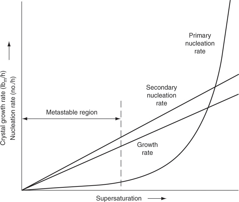
FIGURE 17-16. Qualitative influence of supersaturation on growth and nucleation rates. Supersaturation = Δc = c – c* in kg/m3. Moyers, C. G., Jr., and Rousseau, R. W., “Crystallization Operations,” Chapter 11 in Rousseau, R. W., (Ed.), Handbook of Separation Process Technology, 1987, Wiley-Interscience. Reprinted with permission.
The mass transfer portions of Table 17-4 are illustrated schematically in Figure 17-17. Usually, crystals grow only at specific locations where the energy barrier to incorporating additional molecules is lower. These locations often involve dislocations or steps in crystal structure. Thus, once the solvated molecule reaches the crystal, it still has to migrate to a growth site by surface diffusion as a solvated molecule (step 3) and/or as an unsolvated molecule (step 5) after it is desolvated (step 4), move into the proper configuration (step 6), and then become incorporated into the crystal (step 7). Steps 4, 6, and 7 are kinetic.
Film mass transfer models developed in Section 15.4.1 apply to steps 2 and 9 in Table 17-4.
cI is the interfacial concentration of the solute, kg/m3, and kf is the film mass transfer coefficient, m/h. If the faces of the crystal are growing at the same rate, the mass m of the crystal is
The shape factor is kV = 1 for cubes and kV = π/6 with L replaced by diameter for spheres. The area is
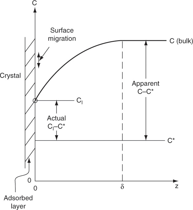
FIGURE 17-17. Mass transfer processes for crystallization. Coordinate z is the distance from the surface of the adsorbed layer.
The shape factor is kA = 6 for cubes and kA = π with L replaced by diameter for spheres. If crystal faces grow at different rates (e.g., platelets or needles), Eqs. (17-19b) and (17-19c) must be replaced by appropriate geometric equations. Shape factors can be difficult to predict since crystals may change shape as they grow.
Surface steps 3 to 8 are usually lumped together and an empirical power-law kinetic model is used.
As always, interfacial concentration cI is difficult to determine. If nr = 1 and kr does not depend on crystal size, we can use a sum-of-resistance model similar to that employed in Section 15.4 to replace cI with the equilibrium concentration c*. This result is

Substituting in Eqs. (17-19b) and (17-19c), we obtain

where k is a combined kinetic and mass transfer constant that is obtained from experiments. Typical supersaturation ratios, c/c*, in crystallizers are from 1.02 to 1.05 (Woods, 2007). If the crystallizer is very well mixed, Δc and hence G will be constant throughout the crystallizer. Integrating Eq. (17-20c) for a well-mixed system, we obtain
Equation (17-20d), the McCabe ΔL law, states linear growth rate does not depend on crystal size (McCabe, 1929). Two salient facts are incorporated in this simple model. First, linear growth rate G depends on supersaturation Δc. Second, many systems at least approximate size-independent linear growth rates. Because a large number of assumptions were made in the model development, experimental justification is needed. However, because it is difficult to achieve perfect mixing in large units, crystal systems that follow Eq. (17-20d) in small-scale units, may not in large units.
If crystal growth depends on crystal size, Eqs. (17-19a) to (17-20d) are not valid. The growth of Na2SO4·10H2O is a well-known example of a crystal that illustrates size-dependent growth with larger crystals growing faster (Abegg et al., 1968). A related problem, growth rate dispersion, is differences in growth rates of individual crystals. Differences occur because not all nuclei are the same shape, and crystal dislocations where growth occurs are different sizes. Fortunately, because the number of growing crystals is very large, measurements in suspensions give a stochastic average that normally compensates for variations (Tung et al., 2009). When Eq. (17-20d) is valid, development of CSD is greatly simplified.
17.6.2 Development of MSMPR Equation and Determination of G and no from Experiment
With the assumptions listed earlier, the steady-state population balance, Eq. (17-17a), simplifies to the MSMPR equation:
where
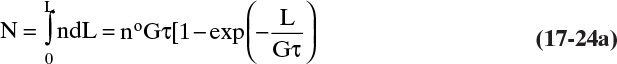
is the retention time. Note that Eqs. (17-21a) and (17-21b) are valid for both cooling and evaporative crystallizers. Equation (17-21a) is an ordinary partial differential equation that can be integrated from L = 0 to an arbitrary length L. The result is the basic equation for MSMPR crystallizers:
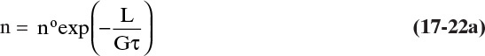
where no, the nuclei population density (value at L = 0), is the constant of integration. The population density is useful because N can be determined by integrating n, N = ∫n dL, and additional useful distributions are easily obtained. Note that no is related to Bo in Eq. (17-18):
If we take the natural logarithm of both sides of Eq. (17-22a) we obtain
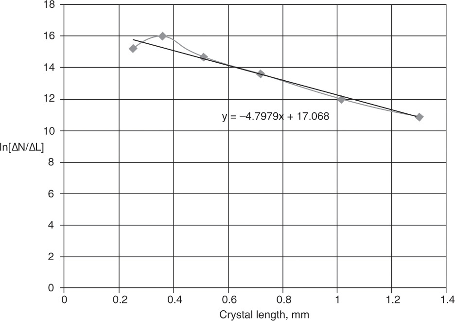
If we have sieve data from a crystallization that approximates the conditions of an MSMPR, a plot of ln n versus L should be a straight line with slope = –1/(Gτ) and y intercept (L = 0) = ln no. Thus the linear growth rate G and the population density of nuclei no can be determined from experimental data. This method is illustrated in Example 17-9.
EXAMPLE 17-9. Determination of kinetic parameters from screen analysis data
Assuming the MSMPR assumptions are approximately valid, determine the linear growth rate constant G and the population density of nuclei no for the crystallization data in Example 17-8.
Solution
Since ![]() is an approximation for n, the MSMPR theory predicts that a plot of
is an approximation for n, the MSMPR theory predicts that a plot of ![]() versus Li will be a straight line. The values of
versus Li will be a straight line. The values of ![]() and
and ![]() were determined in Table 17-3, and the plot is shown in Figure 17-18. Although crystallizers do not always approximately satisfy MSMPR assumptions, the fit is not bad. Slope = –1/(Gτ) = –4.7979. Since τ = 3.97 h, G = 0.0525 mm/h. y intercept = ln[ΔN/ΔL(L = 0)] = ln no = 17.068, → no = 2.585 × 10⁷ # crystals/(L mm).
were determined in Table 17-3, and the plot is shown in Figure 17-18. Although crystallizers do not always approximately satisfy MSMPR assumptions, the fit is not bad. Slope = –1/(Gτ) = –4.7979. Since τ = 3.97 h, G = 0.0525 mm/h. y intercept = ln[ΔN/ΔL(L = 0)] = ln no = 17.068, → no = 2.585 × 10⁷ # crystals/(L mm).
If we discard the data point for the size 14 screen because we do not know the crystal size, we obtain G = 0.05124 mm/h and no = 2.732 × 10⁷ # crystals/(L mm) (see Problem 17.D10).
Note that the two results obtained give an idea of the error. If we know the concentration in the crystallizer c and the equilibrium concentration c*, we can determine the linear kinetic constant k from Eq. (17-19).
17.6.3 Development and Application of Distributions for MSMPR Crystallizers
From 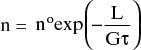 we can calculate physically meaningful distributions. The first distribution of interest is the cumulative number N of particles/volume magma from 0 to L:
The total number of particles per volume is found by integrating from L = 0 to L = ∞:
The dimensionless cumulative number of particles is
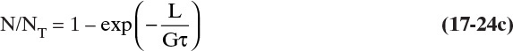
Mathematically, the ratio N/NT is the normalized zeroth moment of the distribution and is shown in Figure 17-19A.
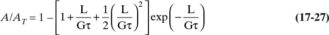
The cumulative length of particles per volume of magma from 0 to L if laid out in a row is

For the total length of all particles per volume, we integrate from L = 0 to L→∞:
The dimensionless cumulative length (the normalized first moment) is

Equation (17-25c) is plotted in Figure 17-19B.
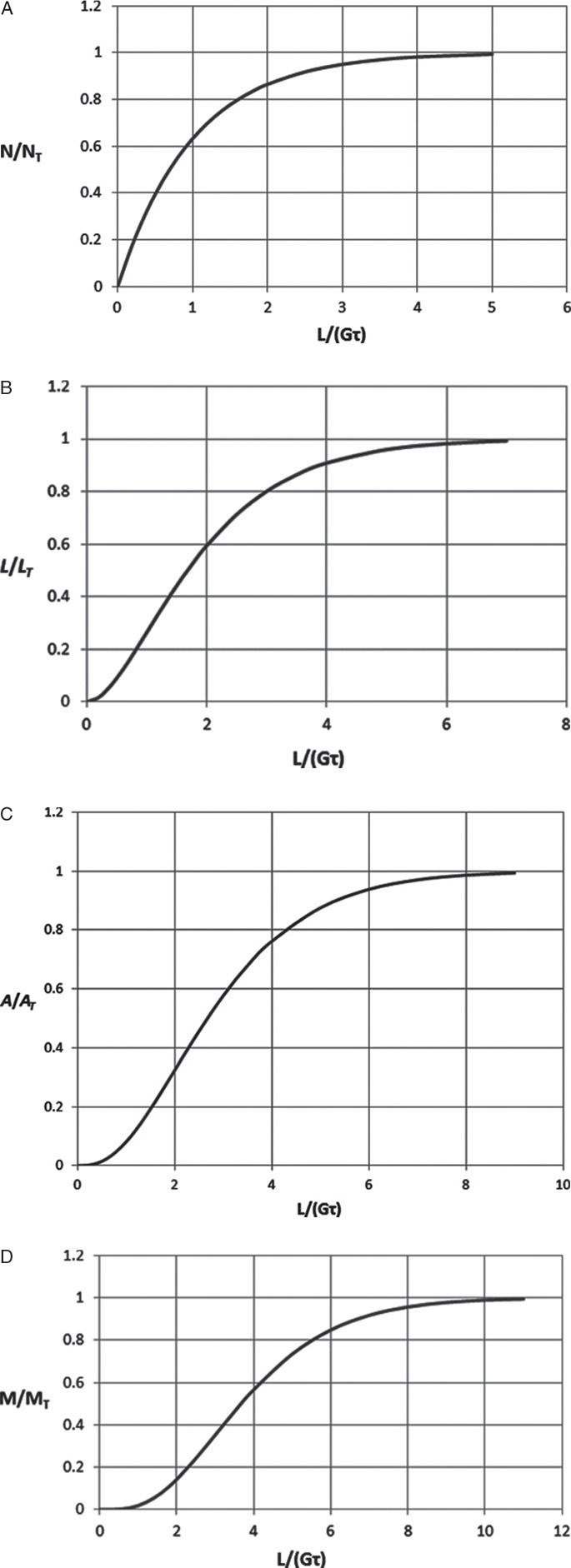
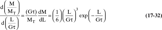
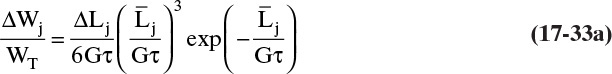
FIGURE 17-19. Dimensionless cumulative distributions for MSMPR crystallizers: (A) number, (B) length, (C) area, (D) mass
The cumulative surface area/volume magma, A, from 0 to L is

The cumulative surface area/volume is useful for mass transfer analyses and can be important in delivery of a drug, since it affects dissolution. The total surface area, AT, of all the crystals is obtained by integrating from L = 0 to L→∞:
Figure 17-19C shows the dimensionless cumulative crystal area/volume (the normalized second moment):
The cumulative crystal volume/volume magma, Vol, from 0 to L is

The total volume of all crystals/volume magma is determined by integrating from L = 0 to L→∞:
The dimensionless distribution Vol/VolT (the normalized third moment) is

If we multiply Vol and VolT by kv ρc the results are the mass M of crystals/volume magma,

and the total mass MT of crystals per volume magma,
The dimensionless distribution M/MT is

Note that this distribution is identical to Eq. (17-28C). Equation (17-30) is plotted in Figure 17-19D. Tables of values of the dimensionless M/MT distribution are available (Randolph and Larson, 1984; Wankat, 1990), but it is probably easier and more accurate to calculate values on a spreadsheet than to interpolate values in a table.
If we compare the distributions when L/(Gτ) = 2.303, we obtain N/NT = 0.9000, L/LT = 0.670, A/AT = 0.405, and M/MT = 0.201. Thus, 90% of the crystals represent 67% of the cumulative length, 40.5% of the cumulative area, and only 20.1% of the cumulative mass. Another way to state this is the largest 10% of the crystals are almost 80% of the total mass.
The weighted average crystal length = 3.67 Gτ is a handy measure of the crystal size. Most industrial crystallizers aim for crystals that are generally of cubic or spherical shape with a diameter or length in the range 0.075 to 3.0 mm, with 1.0 to 1.5 mm being most common (Woods, 2007).
Sometimes it is more convenient to work in differential terms (e.g., amount in each sieve) instead of cumulative distributions. A differential mass distribution is derived by differentiating Eq. (17-28).

For size-independent growth, MT is independent of L. Thus, we can calculate the dimensionless differential mass distribution by multiplying Eq. (17-31) by (Gτ)/MT.
At this point, you have read the pages of equations, but have you tried to do any of the derivations? You can own the equations by deriving them for yourself. Do at least one part of problem 17.C2.
The use of the distributions is illustrated in Examples 17-10 to 17-12.
EXAMPLE 17-10. Use of differential mass distribution to analyze screen analysis data
Use the dimensionless differential mass distribution to analyze the screen analysis data presented in Example 17-8 to determine G and no.
Solution
In terms of experimental values Eq. (17-32) can be written as
In this equation ΔWj is the mass of crystals collected on each sieve j, WT = experimental total weight of crystals = 4.041 kg, ΔLj is the difference between the sizes of the sieve openings of two adjacent sieves,
and ![]() is the mean size of crystals on sieve j
is the mean size of crystals on sieve j
For example, for sample 4 in Table 17-3, τ = 3.97 h, ![]() , ΔW4/WT = 0.180, and ΔL4 = 0.175 mm. Solve Eq. (17-33a) for G for each sample. For example, from Goal Seek on Excel, we obtain G4 = 0.0519. Repeat this calculation for each sample:
, ΔW4/WT = 0.180, and ΔL4 = 0.175 mm. Solve Eq. (17-33a) for G for each sample. For example, from Goal Seek on Excel, we obtain G4 = 0.0519. Repeat this calculation for each sample:

Clearly there is a fair amount of scatter in the results. We can weigh the results by the mass of crystals collected on each sieve and find a weighted average G,
which is Gavg = 0.04936. An estimate of no can be made from Eq. (17-29), no = 3.43 × 10⁷ #/(L mm). Compared to the results from Figure 17-18 [G = 0.0525 mm/h and no = 2.585 × 10⁷ # crystals/(L mm)], the differential approach has a lower value of G, which causes no to be higher. These rates are considered a bit low in industrial applications, since typical growth rates are 0.1 to 0.8 mm/h (Woods, 2007).
EXAMPLE 17-11. Prediction of sieve analysis
Another evaporative crystallization of urea gave: G = 0.0240 mm/h, τ = 6.70 h, no = 9.390 × 10⁷ #/(L mm), kv = 1.0, and ρcrystal = 1.33 g/ml. Suppose we screened a sample of 1.0 L of magma and collected crystals between sieves with Tyler mesh 20 (0.841 mm) and 24 (0.707 mm).
A. Predict the weight of crystals collected between these two sieves.
B. What is the median size (on a weight basis) of distribution? If all of the screens listed in Table 17-2 are used, between what screens will the median size be collected?
Solution
A. MT = 6kvρcno(Gτ)4 = 6(1.0)[1.33 × 10⁻³ g/(mm)3][9.390 × 107 #/(L mm)] × [0.0240mm/h)(6.70h]4 = 501g/L
Note that a conversion for ρc was done to have correct units.
For a size 24 screen, L/(Gτ) = 0.707 mm/[(0.0240 mm/h)(6.70 h)] = 4.397.
From a spreadsheet, we calculate

For a size 20 screen, L/(Gτ) = 0.841 mm/[(0.0240 mm/h)(6.70 h)] = 5.230. Spreadsheet results: M/MT = 0.7658 and M = 383.667 g/L.
Between the two screens, ΔM = M20 – M24 = 383.666 – 320.634 = 63.033 g/L. Since sample was 1.0 L, we predict that we will collect 63.033 g.
This calculation could easily be repeated for each pair of screens to predict the complete screen analysis (see Problem 17.D12).
B. Median size = 3.67 Gτ = 0.590 mm. From Table 17-2, this size would be collected between Tyler meshes 28 and 32.
Crystallization interactions are complex. In Example 17-8 we look at interactions of equilibrium, nucleation, and growth in a cooling crystallizer. After that example, we look at how interactions affect crystal size.
EXAMPLE 17-12. Combination of equilibrium and MSMPR distribution
A cooling crystallizer is crystallizing potassium chloride, KCl, from an aqueous solution at 32°C and 1.013 bar. Feed to the crystallizer is initially saturated at 80°C and is cooled to 32°C. The crystallizer holds 1.5 m3 of magma. We desire a weighted average crystal length = 3.67 Gτ = 1.40 mm. Mullin (2001) reports KCl growth is size independent. Assume the crystallizer can be modeled as an MSMPR crystallizer. Determine the feed rate of the total solution, F kg/h. Data: Garside and Shah (1980) report nuclei population density at 32°C is given by
MT is in kg/m3, and G is in m/s.
Density of solutions: see Table 2-76 (Perry and Green, 2008). kv = 1.0. Crystal form is anhydrous. KCl solubilities from Table 17-1: at 80°C, 51.1 g/100 g water; at 40°C, 40.0 g/100 g water. KCl solubility at 30°C (Mullin, 2001), 37.0 g/100 g water.
Solution
A. Define. Find the feed rate that gives the mean size of mass distribution = 1.40 mm.
B. Explore. At first glance this problem may appear to be impossible, but remember step zero of the problem-solving approach: “I want to, and I can.” If we assume the crystallizer is at equilibrium, we can find the outlet concentration of KCl. Let’s list the equations and see if there is light at the end of the tunnel. For an equilibrium system:
Crystal flow rate for anhydrous crystals = Sc = (Cin – Cout)FW,in
where FW = water flow rate, kg/h; C = kg salt /kg water.
Mass balance: FW,in = F/(1 + Cin)
where F = feed flow rate in kg/h. Since this is a cooling crystallizer with no evaporation of the solvent, Fout = F, and since there are no hydrates, FW,in = FW,out. Volumetric flow rate Qout = Fout/ρ, which is Qout = Fout/ρfeed if we assume constant density or more accurately Qout = Fout/ρprod. For an MSMPR crystallizer: τ = volume crystallizer/Qout, and MT is given by Eq. (17-29), MT = 6kvρcno(Gτ)4. In addition, MT can be determined from equilibrium Eq. (17-4i), MT = Sc/Qout. Median size mass distribution Lmedian = 3.67 Gτ. For KCl at 32°C use Eq. (17-34) to relate no to MT and G.
C. Plan. First use equilibrium data to calculate Cin and Cout. Then calculate solution density. If we guess a value for F, we can calculate FW,in Q, Sc = (Cin – Cout)FW,in, MT = Sc/Qout, and τ = V/Qout. Next solve Eqs. (17-34) and (17-29) simultaneously for G and no.
Solve Eq. (17-29): no = MT/[6kvρc(Gτ)4], and substitute into Eq. (17-34), MT/[6kvρc(Gτ)4] = 7.17 × 1039 MT0.14G3.99.
Solve for G: G7.99 = MT/[6kvρc(7.17 × 1039 MT0.14τ4)] or G = {MT/[6kvρc/(7.17 × 1039 MT0.14τ4)]}1/7.99.
Calculate Lmedian.
Check: Does Lmedian = 1.40 mm (0.0014 m)? If not, pick a new value of F and repeat.
D. Do it. For Cout use linear interpolation to find the concentration at 32°C:

Density of feed solution = 1208 kg/m3, and density of product ∼1181 kg/m3 (calculation of density requires an interpolation of densities to find the density at 32°C and then an extrapolation to the saturation conditions [Table 2-76, Perry and Green, 2008]).
The remaining equations are done on a spreadsheet (in this chapter’s appendix, Figure 17-A1). Convergence is obtained by using Goal Seek to force 1,000,000 * (Lmedian, specified – Lmedian, calculated) → 0 by changing the guessed value for feed rate F. (The multiplier 1,000,000 is used to trick Goal Seek to converge to very small values, since Lmedian is 0.0014 m.) We work in consistent units of kilograms, meters, and seconds and then convert the answer to hours if desired. If we assume that density is constant and use ρ = 1208 kg/m3, the results are F = 1224.99 kg/h, τ = 1.480 h, Sc = 109.36 kg/h, MT = 107.93 kg/m3, G = 7.1578 × 10⁻⁸m/s, no = 4.273 × 10¹¹ #/(L m) = 4.273 × 10⁸ #/(L mm).
If we use the more accurate ρout = 1181 kg/m3, we obtain F = 1190.8 kg/h, τ = 1.488 h, Sc = 106.39 kg/h, MT = 105.52 kg/m3, G = 7.123 × 10⁻⁸ m/s, no = 4.177 × 10¹¹ #/(L m) = 4.177 × 10⁸ #/(L mm). The spreadsheet in Figure 17-A1 shows the solution with ρout = 1181 kg/m3.
E. An exact check is difficult. However, note that G is within the range of validity of the nucleation equation (2 to 12 × 10–8 m/s), and MT is also within the range of validity (60 to 250 kg/m3), as reported by Garside and Shah (1980). Estimation of the outlet solution density is not totally accurate; however, this calculation is more accurate than assuming a constant density equal to feed density.
F. Generalization. The guess-and-check procedure used for this problem is very powerful, but there has to be a check variable. In this case median particle size was specified, and it could be calculated. The check was in agreement between the specified and the calculated mean particle sizes. The assumption of constant liquid density, which is off by 2.2%, caused a 2.8% difference in the feed flow rate compared to the calculation based on estimated outlet solution density.
This example illustrates that equilibrium and population balance are coupled. A number of interactions and feedback loops occur in crystallizers (Berglund, 2002; Genck, 1997; Mullin, 2001). Fortunately, the spreadsheet developed for this example (in this chapter’s appendix, Figure 17.A-1) automatically includes these feedback loops in the calculation. However, you will find working your way through Figure 17-20 to understand feedback loops will be very useful as you solve problems.
Figure 17-20 and the spreadsheet in Figure 17-A1 help to explain how close coupling of nucleation and growth rate makes it difficult to increase crystal size without increasing residence time, τ = V/Q. For example, if we want a 10% increase in median size to 1.54 mm with a constant volume, the spreadsheet result is that feed rate is reduced to 1011.32 kg/h (17.4% decrease in throughput). Population density no is reduced by 31.7% to 2.918 × 10¹¹ #/(m L), which is what allows us to produce larger crystals, but G is reduced to 6.506 × 10⁻⁸ m/s, which is one reason we need a longer residence time.
Equation (17-29) would make us believe that increasing τ will probably increase MT. However, for an anhydrous product Eq. (17-4g) becomes

Substituting this result into Eq. (17-35a), we find

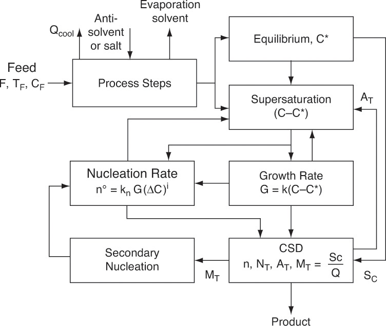
Because equilibrium is not affected by flow rates, magma density MT, which is an intensive quantity, is not affected by the flow rate. Thus, according to Eq. (17-29), quantity noG4τ4 = constant. Since τ was increased to increase crystal size, noG4 must decrease. For KCl nucleation kinetics, Eq. (17-34) in Example 17-12, no decreases significantly if G decreases. For G to decrease, supersaturation (c – c*) has to drop. With a lot fewer nuclei, growth is slower and occurs on fewer crystals; consequently, the crystals become larger. Because all steps are coupled (Figure 17-20), our initial intuition may be wrong.
In Example 17-12 yield (fraction of KCl in feed that becomes crystal product) is
Yield = (Sc)/(FW,inCin) = (Sc)/[(FCin)/(1 + Cin)] = (Sc)(1 + Cin)/(FCin) = 0.2642
which is quite low. Yield, unlike crystal size, is controlled by equilibrium. Yield can be increased by operating crystallizer at a lower temperature, which will decrease Cout and increase yield. A better alternative for KCl crystallization is to switch to an evaporative crystallizer. Increasing the yield is certainly worthwhile. However, there are costs. To operate at a colder temperature more cooling is needed, and since growth rate will decrease, a longer residence time is required to produce large crystals. Nucleation rate also decreases, and that makes producing large crystals feasible only if one is willing to operate with a longer residence time. Costs of an evaporative crystallizer are in the use of a more expensive design and the cost of energy to evaporate solvent.
Obviously, MSMPR theory can be used to explore a number of other scenarios. Some of these scenarios are explored in the problems at the end of this chapter. There are also a number of equipment modifications, such as fines removal and classified product removal, that can be explored with population balances (Jones, 2002; Randolph and Larson, 1988; Wankat, 1990). In addition, somewhat more advanced topics, such as analyzing systems that have size-dependent growth, can be analyzed with population balances (Abegg et al., 1968; Jones, 2002; Randolph and Larson, 1988; Wankat, 1990). If we can disconnect nucleation and growth rates, then we can grow larger crystals with reasonable residence time. The method for doing this, which is extensively used in industry, is seeding (Tung et al., 2009). Since we have covered the basics, you have the necessary tools to tackle these topics.
17.7 Seeding
Seeding is purposely adding small crystals to the feed to serve as nuclei. Seeding reduces the size of metastable region and can provide the desired number of nuclei with a supersaturation level that gives good growth but does not flood the crystallizer with nuclei. If seeds are tightly classified, seeding can give a tighter CSD. In continuous crystallizers, continuous seeding tends to make operation more stable and reduces oscillations (Genck, 1997). Seeding is also common in batch systems (Section 17.8). Most pharmaceutical crystallizers are seeded batch systems.
Seeding is very useful for polymorphic crystals. Polymorphs are crystals of the same molecular species but with different three-dimensional structures. For example, graphite and diamond are polymorphs of carbon. Since polymorphs in pharmaceutical applications have different bioavailability, it is critical to produce the desired polymorph. The thermodynamically most stable polymorph may change when temperature or other conditions are changed. Seeding provides a template so that crystals with the desired three-dimensional structure are more likely to be produced.
Seeding can also provide selective nucleation for fractional crystallization for a system supersaturated with two or more solutes (Tung et al., 2009). For example, since optical isomers have different pharmaceutical properties, they must be separated. Fractional crystallization is one method for doing this separation (chromatography is also used for separating optical isomers); however, fractional crystallization is an advanced topic that is beyond the scope of this chapter.
17.7.1 CSD Analysis for Growth on Seeds in Continuous Crystallizers
Since seeded crystallizers do not meet assumptions made for MSMPR crystallizers, a different analysis procedure is used to develop CSD. First, equilibrium calculations are done following standard procedures. When seeds are added, magma density becomes
WS is the rate at which seeds are added, kg/h.
To develop CSD when seeding is used, assume:
1. No additional nucleation, and seeds do not dissolve in solution; thus, the number of crystals/volume is constant.
2. Assume size-independent growth and Eq. (17-20d) becomes
ΔLgrowth = GΔt = Gτ
Thus, ΔLgrowth is the same for all particles. The ΔLgrowth law was first developed by McCabe (1929) while developing a model for growth on seeds.
3. Seeds have a known CSD. Depending on the method used to measure CSD, distribution could be based on the number of crystals, length of crystals, area of crystals, or weight of crystals. If the known distribution is a weight distribution, then WS and WS,i/WS are known.
4. Since there is no nucleation, the number of crystals in a cohort of seed distribution = the number in the same cohort of product distribution. A constant number of crystals allows for relating seed mass to product mass. If there is equal growth on all three faces,
where ΔWs,i and ΔWp,i are the weight ranges of a cohort in the seed and product distributions, respectively. Since we are interested in the product, solve for ΔWp,i:
Since CSD of the seeds is assumed to be known, once we know the correct ΔLgrowth, Eq. (17-38a) gives the product CSD, and the total weight of the product crystals is
However, since crystallizers must also satisfy equilibrium, which specifies the value of Sc, the crystal product rates are automatically
Thus, we cannot use an arbitrary value for ΔLgrowth. To find the product CSD, pick a value for ΔLgrowth, calculate Wp from Eq. (17-38b), check to see if Eq. (17-39) is satisfied, and if not, try another value. This procedure is relatively easy to do with a spreadsheet and Goal Seek (see Example 17-9).
Note: Individual, larger seed particles gain more mass, but for the same weight of seeds, there are many more small seed particles. The net result is an increase in the relative weight of cohorts of smaller seed crystals.
5. Once ΔLgrowth has been calculated, we need to determine how to achieve the desired growth. Since ΔLgrowth = Gτ, we can usually obtain the desired value of ΔLgrowth by adjusting G (change ΔC) or τ = V/Qout (change crystallizer volume or volumetric flow rate). Since seeding replaces the usual nucleation process, there is considerably more flexibility to change ΔC and τ than in a crystallizer that is not seeded.
Figure 17-21 illustrates feedback loops in a seeded crystallizer with no additional nucleation. The entire system of feedback loops built around nucleation (Figure 17-20) has disappeared. Thus, within limits, supersaturation can be increased to increase growth rate.
EXAMPLE 17-13. CSD of seeded crystallizer
A saturated aqueous solution of sodium acetate NaC2H3O2 at 40°C is cooled to 0°C and fed to a continuous crystallizer. For each 100 kg of entering water, 2.5 kg of hydrated seed crystals are added. The seeds are very tightly classified and can be considered to consist of three sizes, 30% by weight 0.13 mm, 40% by weight 0.15 mm, and 30% by weight 0.17 mm.
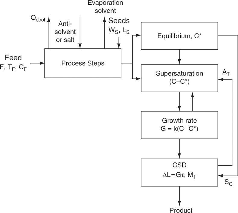
Data: From Table 17-1 the stable form of sodium acetate crystals at 0°C is hydrate NaC2H3O2·3H2O, and solubilities are (in g anhydrous NaC2H3O2 per 100 g water) 65.5 at 40°C, 36.3 at 0°C. ρhydrate = 1450 kg/m3, kv = 1.0.
A. Find kg/h of hydrate and anhydrous products per 100 kg/h of water feed.
B. Find the weighted average size of product.
C. If τ = 19 h, find the linear growth rate required.
Solution
A. Determining the weights of hydrated and anhydrous crystals produced is an application of equilibrium. The only difference between this calculation and calculations in Section 17.2.1 is the weight of the hydrated seed crystals must be added to the calculated value of Sc.
Basis: 100 kg water/h. Thus, WS = 2.5 kg/h. From Eq. (17-4g) for hydrates mass of crystals per hour is

Molecular weight ratio is defined in Eq. (17-4e), MWratio = MWhydrate /MWanhydrous.
The product is NaC2H3O2·3H2O, which has MWhydrate = 136.09, MWanhydrous = 82.04, and the MWratio = 136.09/82.04 = 1.66. Equilibrium data are given in the problem statement. Then, the weight of hydrated crystals produced (not including the weight of the seed crystals) is
Sc = (1.66)(0.655 – 0.363)(100)/[1 – 0.363(1.66 – 1)] = 63.7 kg/h.
Total weight of hydrated product is
Wp = Sc + WS = 63.7 + 2.5 = 66.2 kg/h
and the weight of anhydrous product is
A, kg anhydrous = Wp(MWanhydrous/MWhydrate) = 66.2/1.66 = 39.9 kg/h
B. Assume equal growth in all directions. Basis is still 100 kg/h of entering water. Then 2.5 kg/h of seeds with distribution given in the problem statement are added. Since we calculated Wp = 66.2 kg/h, Eq. (17-38b) is
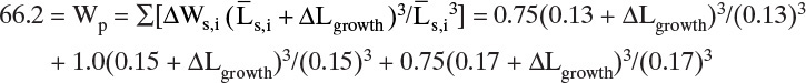
This equation was programmed in a spreadsheet, and Goal Seek was used to find ΔLgrowth = 0.2918 mm (Figure 17-A2). The seeds that were originally 0.13 mm grew to
Lp,1 = 0.13 mm + 0.2918 mm = 0.4218 mm
Mass flow rate = (0.75 kg seeds/h)(0.4218 mm)3/(0.13 mm)3 = 25.55 kg/hr, which is 38.7% of the total mass flow rate of the crystals. Seeds that were originally 0.15 mm grow to Lp,2 = 0.4418 and represent 38.6% of product weight. Seeds that were 0.17 mm grow to Lp,3 = 0.4618 mm and are 22.7% of the product weight. On a normalized basis of (weight gain, kg/h)/(weight of seeds, kg/h), the cohort with the smallest seeds always gains the most weight. Normalized weight gain 0.13 mm = (25.55 product – 0.75 seeds)/(0.75 seeds) = 33.1 compared to the normalized weight gains of 24.55 and 19.1 for 0.15-and 0.17-mm seeds, respectively.
C. Linear growth rate is
G = ΔLgrowth/τ = 0.2953 mm/19 h = 0.0155 mm/h = 4.32 × 10⁻⁹ m/s
A simplified analysis can be used if CSD of the seeds is very sharp, and the seeds can be assumed to be all the same size. For tight seed distribution with a single-size seed, Eq. (17-38b) becomes
There is now only one final crystal size:
and the linear growth required to attain this crystal size is
These equations are used in the next section to explore controlling crystal size. Remember that we assumed equal growth rates on all three faces. If growth rates on different faces are different, growth equations change (see Problem 17-C6).
17.7.2 Controlling Crystal Size by Seeding
Controlling crystal size usually means determining how to obtain larger crystals. Since seeding decouples nucleation from growth (Figure 17-21), it is possible to increase crystal size within limits. Tung et al. (2009) analyze crystal size length as the weight of seeds, Ws, varies. Consider cubic crystals with equal growth on all faces, constant magma density, MT = (Sc + Ws)/Q, constant product weight, Wp = Sc + WS (Sc is set by equilibrium), and a tight seed distribution with a single size of seeds, LS, so that ![]() . We can calculate Lp and ΔLgrowth from Eqs. (17-40b) and (17-40c), respectively. Linear growth ΔLgrowth can be related to operating conditions.
. We can calculate Lp and ΔLgrowth from Eqs. (17-40b) and (17-40c), respectively. Linear growth ΔLgrowth can be related to operating conditions.
If current supersaturation gives good growth with very little nucleation, we will probably keep (C – C*) and growth rate G constant. One approach to increasing crystal size is to increase ΔLgrowth, which can be done by increasing τ (= V/Q). Since Q is set by demand for product, this means we must increase crystallizer volume, V. However, if operating temperature is constant, equilibrium requires that crystal production Sc be constant. To increase ΔLgrowth while keeping Sc constant, we need to decrease Ws. Fewer seeds means fewer growing crystals, and each crystal can grow to a larger size if a longer residence time, τ, is available. If we write Eq. (17-41a) for old and new conditions and divide one equation by the other, with constant G we obtain
Thus, new τ and new V are easily calculated once ΔLgrowth,new is known. The method to determine the appropriate weight of seeds to add, WS, is illustrated in Example 17-14, part B.
EXAMPLE 17-14. Increasing crystal size with seeding
Repeat Example 17-13 but for a very sharp seed CSD (all seeds are 0.15 mm), and initially 2.5 kg/h of hydrated seeds are added per 100 kg/h entering water.
A. Find Lp, ΔLgrowth, and G if τ = 19 h.
B. Determine how to increase the product particle size determined in part A to Lp = 0.5956 mm with constant supersaturation and a constant feed rate.
Solution
A. From Eq. (17-40b), Lp = Ls + ΔLgrowth = Ls(Wp/WS)1/3 = 0.15(66.2/2.5)1/3 = 0.4471 mm.
ΔLgrowth = 0.4471 – 0.15 = 0.2971 mm. G = ΔLgrowth/τ = 0.2971 mm/19 h = 0.01564 mm/h.
B. We want to increase ΔLgrowth from ΔLgrowth,old = 0.2971 mm to ΔLgrowth,new = Lp,new – LS = 0.5956 – 0.15 = 0.4456 mm, which is an increase in ΔLgrowth by a factor of 1.5. Calculating a new value of τ from Eq. (17-41b) is straightforward:
τnew/τold = ΔLgrowth,new/ΔLgrowth,old = 0.4456/0.2971 = 1.5
Since Qout is constant, we must increase crystallizer volume by a factor of 1.5. We also must decrease WS to keep the amount of product, Sc, at the value (63.7 kg/h) set by equilibrium. If we substitute Wp = Sc + WS into Eq. (17-40a) and solve for WS, we obtain
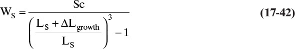
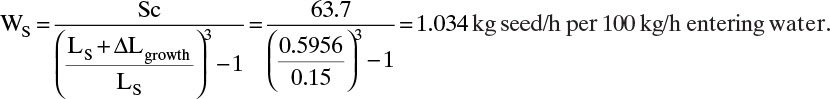
17.8 Batch and Semibatch Crystallization
In a standard batch, cooling crystallization a charge of hot, saturated solution including seed crystals is fed to a tank, the tank is cooled and stirred, and at the end of the batch crystals are harvested. If removal of the solvent by evaporation is required to achieve crystallization, then the operation is inherently semibatch. For a semibatch evaporative crystallizer the tank is heated and exiting vapor is condensed. There is discontinuous addition of feed and removal of crystal product, but solvent removal is continuous. Antisolvent crystallization is also inherently semibatch since antisolvent is typically added during the crystallization. To avoid writing “batch and semibatch” throughout this section, the term batch is used to include both batch and semibatch processes.
Batch crystallization is used when the production rate does not justify use of a continuous crystallizer. Woods (2007) recommends batch crystallization for production rates less than 0.15 kg/s. Batch crystallization is also employed when the same equipment will be employed to produce several different products, when a stirred tank can be used for a batch reaction followed by batch crystallization, and when avoidance of contamination is critical. The last point is somewhat paradoxical since contamination is more likely to occur in a batch operation. However, each batch can be kept separate, and if a batch becomes contaminated, impurities will not be spread to other batches. In pharmaceutical plants where detailed record keeping is required, documentation of batch processes is easier than documentation of continuous processes. Since all reasons for use of batch crystallization often apply in pharmaceutical processing, most crystallization in this industry is batch with seeding.
Crystallization fundamentals are same for steady-state, continuous operation and for batch operation. Both operations have heat and mass transfer, equilibrium, nucleation, and crystal growth, and regularly shaped, relatively large particles are desired for downstream processing. Scale-up is difficult for both processes because of the differences in mixing between small and large vessels (David and Klein, 2001). Batch processing introduces a time factor and a number of process decisions that are not present in a continuous process. For example, do we design a series of small batches that operate for short periods or a relatively large batch operating for a long period? In a cooling crystallizer how do we control cooling rate? Do we add a different solvent during crystallization? There is typically more opportunity to be creative and try novel processing steps in batch operation.
Although batch crystallization can be done without seeding, control of nucleation is difficult. As a result, most batch crystallizers are seeded, and we assume they are seeded. “For those frequent and difficult purification tasks that crystallization from solution does so well, seed early, seed often, and above all, seed always.” (C. B. Rosas, quoted by Tung et al., 2009, p. 112)
17.8.1 Temperature Control for Batch Cooling Crystallizers
Analysis of CSD for seeded batch processes is similar but more complicated than the analysis presented in Section 17.7 for continuous processes. Assume the following:
1. There is no additional nucleation other than seeds.
2. Crystal growth is independent of crystal size.
3. Seeds are tightly classified and can be represented as a single size, LS.
4. Equal growth occurs on all three crystal faces. Alternate derivations can be done for platelets and needles.
5. Mixing is perfect so that temperature and concentration history for all particles is identical.
During the batch temperature and supersaturation vary. Equation (17-40b) remains valid with a slight change in terms:
![]() and
and ![]() are kg seed/kg initial water and kg product/kg initial water. Since linear growth rate G = dL/dt varies as concentration is changed, ΔLgrowth is
are kg seed/kg initial water and kg product/kg initial water. Since linear growth rate G = dL/dt varies as concentration is changed, ΔLgrowth is
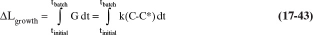
To determine ΔLgrowth we need to specify how cooling (or solvent removal, or the addition of antisolvent) is done so that crystallizer temperature and concentration can be calculated. We also need to determine the effect T and C have on rate constant k and equilibrium concentration C*.
The effects of cooling rates on cooling crystallizers have been extensively studied (Belter et al., 1988; Jones and Mullin, 1974; Jones, 2002; Tung et al., 2009). Assume the crystallizer is well insulated. The amount of heat that needs to be transferred is
The term {Vρfeed/(1 + Cfeed)} is the initial kilograms of water and thus is constant in a cooling crystallizer. The weight of crystals, W(t) kg/(kg initial water), can be obtained from Eq. (17-40a) written for weight W of crystals of size L:
Then, dW/dt is
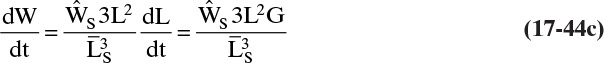
If Cp,magma,V, ρmagma, and ΔHcrystal are constant, Eq. (17-44a) becomes

The easiest operation method is to turn on cooling water at a constant temperature and a constant flow rate. This uncontrolled cooling will initially have a high heat transfer rate, since magma is at its highest temperature and heat transfer surfaces are clean. Heat transfer rate can be determined from one of the forms of the familiar heat transfer equation (Section 11.2), such as
Magma temperature decreases during the batch, and the overall heat transfer coefficient U will not be constant if crystals or precipitates foul the heat transfer surface. As crystallization proceeds and magma cools, the heat transfer rate decreases. Cooling crystallizers are used for systems that have a large negative value of Thus, as temperature drops, drops significantly. Since crystal growth is slow, C drops slowly as the crystals grow. Thus (C – C*) increases significantly unless the cooling rate is controlled and is quite low. A rapid increase in (C – C*) will move the system into the unstable region, as shown in Figure 17-2, and very rapid formation of nuclei is likely (Figure 17-16). These nuclei are added to the seed weight, but nuclei have a much smaller initial length. In this case we return to Eq. (17-38), which becomes
Product 1 is from growth on nuclei, and product 2 is from growth on seeds. The expression is approximate because nuclei are formed at different tinitial values, and ΔLgrowth from Eq. (17-43) will show some spread. However, qualitatively this prediction agrees with experimentally observed bimodal distributions (Tung et al., 2009).
Larger, more uniform crystals are obtained if temperature is controlled. Mullin (2001) and Jones (2002) used the following supersaturation balance:

The first term on the right-hand side is (dT/dt) × (dC*/dT). A series of assumptions need to be made to reduce Eq. (17-47b) to a form that can be integrated analytically to determine temperature as a function of time. Because the system is seeded, we assume there is no nucleation; thus, the last term can be neglected. Additional assumptions to achieve a relatively simple result are that the metastable zone has a constant width, the linear growth rate is size independent, the system is very well mixed, supersaturation is constant, and dC*/dT is constant. The resulting controlled temperature is (Jones, 2002)
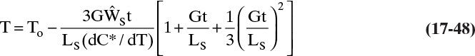
Temperature initially decreases slowly and then at an increasingly rapid rate (see problem 17.D16). This behavior is opposite that of uncontrolled cooling. Experimental results obtained with controlled cooling are compared in Figure 17-22 to results from uncontrolled cooling (Jones and Mullin, 1974). Median crystal size is much larger with controlled cooling.
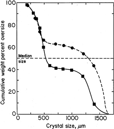
FIGURE 17-22. Experimental CSD for batch crystallization comparing uncontrolled to controlled cooling. ![]() Uncontrolled, • controlled, following Eq. (17-48). Jones, A. G., and J. W. Mullin (1974). “Programmed Cooling Crystallization of Potassium Sulphate Solutions,” Chem. Eng. Sci., 29, 105. Reprinted with permission.
Uncontrolled, • controlled, following Eq. (17-48). Jones, A. G., and J. W. Mullin (1974). “Programmed Cooling Crystallization of Potassium Sulphate Solutions,” Chem. Eng. Sci., 29, 105. Reprinted with permission.
Improved results can often be obtained by adding seeds at several times during the batch (Tung et al., 2009).
17.8.2 Antisolvent Crystallization
Antisolvent crystallization is purposeful addition of a material that reduces solute solubility to induce nucleation and crystal growth. An example is shown in Figure 17-23 where different salts were originally dissolved in water, and methanol was added as an antisolvent (Lozano, 1976). Clearly, methanol is not an effective antisolvent for MgCl2. When an antisolvent is used, it has to be recovered. An additional antisolvent recovery step must be added to Figure 17-1. Antisolvent crystallization is most commonly practiced in the pharmaceutical industry with semibatch crystallizers (Tung et al., 2009).
“Addition of an antisolvent is potentially the best method to achieve controlled and scalable particle size distribution (PSD).” (Tung et al., 2009, p. 179) These authors proceed to clarify that addition of antisolvent must be carefully controlled to increase particle sizes. Addition of all antisolvent at the start of batch crystallization drastically reduces solubility of solute and can easily take the concentration through the metastable zone into the unstable zone shown Figure 17-2. This can lead to the solute “crashing out.” With organic compounds, crashing out may result in oiled-out drops that can harden into gum (not the kind of gum you chew). Cases in which one wants the solute to crash out and precipitate quickly are discussed in Section 17.9.
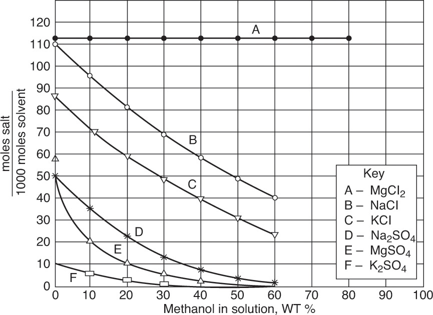
FIGURE 17-23. Effect of methanol on solubility of common salts at 30°C. Abscissa is on a salt-free basis. Lozano, J. A. F., Ind. Engr. Chem. Process Design Develop., 15 (3), 445 (1976). Copyright 1976, American Chemical Society. Reprinted with permission.
Control of CSD is achieved by controlled addition of antisolvent and seeds. One approach that prevents excessive nucleation is to add antisolvent until the mixture is slightly supersaturated, stop addition of antisolvent, and add seeds. The challenge is to do this addition reproducibly batch after batch. If seeds are added too soon, the solution will not be supersaturated, and some or all seeds will dissolve. If seeds are added too late, excessive nucleation may have already occurred. This timing problem is similar to the timing problem for controlling temperature during batch crystallization, and programmed solutions for anti-solvent addition are similar. After seeds have had time to grow and reduce concentration to close to equilibrium, more antisolvent is slowly added.
By definition, seeds are not very soluble in antisolvent. Thus, another approach that can be helpful is to slurry the seeds in antisolvent, and add the slurry as the concentration approaches or just passes saturation. Antisolvent serves as a driving force for crystallization, and seeds provide surface area for growth. Calculations for antisolvent crystallization depend on the solubility reduction caused by the antisolvent. Example 17-15 explores addition of methanol for crystallization of sodium chloride.
EXAMPLE 17-15. Antisolvent crystallization
200 kg of saturated aqueous sodium chloride feed at 30°C is to be crystallized by adding methanol, which is an antisolvent. We add enough methanol to make the weight fraction of methanol in solvent = 0.300 on a salt-free basis.
A. How many kg of methanol do we add?
B. How many kg of anhydrous NaCl crystallize?
Data: MW NaCl = 58.44, MW water = 18.016, MW CH3OH = 32.04
Solution
Preliminary calculations: From Table 17-1 saturation is 36.3 kg NaCl/100 kg water.
Wt% NaCl = 100 × (kg NaCl)/(kg NaCl + kg water)= 100(36.3/136.3) = 26.63. 200 kg solution × 0.2663 = 53.265 kg salt. 200 – 53.265 = 146.735 kg water.
A. Amount of methanol to add: For 30 wt% methanol (salt free): 0.3 = x kg methanol/(146.735 kg water + x). Solve for x = 62.886 kg methanol added.
B. To use Figure 17-23 we need to convert between moles and kilograms.
kmol water = kg water/MW water = 146.735/18.016 = 8.145 kmol.
Initial kmol salt = kg salt/MW salt = 53.265/58.44 = 0.9114. Initial kmol salt / kmol water = 0.9114/8.145 = 0.1119. Initial mole salt/1000 mol water = 111.9, which agrees reasonably well with Figure 17-23 for 0% methanol.
30 wt% methanol, kmol methanol = kg methanol/MWmethanol = 62.886/32.04 = 1.963 kmol.
Total kmol solvent = 8.145 + 1.963 = 10.108 kmol.
From Fig. 17-23 at 30 wt% methanol, ordinate for NaCl = 68.75 or 0.06875 kmol salt /kmol solvent. kmol salt in solution = 0.06875 (10.108 kmol solvent) = 0.6949 kmol NaCl in solution. Moles salt crystallized = initial – final = 0.9114 – 0.6949 = 0.2165 kmol salt = 12.652 kg. Yield = (12.652/53.265) × 100 = 23.8%.
Comments
1. Most of the calculations are required to convert back and forth between the two sets of units used in Figure 17-23.
2. Common salt is recovered from seawater by solar evaporation in ponds, which is a form of evaporative crystallization similar to Example 17-5. We keep using that method instead of switching to methanol as an antisolvent.
17.9 Precipitation
Precipitation has a number of meanings ranging from producing amorphous solids to rapid formation of crystals to formation of rain or snow in meteorology (Jones, 2002). In this section precipitation refers to the rapid formation of solids, which can be amorphous or crystalline. Equipment for precipitation is usually a tank with a mixer. Precipitation is often induced by adding an antisolvent or a salt (salting out). Rapid precipitation often occurs with reverse addition in which the feed is added to the antisolvent or salting-out solution. Crystals produced in reverse addition crystallization are quite small. In pharmaceutical formulations small crystals are sometimes desired as they dissolve faster and deliver the drug faster than large crystals.
17.9.1 Precipitation by Antisolvent Addition
Addition of antisolvent or reverse addition to antisolvent is frequently used for precipitation of moderate molecular weight molecules such as antibiotics and for high molecular weight solutes such as proteins. For moderate molecular weight solutes, the original (effective) solvent is often an organic liquid, and the most common antisolvent is water.
Proteins will be dissolved in water that is buffered, has a moderate ionic strength (0.05 to 0.2 M), and has pH adjusted to pI (pI is the isoelectric point where the net charge on the protein is zero) to minimize protein solubility. The antisolvent is typically an organic such as acetone, ethanol, or polyethylene glycol (PEG). The volume percent of solvent required for precipitation can usually be correlated with an empirical equation (Belter et al., 1988):
For acetone a good fit to the data is obtained with a = 1.8 and b = 0.12. Thus, if we want to precipitate a protein at its pI with a molecular weight of 100,000, the volume percent of acetone needed is
Vol% acetone = 1.8 – 0.12 In (100,000) = 0.418%
Clearly, acetone is effective. If there are other proteins in the feed, they probably have somewhat different PI values. Proteins are more soluble in water when they have a net charge (i.e., not at their PI). Thus, precipitation does some preliminary separation. When precipitating proteins, we need to be concerned about denaturing protein. In the pharmaceutical industry chemical engineers usually work on a team that includes biochemists and industrial pharmacists.
17.9.2 Precipitation by Salting Out
Charged species such as salts and proteins can often be precipitated by adding additional salt (salting out). For low molecular weight salts, the added salt usually has an ion in common with the target salt. For example, if we have AgBr in the solution and add NH4Br, Br– is a common anion. Salts that completely dissociate into anions and cations and have an activity coefficient of unity at saturation have a constant solubility product, KS(T) (Belter et al., 1988; Mullin, 2001). The solubility product for a monovalent salt such as AgBr is
KS,AgBr(T) = [Ag+][Br–]
At 18°C, KS,AgBr = 4.1 × 10⁻¹³ (mol/L)2 (Mullin, 2001). In the literature [ ] refers to concentration in moles/L. If KS,AgBr(T) > [Ag+][Br–], there is no precipitation. If KS,AgBr(T) < [Ag+] [Br–], then there is precipitation until KS,AgBr(T) = [Ag+][Br–].
For a divalent salt such as lead iodide, PbI2, the solubility product is
KS,PbI2 = [Pb+2] [I–]2
In general, if we have a salt, (Cation)m, (Anion)n, or CmAn, that completely dissociates, the solubility product is defined as
If KS,CmAn(T) > [C+m]m[A–n]n, there is no precipitation.
The definition in Eq. (17-50a) assumes that the activity coefficients are all unity. The solubility parameter that is constant at higher concentrations is
As a rule of thumb Eq. (17-50a) is reasonably accurate (γ values are close to 1.0) for concentrations less than about 10–3 mol/L (Mullin, 2001). Since AgBr is not very soluble, concentrations are low, and KS,AgBr is constant.
If we start with a saturated solution of AgBr and add AgNO3 or NH4Br, the concentration [Ag+] or [Br–] increases, respectively. The product of concentrations [Ag+][Br–] > KS,AgBr, and AgBr precipitates until [Ag+][Br–] = KS,AgBr. AgNO3 or NH4Br do not precipitate because they are both more soluble than AgBr. If a large amount of NH4Br is added, [Br–] will be high. To achieve equilibrium with [Ag+][Br–] = KS,AgBr, [Ag+] must become very low, which requires that essentially all silver precipitates as AgBr. Salting out is illustrated in Example 17-16.
EXAMPLE 17-16. Salting out with a common ion
We have 1.0 liter of aqueous solution of PbI2 that is [PbI2] = 0.0012 mol/L.
A. Is this solution saturated at 18°C?
B. If we add 0.002 moles of NH4I, is a precipitate formed? If yes, how much precipitate?
Solution
A. At 18°C concentration solubility product for PbI2, KS,PbI2 = 9.3 × 10⁻⁹ (mol/L)3 (Mullin, 2001). For the concentration [PbI2] = 0.0012 mol/L the solubility product is [Pb+2][I–]2 = [0.0012][2 × 0.0012]2 = 6.91 × 10⁻⁹(mol/L)3, which is less than KS,PbI2= 9.3 × 10⁻⁹(mol/L)3; thus, solution is not saturated.
B. Add 0.002 mol NH4I, which according to Table 17-1 is very soluble. If there is no precipitate, concentration of I becomes [I–] = 0.002 +2 × 0.0012 = 0.0044. Then the solubility product is [Pb][I]2 = [0.002][0.0044]2 = 2.23 × 10⁻⁷, which is greater than KS,PbI2, so there must be precipitation.
For a basis of 1.0 liter of solution, let x = moles PbI2 that precipitate. Then solubility calculation at equilibrium is [0.0012 – x][0.0044 – 2x]2 = 9.3 × 10⁻⁹.
Solving for x with a spreadsheet and Goal Seek, x = 0.000445 moles PbI2 precipitate. Then
[PbI2] = 0.0012 – 0.000445 = 0.000755 mol/L.
Concentration of Pb+2 in the solution is the same, [Pb+2] = 0.000755 mol/L. Concentration of I– is
[I–] = 0.002 + 2 × 0.000755 = 0.00351 mol/L.
In this equation 0.002 is moles of I– added with NH4I, and the second term is from dissociation of 0.000755 mol/L of PbI2 into two moles of I–.
Check. The solubility product is
[Pb][I–]2 = (0.000755)(0.00351)2 = 9.3 × 10⁻⁹ (mol/L)3.
Thus, the solution is at equilibrium.
Salting out is also commonly used to precipitate proteins. Even at their pI, proteins have positively charged amino acids and negatively charged carboxylic acids, although their net charge is zero. The number of charged groups may be quite large. Instead of adding a common ion, which would be an expensive amino acid or carboxylic acid, proteins are salted out by adding large amounts of a common salt. The effectiveness of anions for protein precipitation follows the Hofmeister series (Belter et al., 1988; Rothstein, 1994):
while the cation effectiveness is
Relatively high salt concentrations are required for precipitation of proteins. Since ammonium sulfate is considerably less expensive than ammonium citrate and ammonium phosphate and almost as effective, ammonium sulfate has become the standard choice for protein precipitation. Because there is no common ion and salt concentrations are quite high, Eq. (17-50a) does not apply to protein precipitation. Instead the empirical Cohn equation is used for protein precipitation at high salt concentrations (Belter et al., 1988; Rothstein, 1994).
Empirical constant β depends on the protein but not the salt, and empirical constant K depends on the salt but not the protein. If solubility measurements are available at two salt concentrations, the values of β and K can be determined (see Problem 17.D19).
Ammonium sulfate precipitation also does preliminary separation between proteins with different pI values. Since protein concentrations are typically significantly less than salt concentration, there is often little interaction between different proteins in solution. In this case Eq. (17-52) can be applied to each protein. Each protein will have a different value of β (protein, pH, T), but the value of K (salt) should be essentially identical for all proteins in the solution.
References
Abegg, C. F., J. D. Stevens, and M. A. Larson, “Crystal size distribution in continuous crystallizers when growth rate is size dependent,” AIChE Journal, 14, 118 (1968).
Aqueous Solutions Aps, www.phasediagram.dk/binary/magnesium_sulfate.htm, accessed October 20, 2015.
Beckmann, W., “Basics of Industrial Crystallization from Solution,” in Beckmann, W. (Ed.), Crystallization: Basic Concepts and Industrial Application, Wiley-VCH Verlag GmbH & Co., Weinheim, Germany, 2013.
Belter, P. A., E. L. Cussler, and W.-S. Hu, Bioseparations: Downstream Processing for Biotechnology, Wiley-Interscience, New York, 1988.
Bennett, R. C., and M. Van Buren, “Commercial Urea Crystallization,” Chem. Engr. Prog. Symp. Ser., 65 (95), 44 (1969).
Berglund, K. A., “Analysis and Measurement of Crystallization Utilizing the Population Balance,” in Myerson, A. S. (Ed.), Handbook of Industrial Crystallization, 2nd ed., Butterworth-Heinemann, Woburn, MA, 2002, Chapter 4.
David, R., and J. P. Klein, “Reaction Crystallization,” in Mersmann, A. (Ed.), Crystallization Technology Handbook, 2nd ed., revised and expanded, Marcel Dekker, New York, 2001a, pp. 513–561.
Dean, J. A. (Ed.), Lange’s Handbook of Chemistry, 13th ed., McGraw-Hill, New York, 1985.
Garside, J., and M. B. Shah, “Crystallization Kinetics from MSMPR Crystallizers,” Ind. Eng. Chem. Process Design Develop., 19, 509 (1980).
Genck, W. J., “Crystallization from Solutions,” Section 2.3, in Schweitzer, P. A. (Ed.), Handbook of Separation Techniques for Chemical Engineers, 3rd ed., McGraw-Hill, New York, 1997.
Genck, W. J., “Crystallization from Solution,” in Green, D. W., and R. H. Perry (Eds.), Perry’s Chemical Engineers’ Handbook, 8th ed., McGraw-Hill, New York, 2008, pp. 18-39 to 18-59.
Green, D. W., and R. H. Perry (Eds.), Perry’s Chemical Engineers’ Handbook, 8th ed., McGraw-Hill, New York, 2008.
Jones, A. G., Crystallization Process Systems, Butterworth-Heinemann, Woburn, MA, 2002.
Jones, A. G., and J. W. Mullin, “Programmed Cooling Crystallization of Potassium Sulphate Solutions,” Chem. Eng. Sci., 29, 105 (1974).
Lozano, J. A. F., “Recovery of Potassium Magnesium Sulfate Double Salt from Seawater Bittern,” Ind. Engr. Chem. Process Design Develop., 15, 445 (1976).
McCabe, W. L., “Crystal Growth in Aqueous Solution,” Industrial Engineering Chemistry, 21, 30 (1929).
Mersmann, A. (Ed.), Crystallization Technology Handbook, 2nd ed., revised and expanded, Marcel Dekker, New York, 2001a.
Mersmann, A., “Particle Size Distribution and Population Balance,” in Mersmann, A. (Ed.), Crystallization Technology Handbook, 2nd ed., revised and expanded, Marcel Dekker, New York, 2001b. pp. 145–186.
Mersmann, A., C. Heyer, and A. Eble, “Activated Nucleation,” in Mersmann, A. (Ed.), Crystallization Technology Handbook, 2nd ed., revised and expanded, Marcel Dekker, New York, 2001, pp. 76–80.
Moyers, C. G., Jr., and Rousseau, R. W., “Crystallization Operations,” Chapter 11 in Rousseau, R. W. (Ed.), Handbook of Separation Process Technology, McGraw-Hill, New York, 1987.
Muir, R. F., and C. S. Howat, “Predicting Solid-Liquid Equilibria from Vapor-Liquid Data,” Chemical Engineering, 89 (4), 89 (Feb. 22, 1982).
Mullin, J. W., Crystallization, 4th ed., Butterworth-Heinemann, Woburn, MA, 2001.
Myerson, A. S. (Ed.), Handbook of Industrial Crystallization, 2nd ed., Butterworth-Heinemann, Woburn, MA, 2002.
Myerson, A. S., and R. Ginde, “Crystals, Crystal Growth and Nucleation,” in Myerson, A. S. (Ed.), Handbook of Industrial Crystallization, 2nd ed., Butterworth-Heinemann, Woburn, MA, 2002, pp. 33–66.
National Institute of Standards and Technology (NIST), “Thermophysical Properties of Fluid Systems,” http://webbook.nist.gov/chemistry/fluid. An alternate presentation of the NIST steam table data: https://www.ohio.edu/mechanical/thermo/property_tables/H2O, accessed October 10, 2015.
Perry, R. H., and D. W. Green (Eds.), Perry’s Chemical Engineers’ Handbook, 6th ed., McGraw-Hill, New York, 1984.
Pickering, S. U., J. Chem. Soc. (London), 63, 998 (1893).
Prudich, M. E., “Crystallization from the Melt,” in Green, D. W., and R. H. Perry (Eds.), Perry’s Chemical Engineers’ Handbook, 8th ed., McGraw-Hill, New York, 2008, pp. 20-3 to 20-13.
Randolph, A. D., and M. A. Larson, Theory of Particulate Processes: Analysis and Techniques of Continuous Crystallization, 2nd ed., Academic Press, New York, 1988.
Rothstein, F., “Differential Precipitation of Proteins: Science and Technology,” in R. G. Harrison (Ed.), Protein Purification Process Engineering, New York, Marcel Dekker, 1994, pp. 115–208.
Tung, H.-H., E. L. Paul, M. Midler, and J. A. McCauley, Crystallization of Organic Compounds: An Industrial Perspective, Wiley, New York, 2009.
Walas, S. M., Phase Equilibria in Chemical Engineering, Butterworths, Boston, 1985.
Wankat, P. C., Rate-Controlled Separations, Elsevier (currently published by Springer), 1990.
Wibowo, C., “Solid-Liquid Equilibrium: The Foundation of Crystallization Process Design,” Chem. Engr. Progress, 110 (3), 37 (March 2014).
Witt, W., and T. Allen, “Particle-Size Analysis,” in Green, D. W., and R. H. Perry (Eds.), Perry’s Chemical Engineers’ Handbook, 8th ed., McGraw-Hill, New York, 2008, pp. 21-8 to 21-19.
Woods, D. R., Rules of Thumb in Engineering Practice, Wiley-VCH, Weinheim, Germany, 2007.
A1. Why is it more difficult to reach equilibrium in crystallization than in distillation or extraction?
A2. Why does a sieve analysis tend to size platelets (Figure 15-7D) based on the second-largest dimension? Assume that holes in the sieve are square.
a. Based on the data in Table 17-1, rank the cations (NH4, Ba, Ca, Cu, Mg, Mn, Ni, K, Ag, Na) in order of their solubility in water.
b. Based on the data in Table 17-1, rank the anions (C2H3O2, Br, Cl, F, I, NO3, SO4) in order of their solubility in water.
a. List three compounds from Table 17-1 that would be good candidates for cooling crystallization and explain why.
b. List three compounds from Table 17-1 that would be good candidates for evaporative crystallization and explain why.
A5. Your boss is of the “more is better” school. If a cooling crystallizer works well from 80°C to a cold temperature, she thinks it should be pushed up to 100°C. You think she is sometimes correct and sometimes wrong. From Table 17-1 give an example that shows she is correct and an example where she is wrong.
A6. The text states that for seeded crystallizers, “within limits, supersaturation can be increased to increase growth rate.” What are the limits?
A7. In Example 17-14 part a, ΔLgrowth = 0.2971 mm compared to 0.2918 mm in Example 17-13. Why does the very sharp seed distribution (LS = 0.15 mm for all particles) show more growth than the slightly wider distribution (LS = 0.13, 0.15 and 0.17 mm) despite the same median particle size?
A8. Figure 17-2 shows a metastable region in which a crystallization system can be supersaturated. Does an equivalent region exist for vapor-liquid equilibrium? If yes, why is this region not considered in the design calculations?
B. Generation of Alternatives
B1. Develop a batch or semibatch crystallization for a nonvolatile solute dissolved in water and available, but not saturated, at 65°C. Solubility in water is moderately temperature dependent, and dC*/dT > 0. Solubility is significantly less in organic solvents than in water. The solute is not charged. Outline two or more operating procedures that will give a high yield of relatively large crystals. Give reasons for your choices.
C. Derivations
C1. Derive Eq. (17-4g).
a. Derive Eq. (17-24a) and then Eqs. (17-24b) and (17-24c).
b. Derive Eq. (17-26a) and then Eqs. (17-26b) and (17-27).
c. Derive Eq. (17-29a) and then Eqs. (17-29b) and (17-30).
d. Derive Eq. (17-31).
C3. The text states, “The weighted average crystal length = 3.67 Gτ.” Prove this result is correct.
C4. Equations (17-37) and (17-40a) assume equal growth on all three faces. Derive equations that correspond to Eqs. (17-40a), (17-40b), and (17-14c) if there is equal growth on two faces and very slow growth (approximate as zero growth) on the third face. Assume the two growing faces are the same size in the seed crystals. This growth pattern occurs with platelets.
C5. If birth and death rates are not negligible, show that Eq. (17-21a) for a steady-state crystallizer becomes
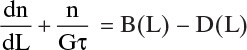
C6. Derive Equation 17-7c.
D. Problems
*Answers to problems with an asterisk are at the back of the book.
D1.* A saturated aqueous solution of CuSO4 at 60°C is cooled in a cooling crystallizer (no loss of water) to 0°C. The product crystals are hydrate CuSO4·5H2O. If we start with 1000 kg of water and add anhydrous CuSO4 until the feed solution is saturated,
a. How many kg of product hydrate are produced?
b. How many kg of water are in the mother liquor?
c. How many kg of anhydrous CuSO4 are in the mother liquor?
D2. 10.0 kg adipic acid is dissolved in 13.1 kg water at 90°C. After filtering to remove material that has not dissolved, the solution is cooled to 35°C. At 35°C crystals form and are removed and dried. During the operation an estimated 10% of the water evaporates.
a. What weight of crystals is recovered?
b. What is the yield?
Data: The solubility of adipic acid at 90°C = 80 kg/100 kg water and at 35°C = 5 kg/100 kg water (Belter et al., 1988). The stable form is anhydrous.
D3. 1000 kg/h of an aqueous feed that is 20 wt% Na2CO3 at 80°C is fed to a vacuum crystallizer operating at 0°C. To concentrate feed and control the crystal product, 350 kg/h of vapor are boiled off. Data are in Figure 17-12, and partial pressure of aqueous Na2CO3 at 0°C is in Green and Perry (2008, Table 2-27).
a. What are the compositions of magma, crystals, and mother liquor?
b. What is crystallizer pressure?
c. What are the flow rates of magma, A, Sc, and L?
d.* How much energy needs to be removed or added in kJ/h?
D4. Since sodium sulfate has reverse solubility, an evaporative crystallizer operating at 100°C is used to concentrate and crystallize 1500 kg/h of an aqueous feed at 100°C that contains 28.57 wt% sodium sulfate.
a. How much vapor needs to be removed (kg/h) to saturate the feed?
b. After step a, we remove an additional 550 kg/h of vapor. How many kg/h of anhydrous crystals are obtained?
c. What is FW,out?
D5. A mixture of β-methylnaphthalene + β-chloronaphthalene (βcn) at 1.0 atm (Figure 17-8a) has liquid and solid in equilibrium at 50°C.
a. What are the mole fractions (x![]() cn) of the liquid and solid phases in equilibrium?
cn) of the liquid and solid phases in equilibrium?
b. What ranges of initial mole fraction can produce an equilibrium mixture at 50°C?
c. If the initial value of x![]() cn = 0.5 and the liquid and solid are in equilibrium at 50°C, what fraction of the original feed is liquid?
cn = 0.5 and the liquid and solid are in equilibrium at 50°C, what fraction of the original feed is liquid?
d. If the liquid in parts a and c is removed and then cooled to 45°C, what are the mole fractions of the liquid and solid in equilibrium?
e. If the liquid in parts a and c is removed and then cooled to 35°C, what is the average mole fraction of the solid?
D6.* 1000 g of water at 30°C contains 300 g KCl (not saturated). Methanol (CH4O) is added to make a 40 wt% methanol (salt-free basis) solution of solvents. KCl does not form a hydrate. Data are in Figure 17-23.
a. How many grams of methanol are added?
b. How many grams of KCl crystallize?
D7. In crystallization of potassium chloride with a 100°C feed and the crystallizer operating at 20°C, we obtain G = 4.0 × 10⁻⁷ m/s. The crystallizer’s volume is 0.2 m3, and the feed rate is 1000 kg/h. When operated without seeds, the crystals produced are too small. Your boss decides to seed and use a new crystallizer with volume = 1.0 m3 but with the same throughput of feed and the same supersaturation, C – C*, as the current crystallizer. Desired crystal size is 2.56 mm. If the seed crystals are available with a very tight size distribution, what size of seed crystals, LS (mm), and what weight of seed crystals (kg/h) should be used?
Data: ρf = 1209 kg/m3, KCl does not form a hydrate. Crystals are cubic in shape with equal growth on all faces, and kv = 1.0. Note: Watch your units!
D8. Urea crystallization (kv = 1.0, τ = 5.9 h, ρc = 1.33 g/cm3) resulted in the following partial sieve analysis (screen numbers in the second row are weight % of the total amount of crystals collected on this screen). MT,exp = 510 g/L. Although the data for the other weight % of total weight values were lost in a computer crash, estimate G in m/s with the available data.
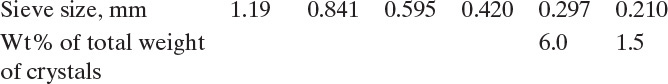
D9. A saturated feed of potassium chloride at 100°C is fed to a cooling crystallizer operating at 20°C. We obtain G = 4.0 × 10⁻⁷ m/s. Crystallizer volume is 0.2 m3, and the feed rate is 1000 kg/h. We screen 1.0 L of magma and collect crystals between sieves with sizes of 0.500 mm and 0.354 mm. Data: ρf = 1209 kg/m3, KCl does not form a hydrate.
a. What weight of crystals is collected between these two sieves?
b. What is the median size of mass distribution?
D10.* Discard the data point for the size 14 screen in Example 17-9, and find G and no.
* The solution is given in Example 17-9.
D11. Repeat Example 17-10 but discard the data point for the size 14 screen. Find G and no.
a.* Predict the complete screen analysis for Example 17-11. The stack of screens used the following Tyler mesh screens: 10, 12, 14, 20, 24, 32, 42, 60, 80.
* The solution for size 24 to 20 screens is given in Example 17-11.
b. How many grams of undersized crystals are not collected?
D13. Example 17-14 Part B illustrates a method to increase the size of product crystals by seeding. An alternate procedure that might be feasible in some situations is to keep supersaturation, V, Qout, and ΔLgrowth constant and increase the size of the seeds, LS, to obtain desired product size, Lp. Repeat Example 17-14 Part B to obtain a particle size of Lp = 0.60105 mm with constant supersaturation, τ, and ΔLgrowth but with larger seeds. Find new values of LS and of WS.
D14.* A 3.2-m3 cooling crystallizer is seeded with 10.0 kg/h of seeds that have a mean size of 0.006 mm. We want to increase the size of product crystals from the current 0.024 mm to 0.056 mm. Crystals are cubic and have equal growth on all faces. Inlet and outlet temperatures of the crystallizer, outlet volumetric flow rate, supersaturation, and size distribution of seeds are constant. What seeding rate (kg/h) and volume (m3) of crystallizer will produce product crystals of the desired size?
D15. A 3.0-m3 cooling crystallizer is operating over a temperature range that gives Cin = 82 kg solute/100 kg water and Cout = 35 kg solute/100 kg water. FW, in = 266 kg water/h. No hydrates are formed. Density of concentrated feed = 1200 kg/m3. Currently we are adding 2.97 kg/h of seed crystals with an average size of LS = 0.021 mm to the feed and producing product crystals that are too small. Increase product crystals to Lp = 0.24 mm. Keep magma density MT, weight of product crystals Wp, and outlet volumetric flow rate Qout constant.
a. What are the current values of Qout m3/h, MT kg/m3, Wp kg/h, ΔLgrowth mm, and product crystal size Lp mm?
b. What size crystallizer and what weight of seeds kg/h are required to produce crystals of the desired size?
D16. We want to use controlled cooling of a batch crystallizer that is crystallizing KCl from an aqueous solution. The feed is saturated at the initial temperature of 90°C, and the final temperature is 20°C. G = 7.16 × 10⁻⁵ mm/s, seed size Ls = 0.14 mm, liquid volume in the tank = 1 m3, WS = 2 kg seeds/100 kg initial water, and densities can be estimated from the following density data for aqueous KCl solutions (Green and Perry, 2008, Table 2-76):
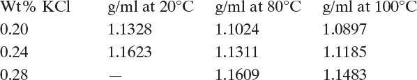
a. Find kg of water and the total weight of the seeds used.
b. Plot the cooling curve (temperature versus time) from Eq. (17-48) for controlled cooling.
c. Find the total batch time.
a. At 18°C the concentration solubility product of AgBr is KSAgBr = 4.1 × 10⁻¹³ (mol/L)2 (Mullin, 2001). What is the concentration of AgBr at saturation?
b. If we add 5.0 × 10⁻⁷ mol/L of NH4Br, what is the final solution concentration of AgBr? What fraction of Ag+ precipitates?
c. How many moles/L of NH4Br need to be added to a saturated solution of AgBr at 18°C to precipitate 99% of the silver?
D18.* The concentration solubility product of Al(OH)3 is 1.1 × 10⁻¹⁵ (mol/L)4 (Mullin, 2001). At saturation, what is the concentration of Al(OH)3? Note: This requires some thought. How much of each ion is there in the solution?
D19. At 18°C the concentration solubility product for PbI2 = 9.3 × 10⁻⁹ (mol/L)3 (Mullin, 2001). At saturation what is the concentration of PbI2?
D20. 1000 g of water at 30°C is saturated with K2SO4 (11.0 mol/1000 mol solvent). Methanol (CH4O) is added to make a 40 wt% methanol (salt-free basis) solution of solvents.
a. How many grams of methanol are added?
b. How many grams of K2SO4 crystallize?
K2 SO4 does not form hydrates from this solution. Data are in Figure 17-23.
D21. The solubility of an albumin is approximately 12 g/L at [(NH4)2SO4] = 2.5 M and 0.006 g/L at [(NH4)2SO4} = 3.5 M.
a. Predict albumin solubility at [(NH4)2SO4] = 3.0 M.
b. Predict albumin solubility at [(NH4)2SO4] = 3.75 M.
c. Predict albumin solubility at [(NH4)2SO4] = 2.4 M.
d. Predict albumin solubility at [(NH4)2SO4] = 2.0 M.
e. Which of these predictions is most likely reliable, and which is most likely seriously in error? Explain why.
D22. An aqueous mixture that is 30 wt% Mn(NO3)2, initially at 20°C, is cooled slowly so that it is always at equilibrium. Data are in Figure 17-7.
a. At 0°C what phase(s) are present, and what is (are) their composition(s)?
b. At –20°C what phase(s) are present, and what is (are) their composition(s)?
c. At –20°C how many kg per kg of feed do we have of each phase present?
D23. A saturated sodium nitrate, NaNO3, solution at 100°C at a feed rate of 1000 kg/h of water is sent to a steady-state evaporative crystallizer also operating at 100°C. The evaporative crystallizer evaporates 300 kg/h of pure water vapor. The mixture of the liquid and crystals from the evaporative crystallizer is cooled to 35°C and sent to a steady-state cooling crystallizer also operating at 35°C. Data are in Table 2.1.
a. How many kg of water, how many kg of crystals, and how many kg of dissolved NaNO3 are in the product from the evaporative crystallizer?
b. How many kg of water, how many kg of crystals, and how many kg of dissolved NaNO3 are in the product from the cooling crystallizer?
D24. We mix 1000 kg/h of water at 80°C with 540 kg/h of copper sulphate hydrate crystals. This mixture is cooled to 20°C while evaporating 108 kg/h of water under a vacuum.
a. How many kg/h of hydrated crystals are collected?
b. What mass, kg/h, of anhydrous crystals are collected?
Data: Solubility data are in Table 17-1. MW: Cu = 63.5, S = 32.1, O = 16, H = 1.
D25. We start with 100 kg of water and add 30 kg KCl. We then add 42.86 kg of methanol to the solution. How many kg KCl precipitate? Operation is at 30°C. Data are in Figure 17-23.
D26. We feed 150 kg of water containing 200 kg KCl/(100 kg water) at 99°C to a cooling crystallizer. The crystallizer operates at 37°C.
a. How many kg/h KCl crystals are collected?
b. What is the yield of KCl?
c. We want to increase yield to 85% but cannot cool to a lower temperature. Instead we will evaporate some water and operate the crystallizer at 37°C. How many kg/h should we evaporate?
Data: Table 17-1.
D27. We want to make a solution of citric acid, C3H4OH(COOH)3, which has 200 g of anhydrous citric acid per 100 g of water (according to the data in Table 17-1, 40°C and higher have saturation concentrations higher than this). If we want 10.0 kg of the total solution, how much citric acid hydrate and how much water should we add?
E1. Start with 1000 g water, and dissolve NaCl until it is saturated at 30°C.
a. How many moles of NaCl are in the solution?
b. Now add methanol. How many moles of methanol need to be added to precipitate exactly one-fourth of the moles of NaCl dissolved in part a? Data are in Figure 17-23.
c. Is it possible to precipitate one-half of the moles of NaCl dissolved in part a by adding methanol? Explain your answer.
F. Problems Requiring Other Resources
F1. Find a water-NaCl phase diagram on the Internet.
a. Compare the diagram to others on the Internet to be sure you have a scientifically accurate diagram and not one that is approximate.
b. At 15.0 wt% NaCl what is the freezing temperature, and what crystals are formed?
c. If you start with pure water ice at –5°C, what wt% NaCl is needed to melt the ice? If you keep adding NaCl (T constant at –5°C), at what NaCl weight fraction does it freeze again? What are the crystals?
F2. We have 15.0 kmol of a mixture that is 60 mol% naphthalene and 40 mol% phenol at 100°C. Note: Read the diagram as accurately as you can.
a. When it is slowly cooled, at what temperature do crystals first appear?
b. If the mixture is cooled to 40°C, what are the compositions of liquid product and of crystals?
c. If the mixture is cooled to 40°C, how many kmol of crystals are produced?
Data are available in Walas (1985) and reprinted in Wankat (1990). Use observed data, not calculated curves.
F3. 100 kmol/h of an 8 mol% naphthalene-92 mol% phenol mixture at 40°C is fed to a continuous crystallizer. The crystallizer operates at 33°C. Data sources are in Problem 17.F2.
a. What is the purity of crystals?
b. What is the approximate concentration of the final mother liquor?
c. How many kmol/h of crystals are harvested, and what is the flow rate, kmol/h, of the mother liquor?
F4. Sufficient lactose is dissolved in 5000 g water/min at 80°C to make a saturated solution. This feed is sent to a cooling crystallizer where it is cooled to 10°C.
a. How many g/min of lactose were originally dissolved?
b. How many g/min of crystals precipitate?
H. Spreadsheet Problems
H1.* A cooling crystallizer is crystallizing potassium chloride, KCl, from an aqueous solution at 32°C and p = 1.013 bar. Feed to the crystallizer is initially saturated at 100°C and is cooled to 32°C. The crystallizer holds 2.5 m3 of magma. Total feed rate is 2000 kg/h. Mullin (2001) reports KCl growth is size independent. Assume the crystallizer can be modeled as an MSMPR crystallizer.
Data: Garside and Shah (1980) report population density at 32°C is given by Eq. (17-34).
Density of solutions: See Table 2-76 (Perry and Green, 2008). ρc = 1998 kg/m3, kv = 1.0. Crystal form, anhydrous. KCl solubilities: Table 17-1.
a.* Find G (m/s) and weight-average crystal length = 3.67 Gτ.
b. If we desire a weight-average crystal length = 3.67 Gτ = 1.70 mm, what volume of crystallizer is required?
Chapter 17 Appendix. Spreadsheets
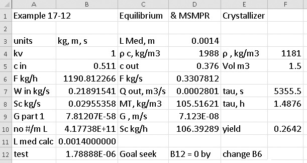
FIGURE 17-A1. Spreadsheet for Example 17-12. Test = 1,000,000 * (B11 – D3).
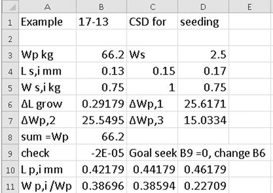
FIGURE 17-A2. Spreadsheet for Example 17-13. Check = 1000 * (B8 – B3).